
Virtual Diagnostic Suite for Electron Beam Prediction and Control at FACET-II
by
 , ,
, ,
Claudio Emma
1,*,† ,
,
Auralee Edelen
1,†,
Adi Hanuka
1,†,
Brendan O’Shea
1,† and
Alexander Scheinker
2,† 1
SLAC National Accelerator Laboratory, Menlo Park, CA 94025, USA
2
Los Alamos National Laboratory, Los Alamos, NM 87545, USA
*
Author to whom correspondence should be addressed.
†
These authors contributed equally to this work.
Information 2021, 12(2), 61; https://doi.org/10.3390/info12020061
Submission received: 1 January 2021
/
Revised: 25 January 2021
/
Accepted: 27 January 2021
/
Published: 31 January 2021
(This article belongs to the Special Issue Machine Learning and Accelerator Technology)
Abstract
:We discuss the implementation of a suite of virtual diagnostics at the FACET-II facility currently under commissioning at SLAC National Accelerator Laboratory. The diagnostics will be used for the prediction of the longitudinal phase space along the linac, spectral reconstruction of the bunch profile, and non-destructive inference of transverse beam quality (emittance) while using edge radiation at the injector dogleg and bunch compressor locations. These measurements will be folded into adaptive feedbacks and Machine Learning (ML)-based reinforcement learning controls to improve the stability and optimize the performance of the machine for different experimental configurations. In this paper we describe each of these diagnostics with expected measurement results that are based on simulation data and discuss progress towards implementation in regular operations.
1. Introduction
Experiments at the forefront of e-beam accelerator R&D require increasingly finer measurement and control of the beam properties during acceleration, transport, and delivery to users. For example, research planned at the Facility for Advanced Accelerator Experimental Tests II (FACET-II) [1] under commissioning at the SLAC National Accelerator Laboratory aims to demonstrate an ultra-high gradient Plasma Wakefield Accelerator (PWFA) with the preservation of beam quality as well as study the physics of extreme beams with ultra-short bunch lengths (sub m) and ultra-high peak currents (>100 kA). These kinds of applications pose a challenge for state-of-the-art diagnostics, as the high intensity and very short pulse duration limit the applicability, effectiveness, and accuracy of traditional measurement techniques. This requires a re-thinking of the existing suite of diagnostics that will be used in order to characterize and control the e-beam properties and facilitate the success of the experimental program.
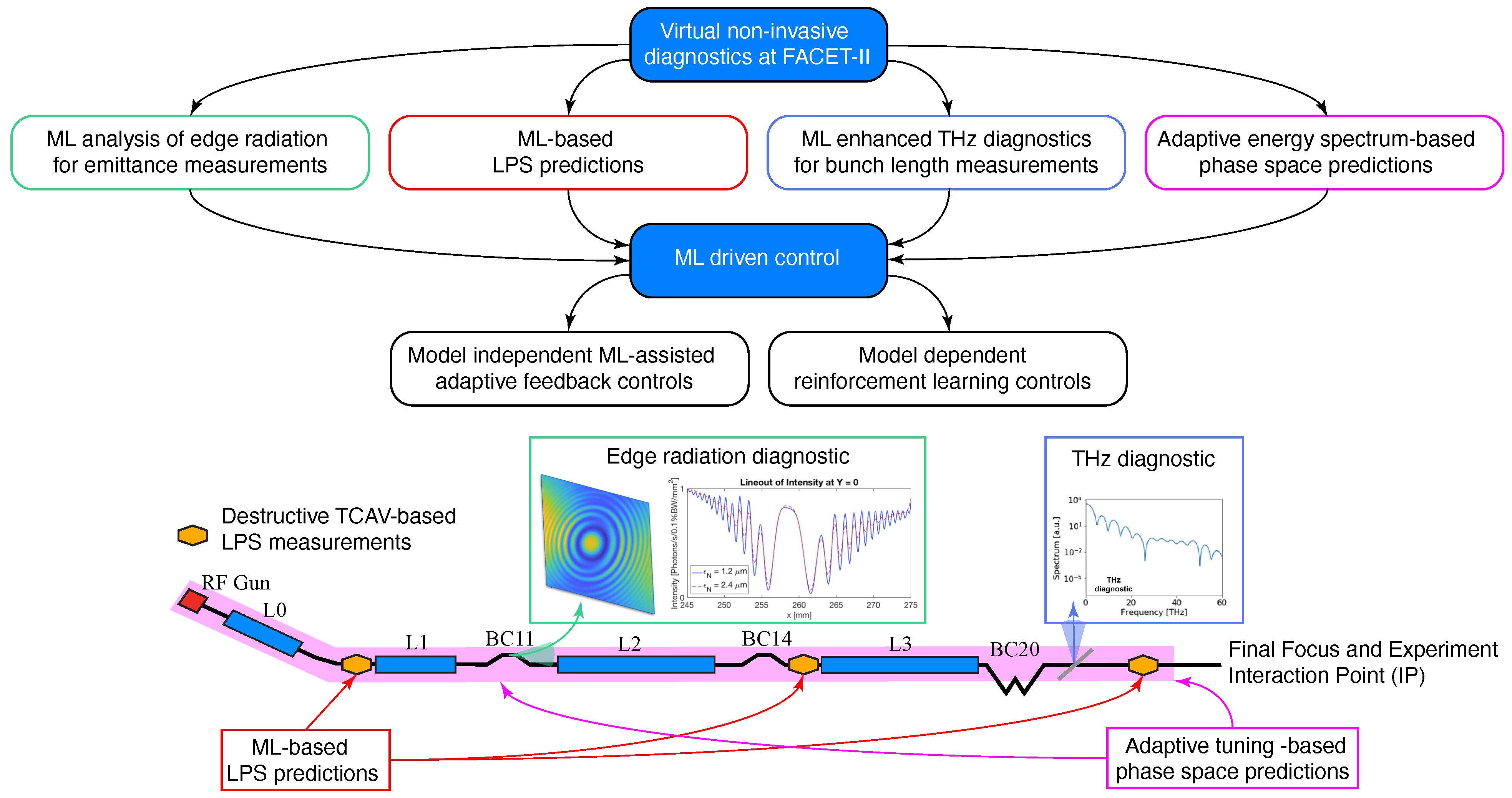
In this paper, we discuss the application of Machine Learning (ML) methods for developing a suite of virtual diagnostics to be used for electron beam prediction and control at the FACET-II facility. These virtual diagnostics will provide a shot-to-shot non-destructive measurement of the electron beam longitudinal and transverse properties along the accelerator and they serve as input for conventional feedbacks and optimization algorithms that are based on reinforcement learning that can tailor the beam properties for specific experimental applications (see Figure 1 for schematic). These diagnostics will work in tandem with traditional measurement techniques to provide otherwise unavailable information to experimenters, which will aid in the machine setup as well as optimization and interpretation of experimental results during offline data analysis. We will discuss a number of examples of ML-applications of FACET-II in this work: the reconstruction of e-beam Longitudinal Phase Space (LPS) along the accelerator, spectral virtual diagnostics for enhancing the accuracy and confidence of beam profile and LPS predictions, ML-based image analysis for inferring e-beam emittance using edge radiation, adaptive model-based 6D phase space predictions, and reinforcement learning controls. We describe the ML methods that are applied in this work in the following section and summarize the key results of each ML-driven diagnostic and control method in Section 3.1, Section 3.2, Section 3.3, Section 3.4 and Section 3.5.
2. Materials and Methods
One of the main running configurations for PWFA experiments at FACET-II will involve accelerating two bunches from the photocathode to the interaction point (IP) at the plasma entrance with specific longitudinal profile properties and drive-witness bunch separation. For a full description of PWFA experiments at FACET-II, see Ref. [2]. A schematic of the FACET-II linac in Figure 1 shows the main components of the accelerator, three linac sections L0–L3 separated by a dog-leg between L0 and L1, two bunch compressors BC11 and BC14, and a final bunch compressor BC20 before the experimental area IP. The major goals for these PWFA experiments will be to demonstrate pump depletion of the 10 GeV drive beam and acceleration of the witness beam to approximately 18 GeV while preserving good beam quality. The nominal beam parameters for the two-bunch pump depletion experiment are a 10 GeV energy, and a few m level normalized transverse emittance, a 150 m bunch spacing, a 2:1 ratio between the peak currents, and a 3:1 ratio in the bunch charge between the drive and witness beam at the entrance of the plasma. The figures of merit for the beam quality will be the preservation of energy spread and emittance of the witness bunch, and these will need to be measured on a shot-to-shot basis for both the incoming distribution and accelerated witness beam. To this end, accurate measurements of the bunch profile entering the plasma are essential in the success of the experimental campaign. Using ML based virtual diagnostics to non-destructively predict the LPS distribution at the entrance of the plasma will provide previously unavailable information that can be used to both understand experimental results from PWFA and tune the beam parameters in order to facilitate the PWFA interaction.
2.1. ML-Enhanced Diagnostics
Previous work has demonstrated the feasibility of using ML models as virtual diagnostics to non-destructively predict the LPS distribution of FACET-II single bunch operation (in simulation) and at LCLS (in experiment) [3]. These studies used neural networks to create a mapping between non-destructive diagnostic inputs (e.g., linac and e-beam diagnostics that are available on a single shot basis) and destructive diagnostic output that measures the beam LPS. What was previously not included in the simulation study of Ref. [3] is the impact of LPS measurement resolution on the ML-based LPS reconstruction. At FACET-II, the LPS distribution of the electron bunch can be destructively measured at the entrance of the plasma with an X-band Transverse Deflecting Cavity (TCAV). The TCAV imparts a transverse kick on the electron beam proportional in strength to an individual electon’s longitudinal position within the bunch. This transverse kick results in a transverse offset downstream and maps the longitudinal profile of the beam to the transverse profile that can be viewed on a downstream screen. The position of the downstream screen is selected, such that there is dispersion in the plane orthogonal to the TCAV kick, thereby simultaneously mapping the electron beam longitudinal and energy profiles (2D LPS) to the horizontal and vertical planes in a single shot. The TCAV operates at a peak voltage of 20 MV and it has a longitudinal resolution of a few m RMS. This introduces a challenge for accurately characterizing the longitudinal bunch profile, as the accelerator is expected to produce very short bunches ( ≤ 1 m) beyond the TCAV resolution. In Section 3.1 of this work, we examine the effect of the TCAV measurement on the performance of the ML-based virtual diagnostic and discuss its application in the FACET-II two-bunch operation mode. We present the results from 3125 Lucretia simulations of the FACET-II linac tracking macro-particles from the exit of the injector (end of L0 before the first dog-leg) to the end of the linac with induced jitter of key accelerator and beam parameters that are described in Table 1. Lucretia [4] is a Matlab-based physics toolbox for modeling single-pass electron linacs and it has been benchmarked against well established codes, such as BMAD [5] and ELEGANT [6]. It includes standard particle tracking features that are employed by established codes, as well as collective effects, including wakefields, longitudinal space charge, and coherent and incoherent synchrotron radiation. The simulation results described in the text start from the end of L0 before the first dog-leg and end at the experimental area IP. The section from the RF gun to L0 is simulated while using the particle tracking code GPT [7]. The simulation data are used to train a ML-based virtual diagnostic for the two-bunch LPS and results show very good agreement between the simulated LPS distribution, as measured by the TCAV and the LPS distribution predicted by the ML model. Because to TCAV resolution limits, there is some discrepancy when we use the projection of the measured LPS distribution to infer the current profile at the entrance of the plasma. This discrepancy affects the accuracy of the ML-based virtual diagnostic for high current shots with short bunch length. We discuss the incorporation of spectral signals in a spectral virtual diagnostic in Section 3.2 in order to flag these shots and increase the confidence and accuracy of the virtual diagnostic predictions.
In addition to longitudinal diagnostics, the transverse diagnostics of the beam emittance are of critical importance for FACET-II’s aim of achieving acceleration in PWFA while preserving beam quality. In order to address this need, we will be implementing a series of single-shot non-destructive emittance measurement based on the interference of edge radiation at the location of bunch compressors (BC11, BC14 and BC20) as well as at the exit of the photoinjector before the first linac section (see Figure 1). These diagnostics will provide a snapshot of the emittance at each point along the linac, allowing for experimenters to outline critical sources of emittance growth. This improves understanding of the beam dynamics in the transport, acceleration, and compression from the photoinjector to the experimental area. The diagnostics will require advanced image analysis in order to obtain a real-time estimate of the beam emittance from the edge radiation interference pattern. This analysis will be conducted using Convolutional Neural Networks (CNNs) that were trained on image data from simulations of the edge radiation inteference pattern with beams of different emittance at different points along the linac. Section 3.3 provides an example of this kind of simulation. We will incorporate signals from the ML-enhanced suite of diagnostics into control methods to improve the quality and stability of the electron beams, as described in the following paragraphs.
2.2. ML-Enhanced Control
While powerful ML methods are able to learn complex input-output relationships in large many parameter systems directly from data, their accuracy will degrade if the system for which they have been trained changes with time. One way to compensate for time variation is to repeatedly re-train several layers of an ML tool, such as a CNN, but this may be problematic for particle accelerator applications, such as FACET-II, where, for example, acquiring new LPS training data requires re-tuning a beam line in order to transport the beam to a TCAV-based diagnostic, rather than to the interaction point. Another approach to dealing with time-varying systems is the use of adaptiive ML that combines model-independent adaptive feedback with data-based ML approaches. Adaptive feedback is, by design, applicable to unknown and changing systems, and it can utilize global approximations that are provided by ML as starting points for tuning. Recently, a first of its kind adaptive ML approach was demonstrated for the automatic control of the LPS of the electron beam in the LCLS FEL [9]. In [9], a neural network was trained to directly map TCAV-based LPS measurements to the accelerator parameters that are required for those beam properties, the NN’s predictions were able to find the correct neighborhood of parameter space, after which extremum seeking was able to adaptively tune all of the parameters to zoom in on and track their optimal settings despite noise and time-variation of both the beam and accelerator parameters.
Adaptive model-independent feedback is a general approach that we aim to utilize together with diagnostics in order to perform active control of the FACET-II beam. Recently, an adaptive tuning method, known as extremum seeking, has been developed for the optimization and stablization of unknown, time-varying, nonlinear dynamic systems that is able to tune many parameters simultaneously based only on noisy measurement data [10]. This extremum seeking method has been implemented for various particle accelerator applications, including virtual diagnostics and beam optimization. In [11], an adaptive extremum seeking feedback-based virtual LPS diagnostic was developed that was able to non-invasively predict TCAV LPS measurements and track changing beam parameters over a wide range of bunch lengths and bunch-to-bunch separation at FACET. Extremum seeking was also recently demonstrated for online multi-objective optimization for simultaneous trajectory control and transverse emittance growth minimization at the electron beam line of the AWAKE plasma wakefield accelerator at CERN by adaptively simultaneously tuning 15 parameters: two solenoids, three quadrupole magnets, and 10 steering magnets [12]. One possible limitation of adaptive feedback is that it is usually based on local iterative methods whose convergence speed may decrease as the number of tuned parameters grows or as the starting conditions of the tuned parameters move further away from the optimum in a high dimensional space. It is impossible to quantify the length of this convergence in general. As with all algorithms (including ML hyperparameters), the convergence time depends on how many parameters are being tuned, on the detailed shape of the high dimensional cost function being minimized or maximized, on how far away from the optimal the initial parameter settings start, and on the hyperparameters of the adaptive tuning scheme. For example, in [12], 10 parameters were routinely tuned within 30 steps, while, in [13], 100 steps were required for six parameters. Extremum seeking has also recently been applied to a form of adaptive reinforcement learning, which is an outgrowth of Optimal Feedback control. Reinforcement learning has recently grown in popularity with the use of ML methods being utilized to learn models for Dynamic Programming problems in order to satisfy the Bellman optimality condition [14]. In [15], a reinforcement learning approach is utilized in which optimal feedback control laws (or “agent policies”) are learned online directly from system data for unknown and time-varying systems. This approach was studied for the optimal control of radio frequency accelerating cavities with characteristics that drift with time, such as cable length changes, resonance frequencies, and analog component fluctuations, due to temperature variations. The use of such adaptive reinforcement learning approach will also be studied for the adaptive diagnostics and controls being designed for FACET-II. Reinforcement learning for various accelerator applications is described in more detail below.
Reinforcement learning approaches can combine both model learning and feedback control. In reinforcement learning an “agent” (i.e., the controller) learns how to interact with an environment over time in order to achieve the highest long-term reward. In the context of accelerator tuning, the “environment” is the accelerator and the reward could be, for example, specific beam shapes one wants to achieve. Critically, reinforcement learning takes the present system state (e.g., system control settings and observable outputs) into account when choosing the next action to take. Over the course of many interactions with the environment, the reinforcement learning algorithm learns to improve its overall control strategy while retaining information regarding previously-visited environmental states. Some reinforcement learning algorithms directly learn a map from system states to actions (a learned policy). Others use a learned model that estimates the likely future reward that will be obtained when specific actions are taken in various observed system states. These predictions can then be combined with simple policies to determine the actions to take. Reinforcement learning has been applied to the problem FEL tuning at LCLS [16] and FERMI@Elettra [17], and it is, at present, being developed for a variety of other online optimization and control tasks in accelerators (for example, round-to-flat beam transforms at UCLA [18], beam size control at AWAKE).
Deep reinforcement learning, which leverages neural networks, is appealing for the task of LPS tuning, in part, because it can directly learn policies from images. Deep reinforcement learning has been used for end-to-end visuomotor control tasks in robotics cite and game-playing tasks where the state of the system is given as an image. In the case of FACET-II, both LPS image and upstream diagnostics, such as the virtual cathode camera (VCC), could be used to inform the present system state. By directly using images, features that otherwise would not be captured by bulk scalar metrics that are derived from the images may be learned from and exploited in tuning, potentially leading to finer control over the LPS. In Section 3.4, we discuss the use of combined adaptive feedback and ML for virtual sic-dimensional (6D) diagnostics of the FACET-II beam’s phase space and for active feedback control of the beam properties.
3. Results
3.1. Longitudinal Phase Space Reconstruction
We present three examples of the simulated LPS profiles at the FACET-II experimental area, as measured by the TCAV shown in Figure 2 with corresponding current profiles and prediction from the ML-based virtual diagnostic. This ML tool is a neural network that takes scalar inputs from accelerator and electron beam diagnostics and outputs a prediction of the 2D LPS image. The diagnostic inputs consist of linac settings (amplitude and phase of RF in the L1 and L2 linac sections) as well as non-destructive measurements of beam properties (peak current and beam centroid at the bunch compressor locations). The diagnostic inputs can be measured non-destructively on a single shot basis and include random offsets to the readings to simulate expected measurement accuracy (see Table 1). The three distributions that are shown represent an under-compressed, over-compressed, and nearly fully-compressed (nominal) beam, respectively. Note that the head of the bunch is on the left of the images. The ML model that we used was a three-layer fully-connected neural network with (500,200,100) neurons in each successive hidden layer and a rectified linear unit activation function for each neuron. The network was trained while using the open source ML library Tensorflow, and two separate models with the same architecture were trained for the 2D LPS prediction and 1d current profile prediction. We see very good agreement between the LPS profiles measured by the TCAV and those predicted by the ML model, as evidenced in Figure 2. There is also good agreement between the ML-predicted current profiles and those that were extracted from the TCAV image. The variety of LPS images input to the ML model for training result from the expected shot-to-shot-jitter of linac and e-beam parameters outlined in the FACET-II Technical Design Report (TDR, see Table 1) [8]. The nominal settings produce a ∼150 m bunch spacing, a 2:1 ratio between the peak currents, and a 3:1 ratio in the bunch charge between the drive and witness beam. The variation in bunch profile from shot-to-shot jitter results in a 9% RMS variation in the drive-witness charge ratio, a 30 m RMS variation in the bunch separation, and a 36% RMS variation in the ratio of the peak current from the nominal settings. These parameter variations are well predicted by the ML model.
The FACET-II two-bunch configuration operates at near full compression and it will generate very short bunches with RMS sizes of a few m putting them at the limit of the TCAV resolution, as discussed above. This means that the values measured for the peak current on the TCAV sometimes differ from the values at the IP and, therefore, so will the prediction from the ML model, which is trained while using TCAV measurements as inputs. We examine this discrepancy in detail in Figure 3, where we show the same current profiles from the three example shots presented in Figure 2 measured on the TCAV and compare this with the current profile that we calculate from the distribution at the IP binned at 0.25 m per pixel. There are a few observations that we can make by looking at Figure 3a–c. The first is that the peak current values that were measured by the TCAV underestimate the true value for shots with peak current greater than ∼35 kA. We note that these high peak currents are greater than those that we plan to deliver for the two-bunch pump depletion experiments outlined in Ref. [2]. Nonetheless, close to the nominal settings (as shown in Figure 3c), the correct value of the ratio of the peak currents may be under-estimated if the witness bunch current profile is poorly resolved by the TCAV measurement. In order to quantitatively understand the limits imposed by the TCAV measurement, we can estimate the longitudinal resolution, as follows:
where is the electron beam energy is the TCAV voltage and wavenumber, is the phase advance between the TCAV and the measurement screen, is the resolution of the screen (we assume 4 m for a transition radiation target), is the beta function at the screen, is the beam emittance, and is the beta function at the TCAV. The ∼35 kA max resolvable peak current come from the constrained optimization of the beta function at the screen and at the TCAV while meeting the beam stay-clear constraints in the experimental area and mitigating the loss of resolution from chromatic errors and emittance growth in the transport. For a 10 m normalized emittance at 10 GeV with a phase advance of 3/2 between TCAV and screen, the optimized values of and are 107 and 6.5 m, giving a resolution of = 4.58 m (see Equation (1)). Given a Gaussian drive bunch at 1.5 nC charge, this corresponds to kA, which is in reasonable agreement with the trend that is shown in the scatter plot presented in Figure 3d.
For shots that are not beyond the TCAV resolution, we can see, from Figure 3d,e, that we can correlate the TCAV measured peak current with the peak current at the IP. These shots are mostly in the region that is defined by kA and kA, as measured on the TCAV. Some shots in this region still show large discrepancy between the TCAV current profile and that measured at the IP, and these represent the spiky ‘double-horn’ type distributions in the drive and witness beam exemplified in Figure 3a. One of the challenges that this particular virtual diagnostic faces is to flag wether or not a single shot falls within the ‘high-current’ region beyond the TCAV resolution. Accurately determining this on a shot-to-shot basis will provide added assurance that the current profiles predicted by the ML model map to the electron beam current profile at the IP and we discuss efforts to address this issue in the following section.
3.2. Spectral Virtual Diagnostics
One potential method for addressing the current profile resolution limits of virtual diagnostics trained on TCAV data would be to use a secondary non-destructive diagnostic in tandem with the ML prediction that is sensitive to changes in the peak current beyond the TCAV resolution [19]. This would help to identify the region in which a given shot falls. The secondary diagnostic may be a mid-IR and/or Thz spectrometer similar to those described in Refs. [20,21], and it could use diffraction or bend radiation as a non-destructive radiation source. It may also be possible to implement a simple upgrade (adding an appropriate set of spectral filters) to the existing radiation-based bunch length monitor at the exit of the final bunch compressor (see Ref. [22]) to mimic a more complicated spectroscopic measurement. This would allow for us to measure the integrated radiation signal over a given frequency band proportional to the bunch length for the high peak current shots. Figure 4a shows an example of high peak current shot (blue) that would be smeared out on the TCAV, thus appearing similar to a lower current shot (red) on the TCAV. However, the corresponding shots’ spectrum is clearly different—see Figure 4b. We use this spectrum in two ways: to train a spectral virtual diagnostic and to flag high current (bad) shots. First, we train a virtual diagnostic while using the spectrum as an input to a neural network, rather than scalars, as described in Section 3.1. The spectral virtual diagnostic predicts the current profile more accurately than the scalar virtual diagnostic (which uses the scalar inputs from Table 1), as shown in Ref. [19]. We can quantify the discrepancy between the predictions of the two virtual diagnostics on a single shot basis and whether this is greater than some pre-determined threshold; we may supplement the prediction of that shot with a low-confidence label.
Second, we use an integrated spectrum signal in some frequency band (as shown by the grey interval in Figure 4b to veto suspect shots beyond the TCAV peak current resolution. We optimize the boundaries of this band pass filter by maximizing the difference between the low and high peak current shots. Higher peak current shots would have more spectral content at higher frequencies. Figure 4c shows the fraction of shots that could be trusted with a high reliability to be within the TCAV resolution. The measured TCAV current should be correlated with the current at the IP for shots that are within the TCAV resolution—as shown in Figure 4d for the optimized frequency band. Shots with a spectral intensity smaller than the pre-defined threshold (shown in black line) will be flagged. Determining on a shot-to-shot basis whether the predicted TCAV current profile is valid will be complementary to the spectral virtual diagnostic, increasing the confidence in that prediction.
While using the spectrum, we obtain increased confidence in the overall virtual diagnostic prediction, especially in the cases of high current shots. In addition, spectral virtual diagnostic is able to resolve shot-to-shot features of the electron beam (such as microbunching in the LPS) in cases wherein scalar virtual diagnostic is not applicable at all, since integrated scalar beam diagnostics cannot capture them.
3.3. Emittance Reconstruction Using Edge Radiation
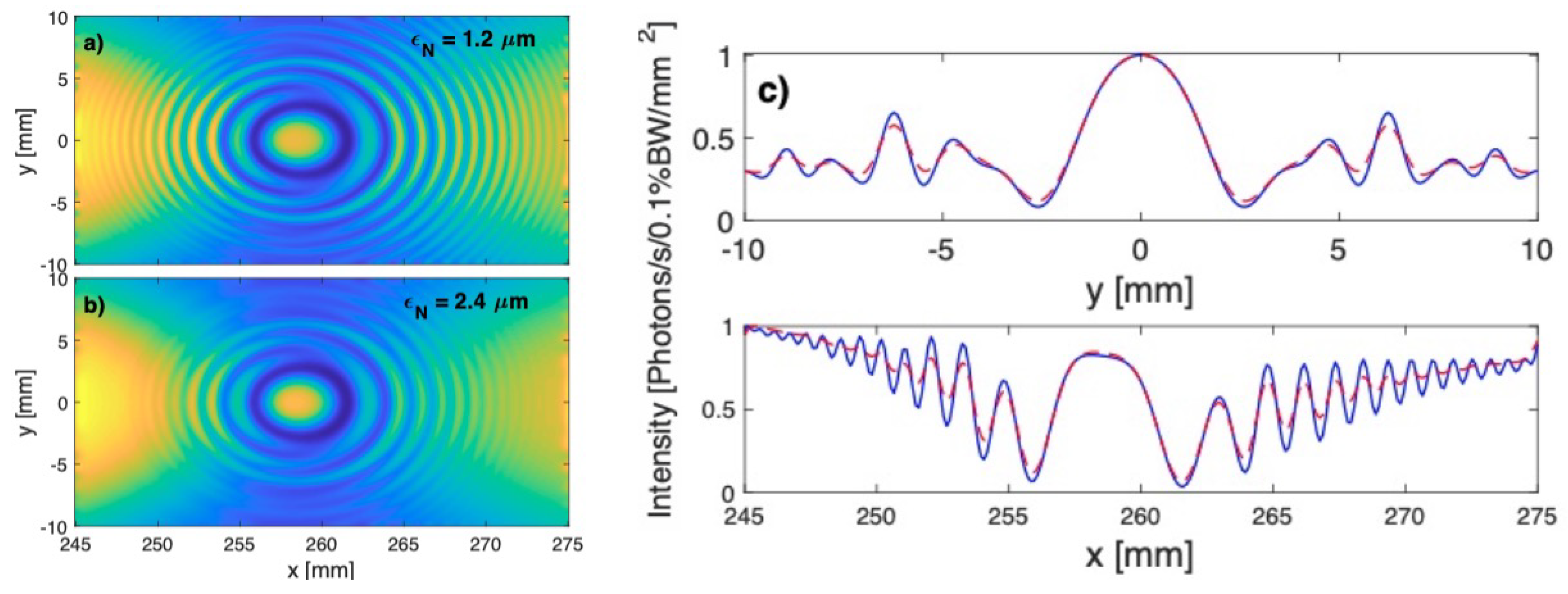
Non-destructive single-shot monitoring of beam emittance with ML-based image analysis will be carried out at FACET-II by training CNNs to predict the beam emittance, given a 2D interference pattern of edge radiation that is emitted by the electron beam as input to the ML model. This technique was previously studied in applications for the Siberia-1 electron storage ring [23] and the FERMI free electron laser [24]. We have carried out simulations of the edge radiation interference process while using the code Synchrotron Radiation Workshop (SRW) [25]. Figure 5 shows the simulation results for two different emittance beams. The blurring of the interference fringes at the larger emittance value of 2.4 m is visible to the naked eye and it is also evidenced in the lineouts that are displayed in Figure 5c. We will plan on training CNNs in a supervised learning paradigm while using multiple simulations of the edge radiation for different electron beams and train the ML-based image analysis software with simulation and experimental data. This will be accomplished starting from the photoinjector and progressively moving down the accelerator, where the alignment tolerances for the radiation pattern generated at the magnet edges become tighter as the electron beam energy increases.
3.4. Adaptive Feedback with ML for Virtual 6D Diagnostics and Control
A proof of principle adaptive model-based virtual diagnostic was demonstrated at FACET [11] and it shown to track the TCAV measurement-based LPS non-invasively based only on accelerator readouts and an energy spread spectrum of the beam. In [11], the focus was on tracking time-varying accelerator parameters and predicting one-dimensional (1D) current profiles. Recently, this approach was studied in simulation for FACET-II in which the 2D LPS was predicted and tracked based on energy spread spectrum measurements alone [13]. Figure 6 shows one simulation-based example of adaptive tuning that adjusts the parameters to match two initially different energy spread spectra, such as those that will be measured non-invasively at FACET-II, and the result is a match of the LPS and its projections.
The energy spread spectrum is measured by passing the electron bunch through a dispersive element, such as around a dipole bend so that the beam spreads transversely in the x-direction in proportion to variation in energy. The beam is then passed through a half wiggler releasing synchrotron radiation that is imaged. The radiation image is then summed vertically, giving a count at each x-location of the detector that is proportional to the number of particles that were at that offset, due to their energy offset relative to the mean energy of the bunch (see e.g., Ref. [26]).
The method works by repeatedly comparing the measured and simulated energy spread spectra and adjusting multiple components of the model in order to obtain a close match. Once the spectra are in agreement the physics model’s constraints result in a unique reconstruction of the electron bunch’s LPS. Such an adaptive model tuning-base approach in which an online model is adjusted in real time based on beam and accelerator component measurements in order to provide more accurate predictions of the beam’s 6D phase space and track both beam and accelerator parameters as they drift with time. Once such an adaptive model-based diagnostic is running, it not only provides a prediction of the 2D LPS, but of the entire 6D phase space of the beam, since it is adjusting the 6D Lucretia tracking code [4]. Figure 7 shows one example of a simulation of one section of bunch compression in FACET-II for a 2 nC beam using macroparticles. This example illustrates how the compression process, particularly in the final bunch compressor at FACET-II, results in significant changes to both the longitudinal and transverse e-beam distributions, requiring a full 6D characterization to fully capture the dynamics. If this model had been tuned online to match all possible real time diagnostics from FACET-II, then, based on previous results [11,13], it is expected to provide a virtual diagnostic of the actual beam’s 6D phase space. Furthermore, such an adaptively tuned model-based diagnostic approach will utilize all of the non-invasive diagnostics described in this paper as inputs to help more accurately match the model predictions with the actual beam. Finally, the real time beam data that are provided by an adaptive diagnostic can be used to perform real time feedback control, such as maintaining a desired phase space or to tune the beam to achieve desired custom current profiles and phase space distributions, as demonstrated in the simulation in [13].
3.5. Reinforcement Learning Controls
For FACET-II, we plan to implement and test deep reinforcement learning for the injector and linac. The reinforcement learning algorithm takes the present images of the LPS, external state information, like the present settings and virtual cathode camera images, and a target LPS image to decide what the next setting changes should be. This is then repeated until the target phase space is achieved. Initial studies of this reinforcement learning approach, as well as comparisons with approaches outlined above, will be conducted during the commissioning stage of the FACET-II accelerator, which is currently underway and the results will be reported in future publications.
4. Discussion
In this paper, we have described a suite of ML-based and adaptive virtual diagnostics, as well as adaptive and ML based controls to be used in regular operations at the FACET-II accelerator facility. These ML based tools will be used to aid machine setup, optimize beam delivery for different experiments, on-the-fly data analysis to rapidly extract beam parameters, and offline data analysis/interpretation of the experimental results. Moving from proof-of-concept demonstrations to regular deployment of these tools in accelerator operations will require addressing the major challenge of how to obtain reliable and accurate measures of the uncertainty that is associated with ML and adaptive model-based predictions. To this end, we are planning on employing the redundancy in our ML-based predictions of beam properties, e.g., using spectral data and scalar linac parameters to independently predict the beam current profile. Part of the challenge of transitioning these methods to operation will also require understanding how to effectively re-train ML models and how to couple them with adaptive feedback in the presence of machine drifts. In general, if data are collected to train a ML diagnostic with some distribution of inputs-outputs (e.g., linac phases correlating with current profiles) and this distribution changes significantly at a later time when you want to use the ML model to make a prediction, then your ML diagnostic may inacccurately predict the quantity of interest, as it has not been updated (re-trained) to reflect these distribution shifts. Progress in this area will begin by quantifying the ML-model accuracy over time, retraining the model as the observed prediction error increases beyond some acceptable threshold, and utilizing the adaptive diagnostics to guide the ML-based approaches if drift is too large or fast for re-training to keep up. Recent work on this subject has shown that ML based diagnostics can provide useful predictions (e.g., to use as a warm start for optimization), even in the presence of significant drift in machine parameters [18]. Continued investigation in this area of study is needed in order to determine how frequently re-training is required, how extensive the re-training dataset needs to be, and how this varies for smaller/larger accelerators and for predicting scalar, 1D, or 2D electron beam properties.
Author Contributions
LPS reconstruction, C.E.; Spectral Virtual Diagnostics, A.H.; edge radiation, B.O.; reinforcement learning controls, A.E.; adaptive feedback virtual diagnostics, A.S. All authors have read and agreed to the published version of the manuscript.
Funding
This research was funded in part by the U.S. Department of Energy under contract number DE-AC02-76SF00515.
Acknowledgments
The authors would like to acknowledge G. White for his contributions in setting up the start-to-end simulations of the FACET-II linac.
Conflicts of Interest
The authors declare no conflict of interest.
Abbreviations
The following abbreviations are used in this manuscript:
| ML | Machine Learning |
| TCAV | Transverse Deflecting Cavity |
| LPS | Longitudinal Phase Space |
| IP | Interaction Point |
| SVD | Spectral Virtual Diagnostic |
| PWFA | Plasma Wakefield Accelerator |
| FEL | Free Electron Laser |
| CNN | Convolutional Neural Network |
References
- Yakimenko, V.; Alsberg, L.; Bong, E.; Bouchard, G.; Clarke, C.; Emma, C.; Green, S.; Hast, C.; Hogan, M.J.; Seabury, J.; et al. FACET-II facility for advanced accelerator experimental tests. Phys. Rev. Accel. Beams 2019, 22, 101301. [Google Scholar] [CrossRef] [Green Version]
- Joshi, C.; Adli, E.; An, W.; Clayton, C.E.; Corde, S.; Gessner, S.; Hogan, M.J.; Litos, M.; Lu, W.; Marsh, K.A.; et al. Plasma wakefield acceleration experiments at FACET II. Plasma Phys. Control. Fusion 2018, 60, 034001. [Google Scholar] [CrossRef]
- Emma, C.; Edelen, A.; Hogan, M.J.; O’Shea, B.; White, G.; Yakimenko, V. Machine learning-based longitudinal phase space prediction of particle accelerators. Phys. Rev. Accel. Beams 2018, 21, 112802. [Google Scholar] [CrossRef] [Green Version]
- Tenenbaum, P. Lucretia: A Matlab-based toolbox for the modeling and simulation of single pass electron beam transport systems. In Proceedings of the Particle Accelerator Conference, Knoxville, TN, USA, 16–20 May 2005; pp. 4197–4199. [Google Scholar]
- Sagan, D. Bmad: A relativistic charged particle simulation library. Nucl. Instrum. Meth. 2006, A558, 356–359. [Google Scholar] [CrossRef]
- Borland, M. Elegant: A Flexible SDDS-Compliant Code for Accelerator Simulation. In Proceedings of the 6th International Computational Accelerator Physics Conference (ICAP 2000), Darmstadt, Germany, 11–14 September 2000. [Google Scholar] [CrossRef] [Green Version]
- De Loos, M.J.; Van der Geer, S.B. General Particle Tracer: A New 3D Code for Accelerator and Beamline Design. In Proceedings of the 5th European Particle Accelerator Conference, Sitges, Spain, 10–14 June 1996. [Google Scholar]
- Technical Design Report for the FACET-II Project at SLAC National Accelerator Laboratory. Available online: https://www.osti.gov/biblio/1340171-technical-design-report-facet-ii-project-slac-national-accelerator-laboratory (accessed on 29 January 2021).
- Scheinker, A.; Edelen, A.; Bohler, D.; Emma, C.; Lutman, A. Demonstration of model-independent control of the longitudinal phase space of electron beams in the Linac-coherent light source with Femtosecond resolution. Phys. Rev. Lett. 2018, 121, 044801. [Google Scholar] [CrossRef] [PubMed] [Green Version]
- Scheinker, A. Simultaneous stabilization and optimization of unknown, time-varying systems. In Proceedings of the 2013 American Control Conference, Washington, DC, USA, 17–19 June 2013; pp. 2637–2642. [Google Scholar] [CrossRef]
- Scheinker, A.; Gessner, S. Adaptive method for electron bunch profile prediction. Phys. Rev. Spec. Top. Accel. Beams 2015, 18, 102801. [Google Scholar] [CrossRef] [Green Version]
- Scheinker, A.; Hirlaender, S.; Velotti, F.M.; Gessner, S.; Della Porta, G.Z.; Kain, V.; Goddard, B.; Ramjiawan, R. Online multi-objective particle accelerator optimization of the AWAKE electron beam line for simultaneous emittance and orbit control. AIP Adv. 2020, 10, 055320. [Google Scholar] [CrossRef]
- Scheinker, A.; Gessner, S.; Emma, C.; Edelen, A.L. Adaptive model tuning studies for non-invasive diagnostics and feedback control of plasma wakefield acceleration at FACET-II. Nucl. Instrum. Methods Phys. Res. Sect. Accel. Spectrometers Detect. Assoc. Equip. 2020, 967, 163902. [Google Scholar] [CrossRef]
- Sutton, R.S.; Barto, A.G. Reinforcement Learning: An Introduction; MIT Press: Cambridge, MA, USA, 2018. [Google Scholar]
- Scheinker, A.; Scheinker, D. Extremum seeking for optimal control problems with unknown time-varying systems and unknown objective functions. Int. J. Adapt. Control. Signal Process. 2020. [Google Scholar] [CrossRef]
- Wu, J.; Huang, X.; Raubenheimer, T.; Scheinker, A. Recent On-Line Taper Optimization on LCLS. In Proceedings of the 38th International Free Electron Laser Conference, (FEL’17), Santa Fe, NM, USA, 20–25 August 2017; JACOW: Geneva, Switzerland, 2018; pp. 229–234. [Google Scholar]
- Bruchon, N.; Fenu, G.; Gaio, G.; Lonza, M.; O’Shea, F.H.; Pellegrino, F.A.; Salvato, E. Basic Reinforcement Learning Techniques to Control the Intensity of a Seeded Free-Electron Laser. Electronics 2020, 9, 781. [Google Scholar] [CrossRef]
- Edelen, A.; Cropp, E.; Emma, C.; Hanuka, A. Machine Learning-Based Tuning of the Round-to-Flat Beam Transform at the UCLA Pegasus Photoinjector, in preparation. Available online: https://www.preprints.org/manuscript/202101.0115/v1 (accessed on 29 January 2021).
- Hanuka, A.; Emma, C.; Maxwell, T.; Fisher, A.; Jacobson, B.; Hogan, M.J.; Huang, Z. Accurate and confident prediction of electron beam longitudinal properties using spectral virtual diagnostics. arXiv 2020, arXiv:2009.12835. [Google Scholar]
- Wesch, S.; Schmidt, B.; Behrens, C.; Delsim-Hashemi, H.; Schmüser, P. A multi-channel THz and infrared spectrometer for femtosecond electron bunch diagnostics by single-shot spectroscopy of coherent radiation. Nucl. Instrum. Methods Phys. Res. Sect. Accel. Spectrometers Detect. Assoc. Equip. 2011, 665, 40–47. [Google Scholar] [CrossRef] [Green Version]
- Maxwell, T.J.; Behrens, C.; Ding, Y.; Fisher, A.S.; Frisch, J.; Huang, Z.; Loos, H. Coherent-Radiation Spectroscopy of Few-Femtosecond Electron Bunches Using a Middle-Infrared Prism Spectrometer. Phys. Rev. Lett. 2013, 111, 184801. [Google Scholar] [CrossRef] [PubMed] [Green Version]
- Loos, H.; Borden, T.; Emma, P.; Frisch, J.; Wu, J. Relative bunch length monitor for the Linac Coherent Light Source (LCLS) Using Coherent Edge Radiation. In Proceedings of the 2007 IEEE Particle Accelerator Conference (PAC), Albuquerque, NM, USA, 25–29 June 2007. [Google Scholar]
- Chubar, O. Determining electron beam parameters from edge radiation measurement results on Siberia-1 storage ring. In Proceedings of the Particle Accelerator Conference, Dallas, TX, USA, 1–5 May 1995. [Google Scholar] [CrossRef] [Green Version]
- Fiorito, R.; Shkvarunets, A.; Castronovo, D.; Cornacchia, M.; Di Mitri, S.; Kishek, R.; Tschalaer, C.; Veronese, M. Noninvasive emittance and energy spread monitor using optical synchrotron radiation. Phys. Rev. ST Accel. Beams 2014, 17, 122803. [Google Scholar] [CrossRef] [Green Version]
- Chubar, O.; Elleaume, P. Accurate and efficient computation of synchrotron radiation in the near field region. In Proceedings of the 6th European Conference, EPAC’98, Stockholm, Sweden, 22–26 June 1998; p. 1177. [Google Scholar]
- Seeman, J.; Brunk, W.; Early, R.; Ross, M.; Tillmann, E.; Walz, D. SLC Energy Spectrum Monitor Using Synchrotron Radiation; Stanford Linear Accelerator Center: Menlo Park, CA, USA, 1986. [Google Scholar]
Figure 1.
Schematic of the planned virtual diagnostic suite and ML driven controls at FACET-II.

Figure 2.
Example shots from numerical simulation of the FACET-II two-bunch operation mode with nominal jitter values that are given in Table 1. The beam parameters are 2 nC charge and 10 GeV energy. The ML model accurately predicts the LPS distribution including chirp, time separation and bunch charge ratio. The current profile matches well with what is measured on the Transverse Deflecting Cavity (TCAV). This may deviate from the true current profile at the interaction point (IP) due to resolution limits of the TCAV for some high current shots, as shown in Figure 3.

Figure 3.
(a–e) Single shot comparisons of the current profiles obtained from the simulated TCAV images and those calculated directly from the macroparticle distribution in simulation dumped at the IP. The shots match those displayed in (f,g) Comparison of the peak current measured by the TCAV vs. at the IP for the drive and witness beam. The plots show that the TCAV measurement underestimates the peak current value and smears out some details of the current distribution for the very short bunches that will be produced at FACET-II.

Figure 4.
(a) Single shot current profile at the experimental IP of high and low peak current profile that would be appear similar on the TCAV and (b) their matching spectrum. (c) Fraction of shots that are within the TCAV resolution for various frequency bands. (d) Maximum predicted TCAV current vs integrated spectral intensity that was optimized to maximize the fraction of shots in (c). The corresponding maximum IP current is shown in the colorbar.

Figure 5.
(a,b) Examples of edge radiation interference patterns for beams of different emittance at 1 nC charge, 135 MeV beam energy with corresponding lineouts. (c) The interference pattern will be used as input to a Convolutional Neural Network (CNN) based image analysis, which will determine the beam emittance from the two-dimensional (2D) images in real-time.

Figure 6.
Simulation-based demonstration of adaptive tuning-based phase space diagnostic. Adaptively tuning the model to match a measured energy spread spectrum (A). Once the spectrum matches the LPS is uniquely reconstructed (B). Projection onto the z-axis gives an accurate diagnostic of the current profile (C). Projection onto the E-axis gives an accurate diagnostic of the energy profile (D).

Figure 7.
Simulation results showing the 6D phase space evolution of electron bunch compression in FACET-II. Axes are shown with arbitrary units with the same ranges before and after compression to show the difference.
Figure 7.
Simulation results showing the 6D phase space evolution of electron bunch compression in FACET-II. Axes are shown with arbitrary units with the same ranges before and after compression to show the difference.


Table 1.
Linac and e-beam parameters scanned in the 3125 simulations of the FACET-II accelerator. The ranges are chosen closely based on the jitter parameters from the FACET-II TDR [8]. The diagnostics fed to the ML model include random errors introduced artificially to approximate the measurement accuracy present in the accelerator.
| Simulation Parameter Scanned | Range | Nominal Value |
| L1 & L2 phase [deg] | ±0.25 | −20.75, −39.9 |
| L1 & L2 voltage | ±0.1% | 216.48 MV & 5.23 GV |
| Bunch Charge [%] | ±1 | 2 nC |
| Input to ML model | Accuracy | |
| L1 & L2 phase [deg] | ±0.25 | - |
| L1 & L2 voltage [%] | ±0.05 | - |
| at BC (11, 14, 20) [kA] | ±(0.25, 1,5) | - |
| Beam centroid BC (11, 14) [m] | N/A | - |
Publisher’s Note: MDPI stays neutral with regard to jurisdictional claims in published maps and institutional affiliations. |
© 2021 by the authors. Licensee MDPI, Basel, Switzerland. This article is an open access article distributed under the terms and conditions of the Creative Commons Attribution (CC BY) license (http://creativecommons.org/licenses/by/4.0/).
Share and Cite
MDPI and ACS Style
Emma, C.; Edelen, A.; Hanuka, A.; O’Shea, B.; Scheinker, A. Virtual Diagnostic Suite for Electron Beam Prediction and Control at FACET-II. Information 2021, 12, 61. https://doi.org/10.3390/info12020061
AMA Style
Emma C, Edelen A, Hanuka A, O’Shea B, Scheinker A. Virtual Diagnostic Suite for Electron Beam Prediction and Control at FACET-II. Information. 2021; 12(2):61. https://doi.org/10.3390/info12020061
Chicago/Turabian StyleEmma, Claudio, Auralee Edelen, Adi Hanuka, Brendan O’Shea, and Alexander Scheinker. 2021. "Virtual Diagnostic Suite for Electron Beam Prediction and Control at FACET-II" Information 12, no. 2: 61. https://doi.org/10.3390/info12020061
Note that from the first issue of 2016, this journal uses article numbers instead of page numbers. See further details here.