Missing Data Imputation in Internet of Things Gateways

Abstract

In an Internet of Things (IoT) environment, sensors collect and send data to application servers through IoT gateways. However, these data may be missing values due to networking problems or sensor malfunction, which reduces applications’ reliability. This work proposes a mechanism to predict and impute missing data in IoT gateways to achieve greater autonomy at the network edge. These gateways typically have limited computing resources. Therefore, the missing data imputation methods must be simple and provide good results. Thus, this work presents two regression models based on neural networks to impute missing data in IoT gateways. In addition to the prediction quality, we analyzed both the execution time and the amount of memory used. We validated our models using six years of weather data from Rio de Janeiro, varying the missing data percentages. The results show that the neural network regression models perform better than the other imputation methods analyzed, based on the averages and repetition of previous values, for all missing data percentages. In addition, the neural network models present a short execution time and need less than 140 KiB of memory, which allows them to run on IoT gateways.

1. Introduction

Internet of Things (IoT) systems rely on data collected by different end devices such as activity trackers and weather instruments [1,2,3,4]. In general, these systems depend on data analytics applications that use end device data to perform decision making. For example, a smart city can use sensors that collect rainfall data and send these to emergency-management applications [2]. Another example is a smart manufacturing application that can gather industrial sounds to detect machine faults and perform corrective maintenance [5].

The infrastructure of an IoT system is composed of end devices, gateways, and application servers [6]. end devices have sensors that monitor a specific environment or situation and send the data to an application server through a gateway. On the one hand, end devices often have limited computing and power resources. On the other hand, gateways have better resource provisioning and are responsible for connecting end devices to the Internet. Hence, the edge of an IoT system is composed of end devices and a gateway. Application servers, in turn, are usually located in the Cloud and have high computing power. Therefore, they run applications to analyze data and to provide intelligent services to the users [4].

The ability of IoT systems to make reliable decisions highly depends on the quality of collected data. However, end devices may fail to send data to the gateway due to networking problems or hardware malfunction. Consequently, some sensor measurements may not reach the server, reducing applications’ reliability. For example, missing data can impact statistical estimation such as means and variances [7]. The IoT system must thus be able to identify missing data and perform the appropriate corrections.

Usually, the gateway groups the data received from the end devices into records. Each record contains measurements from different sensors. For instance, a record may have a timestamp and values of atmospheric pressure, temperature, and relative humidity in weather-monitoring systems. If the record for a given timestamp lacks at least one sensor measurement, this record is considered incomplete. However, most data analysis applications only work with complete records [8,9]. In this context, the application server typically discards incomplete records received from the IoT gateway. However, depending on the amount of missing data, the database might suffer a significant reduction. As a result, discarding an entire record may reduce the reliability of data analysis applications. A better approach to ensure high-quality services is to impute the missing measurements into the record, in order to complete the application’s viewpoint [10].

This work addresses data imputation techniques in IoT systems that apply machine learning and regression analysis. These techniques can run on the application server or the IoT gateway. The first option leverages the high computing power available in the Cloud. However, it requires modifying the application. As different IoT data analysis applications run through Web services [11], this option may be difficult to implement. Running the imputation on the IoT gateway can solve this issue since it hides the missing data problem from the application. Furthermore, gateways are on the edge of IoT systems, close to the end device. Hence, imputing data on the edge is essential to real-time applications that need end device actuation [12,13].

Despite its advantages, missing data imputation on the edge needs to cope with a lower computing capacity than a Cloud solution. In this context, this work proposes a lightweight mechanism to impute data on IoT gateways. Our mechanism uses a neural network to apply regression techniques and estimate the missing data. Consequently, the IoT gateway sends complete records to the application server. To the best of our knowledge, there is no other work in the literature that proposes imputation techniques considering resource-constrained devices [10,14,15,16,17,18,19,20,21,22]. As a result, most related work does not analyze their proposals’ execution time and memory footprint.

This article is an extension of our previous work [23], in which we propose two neural network models. We thus evaluated our proposal using real weather data collected during six years in Rio de Janeiro. More specifically, we used measurements of atmospheric pressure, temperature, and relative humidity. We artificially removed a controlled amount of data and evaluated the estimation’s RMSE and coefficient of determination ($R^2$). We compared our approach with a simple method of repeating the previous value to estimate the missing one. The results show that the proposed neural network models perform better than the other methods for different percentages of missing data. The estimated values are close to that of the actual sensor measurement, presenting a $R^2$ higher than 0.92. Furthermore, we employed a Raspberry Pi Model B to show that the models use less than 140 KiB of memory, regardless of the percentage of missing data, and have a short execution time. Therefore, the proposed mechanism is suitable for resource-constrained devices such as those employed on IoT gateways.

Compared to our previous work [23], we provide a more detailed analysis of the proposed model. One significant improvement is that this extension adds two other methods to the analysis. Each method employs the same inputs as one of our two neural network models. However, for each one, the estimated value is the average of the inputs. Our idea was to use these methods to verify whether our neural networks models do more than simply average the input values. We show that these two methods have worse RMSE and $R^2$ results than the simple previous value repetition used in [23]. These results emphasize the importance of employing a neural network to impute missing data. This extension also adds, for all methods, scatter plots that capture the relationship between the estimated values and the original ones. Their results show that our neural network models provide estimated values closer to the original one than the other methods.

This article is organized as follows. Section 2 describes the related work. Then, Section 3 and Section 4 detail our proposal and the evaluation methodology, respectively. Section 5 shows the performance results, comparing our method with baselines, while Section 6 discusses our findings. Finally, Section 7 concludes this work and describes future work.

2. Related Work

In data analysis, several algorithms do not correctly perform when there are missing data in the dataset [8,9,16,24]. Therefore, the missing data problem is one of the biggest challenges for IoT-based systems [9]. A typical approach to solve this problem consists of eliminating incomplete records, that is, records with one or more attributes with missing values. However, this approach reduces the amount of available data, and as a consequence, the application may misinterpret the data [17]. This problem thus justifies the need for imputing missing data with appropriated values.

A widely used method replaces the missing value with the average of all non-missing values received for such an attribute in the dataset. However, this method distorts the attribute’s probability distribution [24] and does not perform well in most cases [14]. Other simple methods include replacing the missing value with a random value, the median of existing values, or zeros. Furthermore, there are more complex imputation methods based on statistics (i.e., expected maximization (EM) [8]), optimization (i.e., genetic algorithm (GA) [10]), and machine learning approaches (i.e., K-nearest neighbors (K-NN) [25], support vector machine (SVM) [26], and K-means [15]). In addition, there are also hybrid approaches that mix these categories [17].

According to Yan et al. [8], IoT data have spatial and temporal correlation characteristics, which we should consider when dealing with missing data imputation. They divide missing data into three categories: missing completely at random (MCAR), missing at random (MAR), and not missing at random (NMAR). In MCAR, a missing value in an attribute occurs regardless of the other attributes and its value (e.g., a specific sensor may fail and does not collect data). In MAR, there is a relationship between the missing attribute and the available information. For example, a person may remove their smartwatch at night to charge. Thus, it does not collect their vital signs data [27]. In NMAR, the missing attribute depends on its value. For example, a person may remove their smartwatch before smoking as they do not want any sign associated with smoking to be collected [27]. The authors propose three models to solve these problems based on the context and linear mean, binary search, and Gaussian mixture model (GMM) based on expected maximization (EM). Results show that all models have high accuracy. As IoT missing data mainly occur due to sensor failures or network problems—which fits the MCAR category [19]—many works in the literature start from this premise to impute missing data [18,19,20].

The authors in [27] proposed a decision-making approach to deal with the missing data in a real-time healthcare application, using a multiple imputation approach [28]. For each missing value detected in the heart rate sensor, the application uses medical history and additional state information (i.e., sleep, light activity, vigorous activity) collected by the other sensors to estimate multiple values. Then, they aggregate these values using a weighted arithmetic mean, in which the weights are determined according to the additional state information associated with the missing heart rate. Compared to other methods, such as K-NN, autoregressive, and SVM, the proposed approach outperforms their accuracy when the missing interval is greater than 1 h.

In their work, Liu et al. [9] focused on missing data imputation with large gaps. They considered data with high seasonality and treated them as a time series. This method segments large gaps into pieces according to the desired seasonality length. For each gap, they used linear interpolation to impute missing data, and then they applied the seasonal and trend decomposition using Loess (STL). STL decomposes time series data into trend, seasonality, and remainder components. They used the seasonality to learn the repetition pattern, and the imputation result is computed by the combination of the other components. Hence, each iteration’s result is better than the previous one. This method performs better than other methods in the literature that deal with databases with large missing data gaps. The authors in [12] presented a multi-agent system (MAS) technique to impute missing values in an edge environment. More specifically, they consider IoT devices such as ad hoc sensors and mobile devices. In this approach, each device is called an agent, and the MAS allows distributing the computation among them. The agents can have fixed sensing devices or not. The former ones are divided into regions according to their dynamics, and the latter, which is usually mobile, cooperates with the agents in the same region they are. To impute a missing value, the authors computed the inverse distance weighting (IDW) interpolation and compared the result with the closest device’s value and the values of the same region. The results show that the errors between the imputed values and the values provided by the fixed agents are low in more than 70% of the simulations. However, they provide only simulation results, not showing their impact on devices with limited computing resources.

Fekade et al. [14] first used the K-means algorithm to group sensors according to their measurements’ similarities. They applied the probabilistic matrix factorization (PMF) algorithm in each group. Then, they recovered the missing values using the PMF property that obtains the original matrix by computing the product of two matrices corresponding to the measurements of neighboring sensors. This approach performs well in terms of accuracy, errors, and execution time compared to SVM and a deep neural network model. However, González-Vidal et al. [29] claimed that the PMF execution time increases as the number of missing data increases. Their work proposes a framework that imputes missing data using the Bayesian maximum entropy (BME) method. BMF is a mapping method to estimate spatial-temporal values that allow the use of multiple knowledge databases. This method uses two databases: one with statistical data and one more specific, which contains data collected by sensors with different precision. The first database is used in the maximum entropy function, and then it is combined with the specific database. This combination minimizes the quadratic squared error, resulting in the spatial-temporal mapping. The results show that this method performs better than the PMF approach, with a shorter execution time. The authors also stated, with no experimental results, that they can extend their framework to impute data in an online scenario.

Li et al. [15] proposed imputing missing data using a fuzzy K-means algorithm, in which each record has a membership function. This function describes the degree to which the record belongs to a specific cluster. Therefore, this method uses the degree information and the cluster’s centroid values to impute missing data. This approach performs better than using averages and the K-means algorithm. In Mary et al. [16], the authors first identified the sensors correlated to the sensor that was responsible for the missing data by using the Pearson correlation coefficient. Then, they replaced the missing data using the value collected at the same hour by the sensor with the highest correlation. Although these clustering algorithms performed better than some well-known methods, such as K-NN and SVM, they imputed all missing data from the database at once. Hence, they did not consider the order of the records’ timestamps. In this way, old records with missing data may remain unvalued until the algorithm runs. In addition, records received after the missing data may be used to predict a value for the respective record, which makes it unusable in online applications that consider timestamp ordering. Furthermore, these clustering approaches do not mention whether the algorithm should run whenever an incomplete record arrives at the dataset, which would increase their computational cost.

Izonin et al. [30] described a regression method based on general regression neural network (GRNN), which has three layers: input, radial, and output. First, they compute the Euclidian distance from the input array to all other training datasets samples. This result was transformed into a Gaussian distance and compared to the predicted values for evaluation. They tested this method for only one attribute of the dataset, and its results are better than for any other known methods, including AdaBoost [31] and support vector regression (SVR) [32]. However, the GRNN training may become slower depending on the amount and structure of the training samples. Turabieh et al. [21] used the deep learning model layered recurrent neural network (L-RNN) to dynamically predict the missing values. As soon as their method receives a record, it is inserted in the training dataset if such a record is complete. If the record has missing values, they used L-RNN to impute the value and then insert it in the training dataset. Therefore, records with imputed values are used for training and for producing new predictions. These approach results are better than K-NN and a decision tree. Zhang et al. [20] recovered missing data time series in wireless sensors networks using a long short-term memory (LSTM) neural network. In addition, they proposed a sliding window algorithm to produce more training samples from small datasets. This approach performs better than expected maximization (EM) and autoregressive integrated moving average (ARIMA) [33], for example. However, it uses both old and future data to predict the current missing value.

Guzel et al. [17] proposed models using LSTM and fuzzy logic. They assumed that a record has three attributes and predicts the missing value using the other two attributes received in the same timestamp. In [19], Kök et al., used the same models as those proposed by [17], but they implemented them in edge and Cloud devices. Their goal was to have a low delay and efficient use of the network’s bandwidth. However, both [17] and [19] only work with one missing attribute at a time. Nikfalazar et al. [18] used decision trees and fuzzy K-means algorithms. The decision trees compute the first predictions for a missing value, and then these values are updated using the fuzzy K-means algorithm. The fuzzy K-means always uses the last predictions as input values until a stop criterion is reached. This method generates good predictions in different databases. However, it takes more execution time than others in the literature. Al-Milli et al. [10] proposed a hybrid model with a neural network and a genetic algorithm (GA) to impute missing data. The former predicts the missing values, while the GA is used to optimize the neural network’s weight. The authors compared the application performance with missing data and after using their hybrid imputation method. Therefore, they showed that missing data imputation helps improve the application’s result. Wang et al. [34] proposed a missing data imputation method based on functional dependencies and association rules. The authors first modeled a big data schema in which the record’s attributes describe a specific object. They focused on finding the relationship between these attributes and the sequence of events that frequently occurred since knowing the patterns in the sequences helps predict their occurrence in the future. Thus, they used a probabilistic production dependency method which produces classification rules valid for a significant number of entities from a selection. Then, they used the sequence of rules to build an operator to recover the missing data. To evaluate the proposed method, the authors used a classifier built on the original dataset. Their methods performed better than the expectation-maximization (EM) and random forest (RF) methods when up to 30% of data were missing. For higher percentages, these lose to EM. Regarding the time analysis, their approach has better results than SVM, EM, and association rules. The main difference between [34] and our work is that they did not address an online scenario, thus using all the data available in the dataset.

Most related work has exclusively focused on the prediction quality and did not consider computational resources requirements such as memory and processing. This concern is crucial in an IoT environment since the hardware usually has limited resources. Only a few of them [14,17,18,29,30,34] considered the execution time of the proposed methods. The works in [12,19,27,29] claimed that their methods might execute in an edge computing device, such as IoT gateways or IoT devices, but they did not provide experimental results. However, none of the works analyzed the amount of memory that the methods consumed. In addition, most works considered that all the dataset was available, so in order to impute a missing value, these methods can use values received after the missing value timestamp.

Table 1. Characteristics of related work.

Paper	Computation	Uses Neighbor Sensors’ Data	Used Approach	Uses Only Previous Data	Analyzes Time	Analyzes Memory
[8]	Not defined	-	Statistical (GMM and EM)	-	-	-
[9]	Cloud	-	Statistical (STL)	-	-	-
[12]	Edge	✓	Statistical	✓	-	-
[16]	Not defined	✓	Statistical (PCC)	-	-	-
[27]	Edge and Cloud	✓	Statistical	-	-	-
[28]	Not defined	-	Statistical	-	-	-
[29]	Edge and Cloud	✓	Statistical (BME)	-	✓	-
[30]	Not defined	-	Machine learning (GRNN)	-	✓	-
[14]	Not defined	-	Machine learning (K-means) and Statistical (PMF)	-	✓	-
[15]	Not defined	✓	Machine learning (fuzzy K-means)	-	-	-
[17]	Not defined	✓	Machine learning (recurrent neural network) and fuzzy logic	-	✓	-
[18]	Not defined	✓	Machine learning (decision tree and Fuzzy K-means)	-	✓	-
[19]	Edge and Cloud	✓	Machine learning (recurrent neural network) and fuzzy logic	-	-	-
[20]	Not defined	-	Machine learning (recurrent neural network)	-	-	-
[21]	Not defined	✓	Machine learning (recurrent neural network)	-	-	-
[34]	Not defined	-	Functional dependencies and association rules	-	✓	-
[10]	Not defined	-	Machine learning (recurrent neural network) and optimization (genetic algorithm)	-	-	-
This work	Edge	-	Machine learning (neural network—MLP)	✓	✓	✓

compares the main characteristics of the mentioned works. Unlike literature approaches, this work imputes missing data on the fly, namely, as soon as they arrive at the IoT gateway and before forwarding the record to the application server. In this way, only data received before the missing data are available to predict such a value. Another critical difference is that we measure the execution time and the amount of memory used for the methods since our approach runs at IoT gateways.

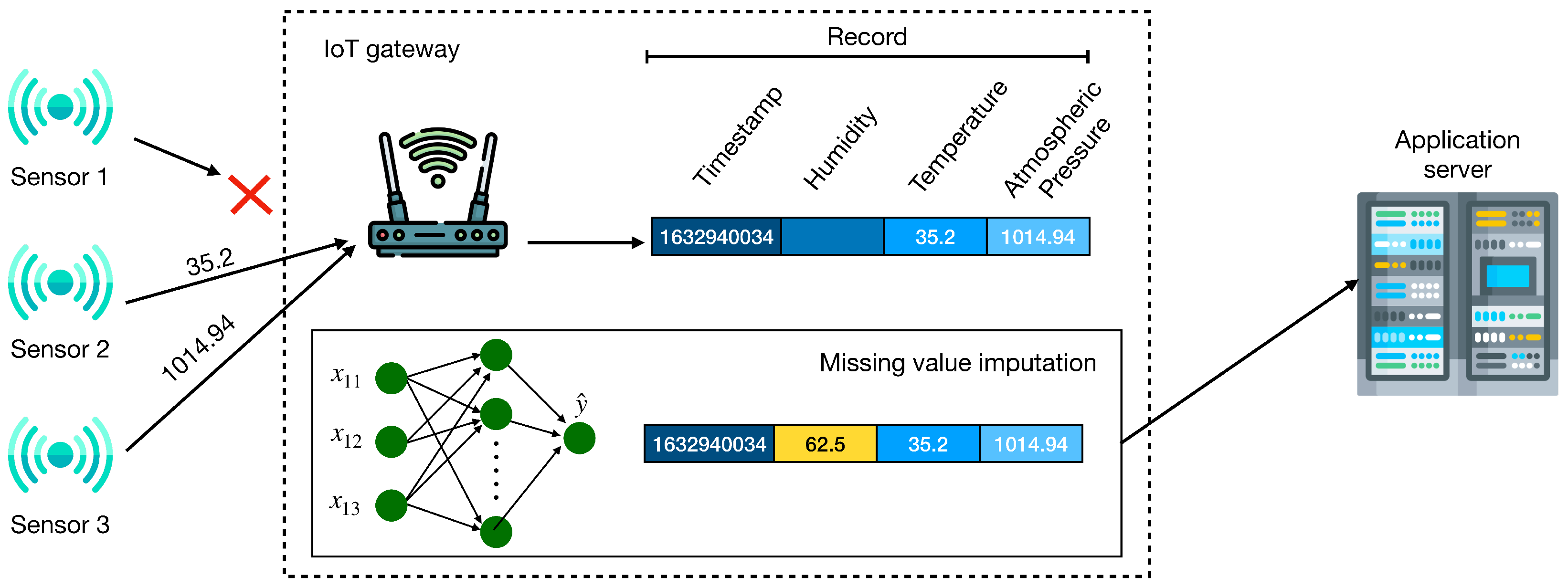
3. Imputation Method Based on Neural Networks

In our mechanism, each IoT gateway trains a machine learning model using data sent by sensors and then uses such a model to impute missing data. We trained our models in the gateway to allow all the processing to be on the network’s edge, so it has more autonomy to train and impute missing data without waiting for a Cloud response to update its model. In addition, this approach reduces network overload since fewer data travel over the network to the Cloud. As IoT gateways have limited processing resources, we need a simple and fast training machine learning model.

Figure 1 shows the scenario in which our mechanism runs. Each sensor is responsible for monitoring an attribute. On a particular day and at a specific time, the sensor collects the attribute value and sends it to the gateway. The gateway then gathers the values from all sensors into a single record that corresponds to a specific timestamp. More specifically, a record is the set of attributes collected by sensors at a specific timestamp.

Due to various reasons, the gateway may not receive all attributes values collected by sensors. Hence, the record related to such a timestamp will be missing data (i.e., a lack of one or more attributes). In Figure 1, for example, Sensor 1 fails to send the humidity attribute measurement. A typical approach is to discard the entire record, but it implies discarding all other received attributes. In addition, in the case of damaged sensors, the gateway might not receive such attributes for a long time, discarding all the other measurements. Additionally, discarding the record may also make it difficult to trace back a damaged sensor. Discarding all records with at least one missing value can significantly reduce the amount of data and might deteriorate the performance of the data analysis application. Finally, it can even prevent the application from working in extreme situations in which there are insufficient records. Therefore, instead of discarding records with missing values, it is crucial to impute data with appropriated values to guarantee that the data analysis performs well.

In the scenario of Figure 1, whenever there is a missing value in the record, the gateway imputes an appropriated value. This marks such an attribute before sending it to the application server. This mark allows the application to know which values were not measured by a sensor. The gateway performs imputation even when it does not receive any attribute values for a specific timestamp. However, the gateway does not send this record to the application server since it can be useless to the data application analysis. In this way, we also avoid increasing the network load with a record with only predicted values. In this case, the imputed values are only relevant to help the gateway improve its training.

In this work, we propose a mechanism based on a regression model that uses multi-layer perceptron (MLP) [35]. As MLP is a neural network, we employ both terms as synonymous throughout the text. To predict the attribute’s measures, we implemented two different neural networks. To implement them in an IoT gateway with few resources, they needed to be simple. Therefore, these models have only one hidden layer. Hence, the hidden layer’s neurons process data received from the input layer and send them to the output layer. The models differ in the amount of input data and in the attributes they represent. Each attribute has its own neural network model and its own training set.

In order to predict a specific value, from a given timestamp $t_i$, the first neural network model, referred to as $NN1$, has as input data the values of the three timestamps immediately before $t_i$ for a specific attribute. This model has a low memory footprint since only the three previous values need to be kept in RAM. The second neural network model, referred to as $NN2$, has as input data four values for each attribute: the values of the three timestamps immediately preceding $t_i$ (exactly as $NN1$) and the measure of the same timestamp on the previous day. With this model, we want to analyze whether the measure of the previous day for the same timestamp helps predict a better result.

For implementing the MLP models, we use Scikit-learn 0.24.1 [36], a machine learning library. When using the MLP as a regression model, the activation function in the output layer is the identity function, and we minimize the squared error. As MLP is sensitive to the data scale, we have to apply a normalization function to obtain good results. To create and train an MLP model, we need to define a set of hyperparameters. We empirically chose the hyperparameters as follows. We used different hyperparameters’ combinations to train the models and then evaluate the model’s performance using the test dataset. Then, we computed the $R^2$ score and RMSE metrics using the original values of the test dataset and the predicted values. Finally, we chose the combination with the highest $R^2$ score and lower RMSE in the following experiments.

Both neural network models use the same set of hyperparameters.

Table 2. Neural network models’ hyperparameters. Adapted from [23].

Hyperparameter	Value	Hyperparameter	Value
hidden_layer_sizes	100	validation_fraction	0.1
activation	ReLU	tol	0.0001
solver	Adam	random_state	1
learning_rate_init	1	alpha	0.0001
batch_size	$min(200,n)$	beta_1	0.9
max_iter	500	beta_2	999
early_stopping	True	epsilon	1 × 10${}^{-8}$
n_iter_no_change	4	shuffle	True

shows the hyperparameters and their respective values. The hidden layer has 100 neurons and the activation function in this layer is ReLU (Agarap—“Deep learning using rectified linear units (ReLU)”, available at https://arxiv.org/abs/1803.08375—accessed on 12 October 2021), where $f\left(x\right)=max(0,x)$. ReLU returns 0 when x is negative. Otherwise, it returns the value itself. The optimization algorithm is Adam (Kingma and Ba—“Adam: A method for stochastic optimization”, available at https://arxiv.org/abs/1412.6980—accessed on 12 October 2021), since it performs well in large databases, with thousands of training samples and quickly converges. The learning rate to update the weights is constant. The $\mathit{batch}\_\mathit{size}$ hyperparameter defines the number of training samples to be used in an iteration. It is $min(200,n)$, in which n is the total number of samples. The maximum number of iterations (i.e., the number of epochs $max\_iter$) was set to 500. The $tol$ represents the tolerance for the optimization. The $early\_stopping$ hyperparameter defines that if the score does not improve by at least $tol$ for a defined number of consecutive iterations ($n\_iter\_no\_change$), the MLP considers that it has reached the convergence and then finishes the training. The proportion of training data to be used as a validation set for early stopping is 0.1. The random_state hyperparameter allows the reproducibility of the experiments. This determines the random values for weight’s initialization and bias, the separation of data into training and validation sets (if early_stopping is activated), and the batches samples. When activated, shuffle determines that the samples must be shuffled in each iteration. The alpha hyperparameter corresponds to the L2 regularization term, which applies a penalty in the optimization function to prevent model overfitting. For the Adam optimizer, the beta_1 and beta_2 hyperparameters are defined, which are the exponential decay rate for estimates of the first and second moment vector, and epsilon, which is the value for numerical stability.

4. Evaluation Methodology

This section first describes the employed dataset and then details the evaluation methodology.

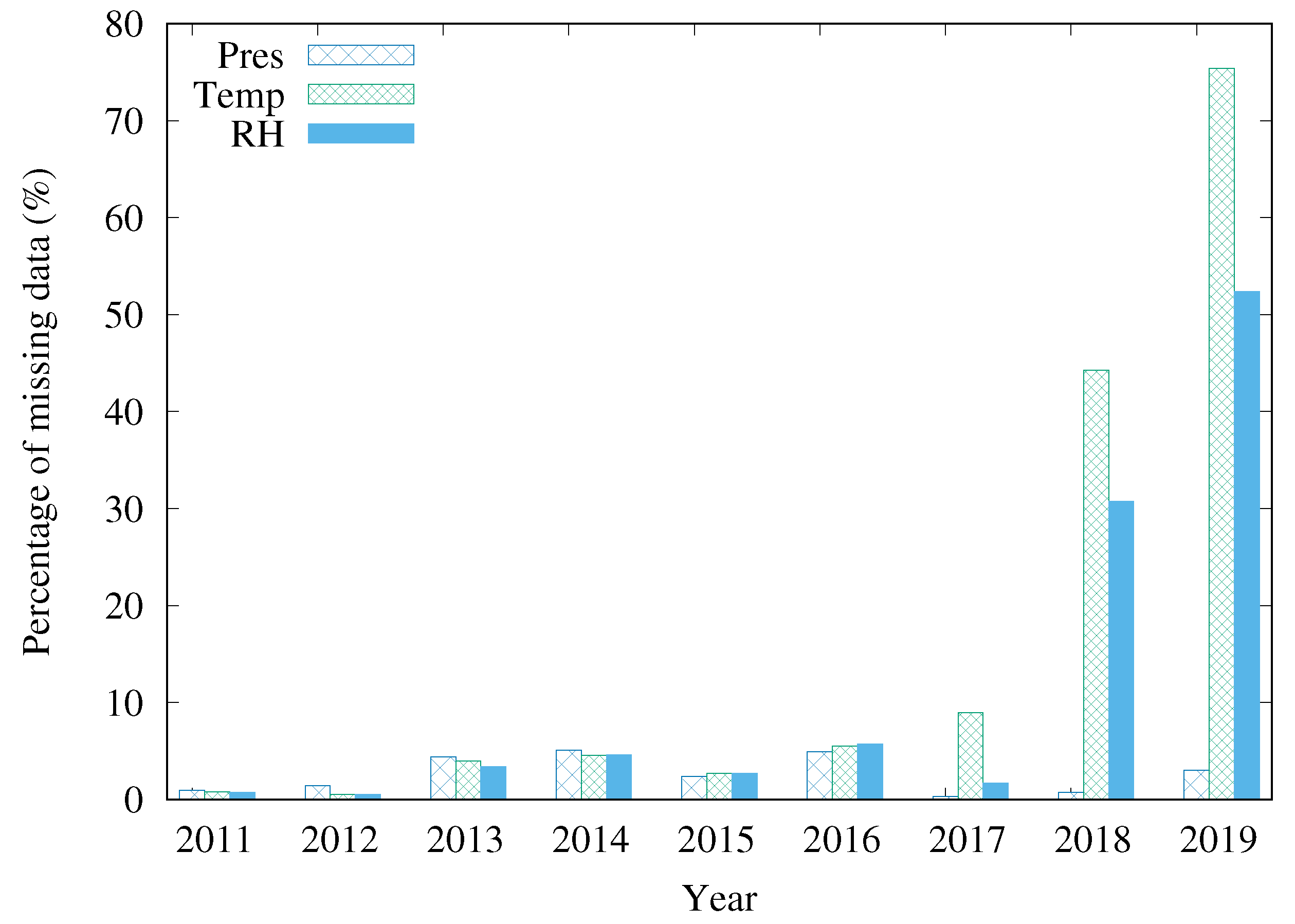
4.1. MonitorAr Dataset

In this work, we used the MonitorAr (Cityhall of Rio de Janeiro—“MonitorAr dataset”, available at https://www.data.rio/datasets/dados-horários-do-monitoramento-da-qualidade-do-ar-monitorar/explore—accessed on 16 October 2021) dataset, which contains meteorological data, measured every hour, from a station in Rio de Janeiro, located in the neighborhood of São Cristóvão. We used the atmospheric pressure (Pres) (mbar), temperature (Temp) (${}^{\circ }$C), and relative humidity (UR) (%) attributes from 2011 to 2019. The station has complete records, records with missing values in some attributes, and gaps between timestamps, i.e., hours when no data were received. To overcome this issue, we preprocessed the dataset by inserting empty records whenever a timestamp was missing. As a result, each day has 24 records (i.e., one per hour), and each year has 8760 or 8784 records, depending on whether the year is a leap year.

Figure 2 shows the missing data percentage for each attribute over the years. More precisely, it shows the number of records without a specific attribute over the total number of records expected for the year. It is possible to note that the missing data problem is serious in this station, especially from 2017 to 2019. Considering the interval from 2011 to 2019, the number of records with at least one missing attribute—not shown in this figure—represents 16.8% of the total number of records. If these incomplete records are deleted, the other sensors’ measures are lost, and the application will have fewer data to work with. This result highlights the need to impute missing data.

Our experiments consisted of varying the missing data percentage of the dataset by removing valid measures to verify the effectiveness of our models. As the missing data percentage from 2017 to 2019 is already high, it was not convenient to introduce more missing data. It would not be possible to simulate scenarios with a few missing data for these years. Therefore, our evaluation used data from period from 2011 to 2016.

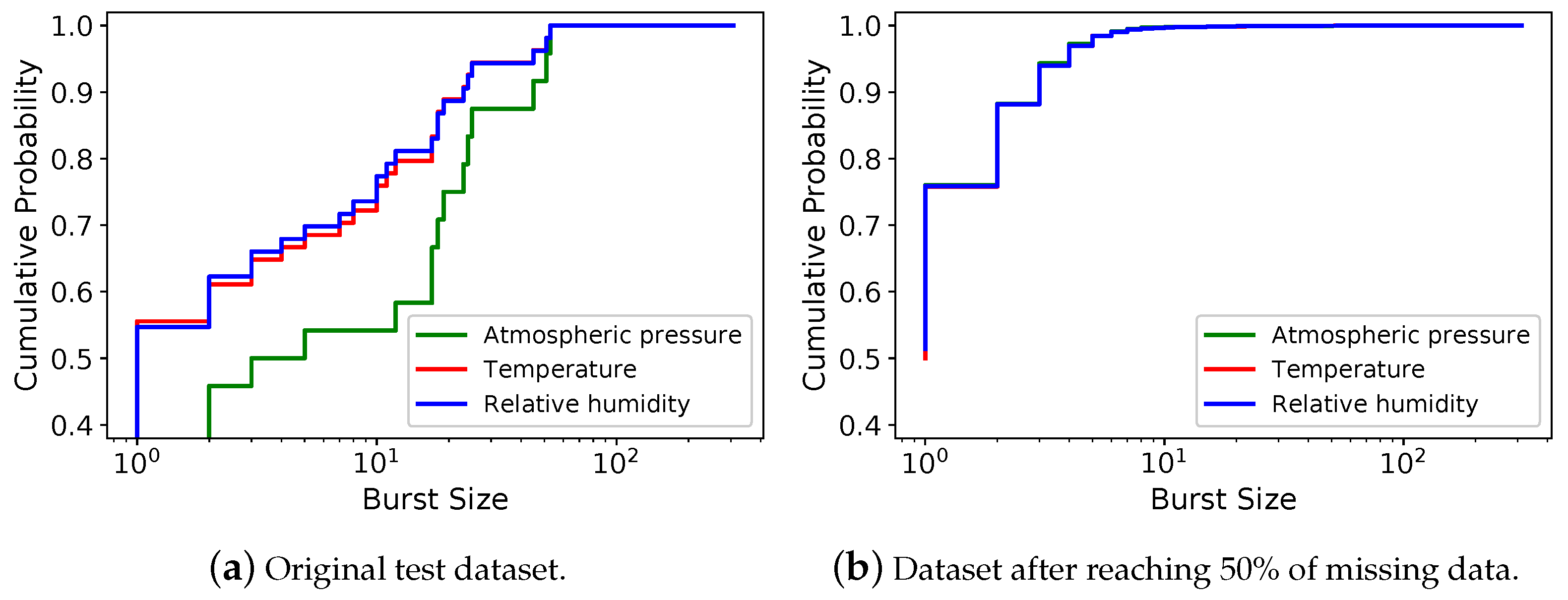
4.2. Missing Data Insertion

To evaluate our imputation method, we varied the missing data percentage in the dataset as 5%, 10%, 25% and 50%. For instance, if the dataset has 100 records, 10% of missing data means that each attribute has ten missing values. As the original dataset already has missing data, we first verify how much data are missing for each attribute. Then, we remove the necessary amount to achieve the desired missing data percentage. After defining the number of values to be removed, we randomly chose them using a uniform distribution. For all missing data percentages, we performed this process 50 times. We then divided the dataset into training and test datasets and standardized the datasets to have zero mean and unit variance. The training dataset has data from 2011 to 2014, and the testing dataset has data from 2015 to 2016.

Missing data can occur as isolated or in bursts. The burst size corresponds to how many consecutive missing values happen for one attribute. Hence, an isolated loss is a burst of size one. Figure 3a shows the cumulative probability for each burst size of the original test dataset. The majority of missing data burst sizes are small. However, there are bursts with more than 100 consecutive missing values.

Figure 3b shows the cumulative probability of the burst size of one sample of the test dataset after removing values to reach 50% of missing data. The burst sizes of the attributes are very close to each other. The probability of having an isolated loss is approximately 76%, greater than the original test dataset probability( 0.56). This behavior was expected since we selected data to remove using a uniform random distribution. Considering all 50 samples, even after removing data from the dataset, bursts of sizes up to 3 represent most of the missing data. This behavior also happens in the original test dataset for the temperature and relative humidity attributes.

This analysis is interesting because the burst size can impact the imputation method prediction quality. Therefore, an imputation method should be able to handle different missing data burst sizes.

4.3. Baseline Imputation Methods

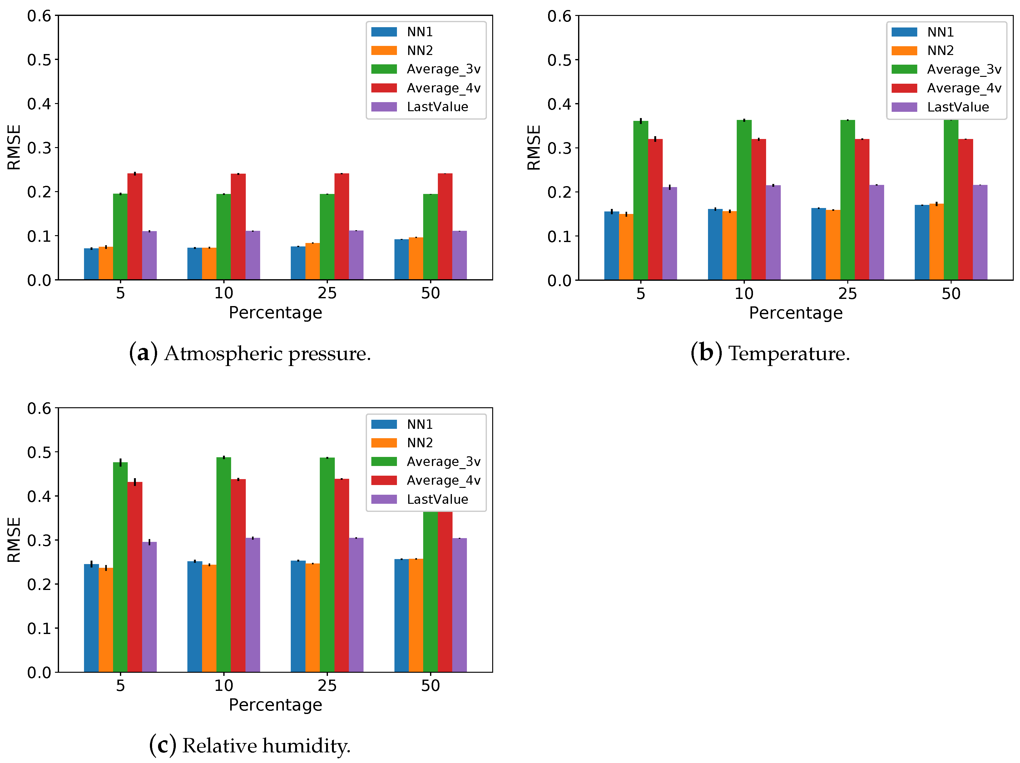
We compared the neural network models with the following baseline methods:

• Average ($Average$)—we replace the missing value with the average of all previously received values for the corresponding attribute;
• Average of $NN1$ input data ($Average\_3v$)—we replace the missing value with the average of $NN1$ inputs (i.e., the average of the last three measures of the corresponding attribute);
• Average of $NN2$ input data ($Average\_4v$)—we replace the missing value with the average of $NN2$ inputs (i.e., the average of the last three measures and the previous day’s value at the same hour of the corresponding attribute);
• Repetition of the last received value ($LastValue$)—we replace the missing value with the last received value of the corresponding attribute.

The $Average$ baseline is a simple and widely used imputation method. However, in our experiments, this method had the worst performance, as expected [14], since it distorts the attribute probability distribution. Thus, for better conciseness, we omit its results in this work. The $Average\_3v$ and $Average\_4v$ methods were chosen to verify whether it is really necessary to create a neural network model to impute missing data or if the simple averages of $NN1$ and $NN2$ input data already produce good predictions. The $LastValue$ is the simplest method since it only needs to store one value and repeat it once. Due to its simplicity, the $LastValue$ is used as a baseline method for the computational resource analysis.

5. Results

Our experiments used MonitorAr data from 2011 to 2014 to train the neural network models. We evaluated all imputation methods using data from 2015 and 2016. Each method predicted a value for the missing data as soon as the record arrived at the gateway, respecting timestamp ordering. Therefore, the imputation only uses records received before the current timestamp. All results were expressed with the mean of 50 samples and a confidence interval of 95%, although imperceptive in some figures.

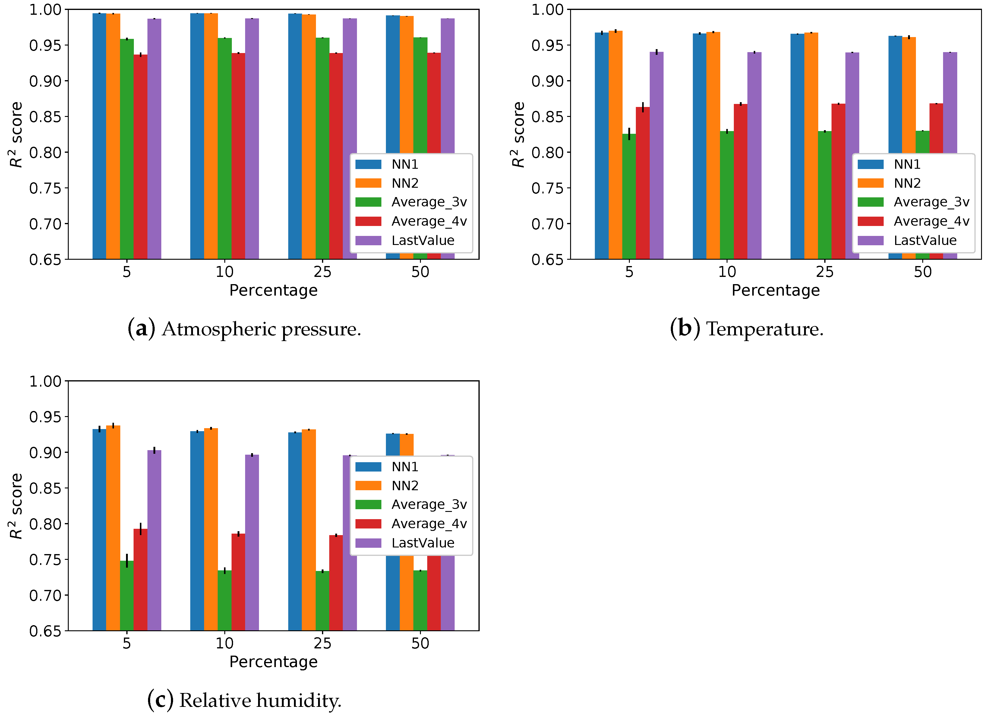
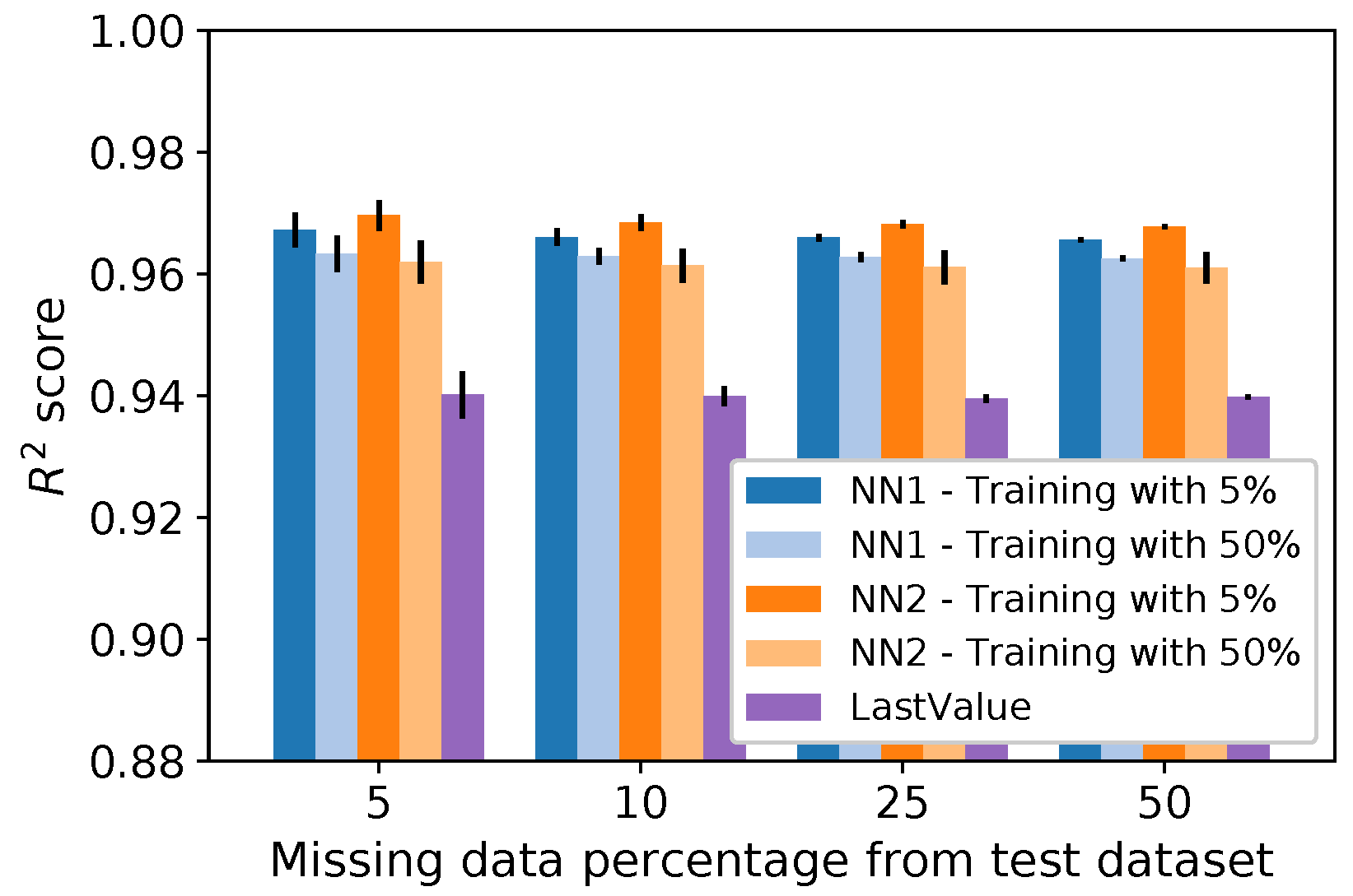
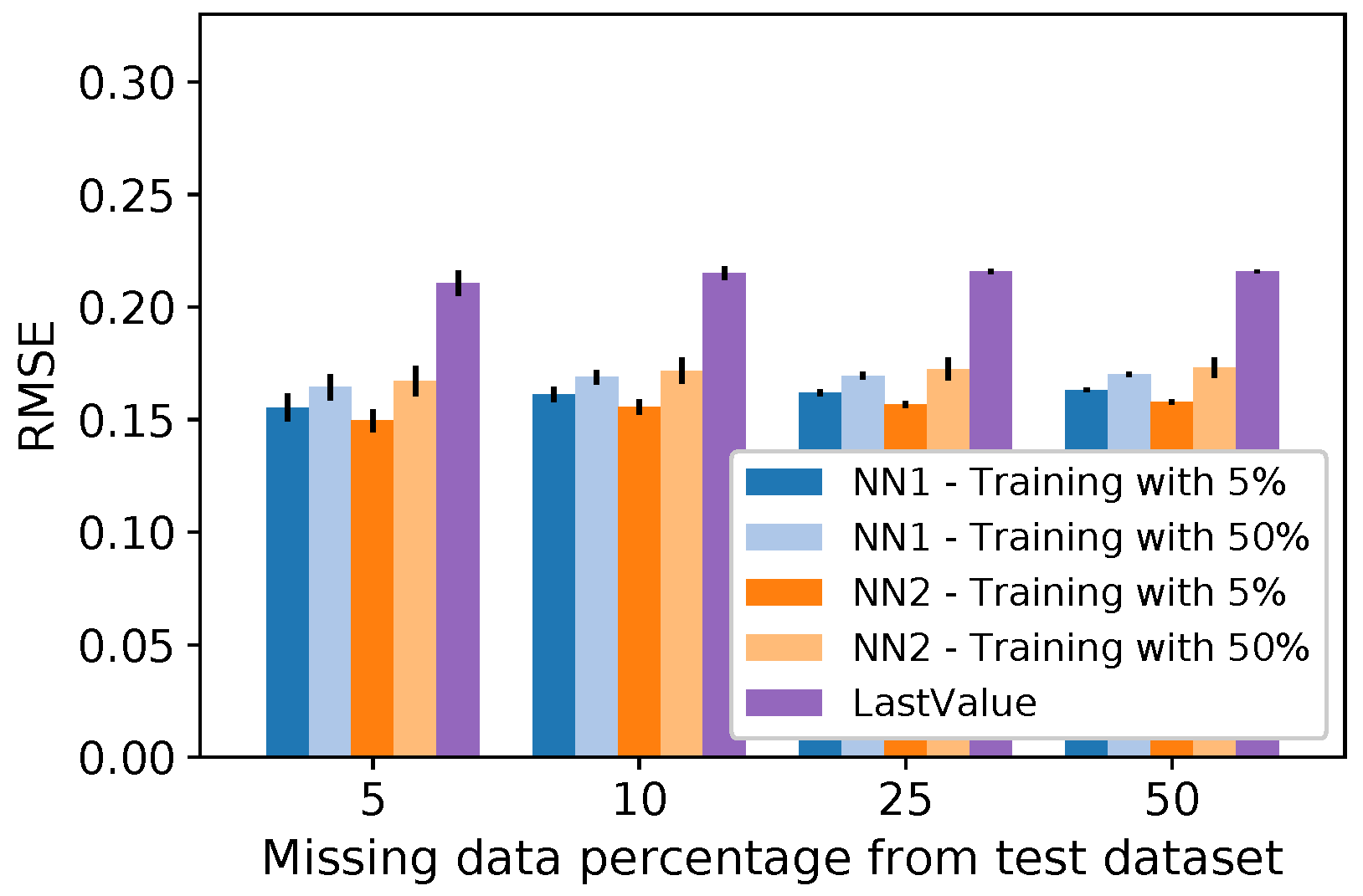
5.1. Imputation Methods Performance

Our performance evaluation uses the coefficient of determination ($R^2$ score) and the root mean squared error (RMSE). The $R^2$ score indicates how well the model fits the data and is defined as follows:

$$R^2(y,\hat{y})=1-\frac{{\sum }_{i=1}^n{(y_i-{\hat{y}}_i)}^2}{{\sum }_{i=1}^n{(y_i-\overline{y})}^2},$$

(1)

where n is the number of records, $y_i$ is the actual value of record i, $\hat{y}$ is the predicted value for this record, and $\overline{y}$ is the average of all records. Note that ${\sum }_{i=1}^n{(y_i-{\hat{y}}_i)}^2$ is the sum of the error’s squares. Its results vary from zero to one, with zero being the worst possible value and one being the best value.

The RMSE is a metric used to measure the model’s errors. This metric is always non-negative, with zero being the best possible value. The RMSE is defined as follows:

$$\mathrm{RMSE}(y,\hat{y})=\sqrt{\frac{1}{n}\sum _{i=1}^n{(y_i-{\hat{y}}_i)}^2},$$

(2)

Figure 4 shows the $R^2$ scores of the imputation methods when varying the missing data percentage on training and testing sets simultaneously. We evaluated the performance for atmospheric pressure, temperature, and humidity attributes.

$NN1$, $NN2$ and $LastValue$ reach high $R^2$ scores for the atmospheric pressure (Figure 4a). The $LastValue$ achieves a good performance in this attribute since the atmospheric pressure has a low variation for near instants in time. However, this characteristic does not apply to the other attributes. For temperature (Figure 4b) and relative humidity (Figure 4c), the difference between the neural network models and the $LastValue$ is more significant than with the atmospheric pressure.

Figure 4a also shows that using the measure at the same hour of the previous day does not help $NN2$ in the prediction. $NN1$ is thus simpler, and its results are statistically close to $NN2$. Unlike the neural network models, the $Average\_4v$ performs better than $Average\_3v$ for temperature and humidity attributes. However, results of $Average\_3v$ and $Average\_4v$ are worse than their corresponding neural network models ($NN1$ and $NN2$). It justifies using the proposed neural networks to predict missing data instead of using a simple average.

Figure 5 complements the previous results, presenting the calculated RMSE for each attribute when we varied the missing data percentage. $Average\_3v$ and $Average\_4v$ have the worst RMSE values for all attributes. The $LastValue$ method performed better than $Average\_3v$ and $Average\_4v$. The RMSE results for $LastValue$ are still worse than the neural network models for all attributes. Finally, Figure 5 shows that the RMSE values of the neural network models (i.e., $NN1$ and $NN2$) are close to each other for all attributes and missing data percentages. Therefore, these results reinforce that adding one more input datum does not help the $NN2$ model.

Figure 4 and Figure 5 show that the missing data percentage has a low impact on the performance of the methods since the $R^2$ and RMSE values did not vary significantly as the missing data percentage increased. This behavior was expected since the missing data percentage insertion follows a uniform distribution. Consequently, there are still a lot of isolated losses. As shown in Figure 3b, the probability of an isolated loss is higher than burst losses, which may prevent the error propagation.

Another way to compare the imputation methods is to analyze the relationship between the original and predicted values. In a perfect model, these values must be the same. Figure 6 shows this relationship for the relative humidity attribute of one sample, where the x axis presents the original values and the y axis presents the predicted values. The plotted values refer to the missing data randomly inserted to reach 50% of missing data on the dataset. Furthermore, they are in their original magnitude. Namely, they are not transformed by the standard normal distribution. It is possible to see that, with $NN1$ and $NN2$ methods, the points are more concentrated in the ideal line when compared to the other methods. We present a sample of the humidity attribute since its results are worse than the others’ attributes. However, for all samples and attributes, the neural networks perform better than the other methods.

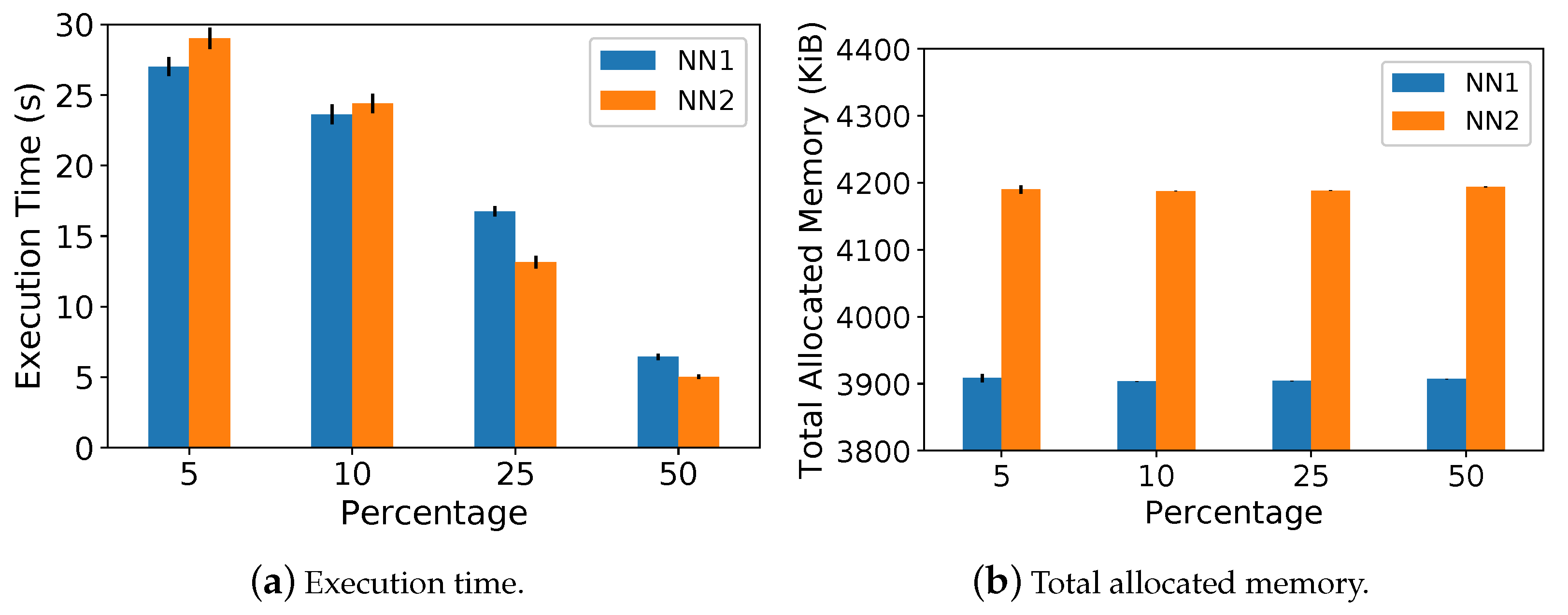
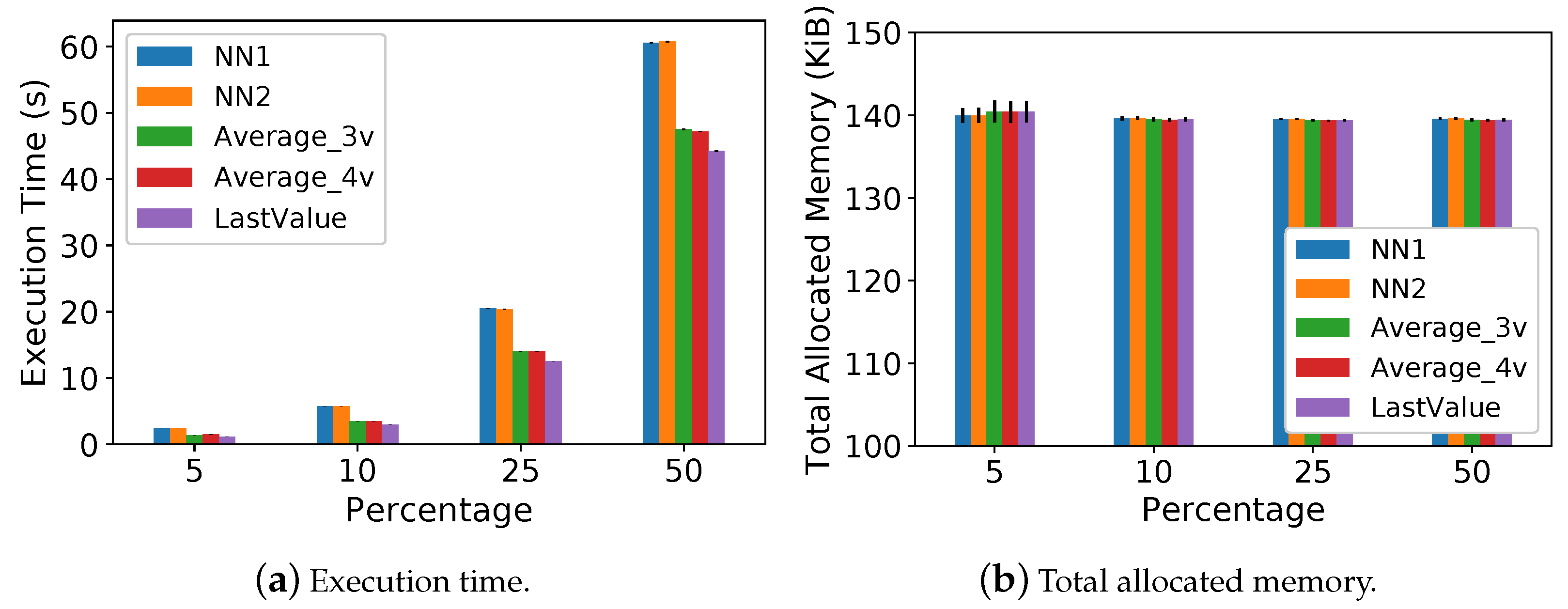
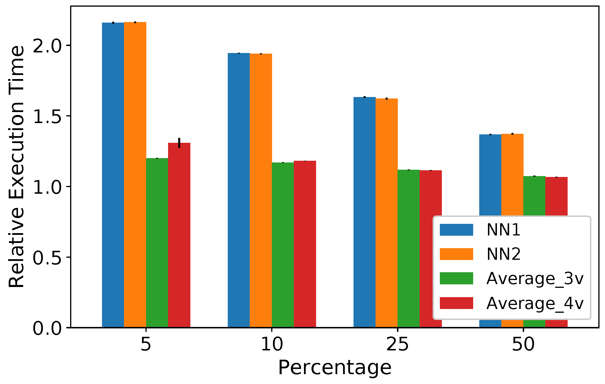
5.2. Execution Time and Memory Usage Analysis

Our mechanism aims to work on IoT gateways, which have scarce computational resources. Therefore, we also need to analyze the implementation’s processing and memory requirements beyond the prediction quality. The training phase usually runs in a Cloud server with more resources. However, verifying whether an IoT gateway can train the models is essential to give more autonomy on the edge for applications that need continuous training. Therefore, the execution time and the memory usage are measured in both training and testing phases. We used the time and tracemalloc Python libraries for the execution time and the allocated memory, respectively. We presented a mean of 50 samples for each missing data percentage with a confidence interval of 95%. The experiments employed a Raspberry Pi 4 Model B with a 1.5 GHz 64-bit quad-core Arm Cortex-A72 CPU and 4 GB of RAM. We chose the Raspberry Pi due to its wide use in the literature of IoT gateways [37,38].

Only the neural network models need training. Thus, we measure the execution time and memory usage to train all attributes in the training phase. In the testing phase, we measure each method’s execution time and memory usage to impute all missing data from the test dataset. In other words, this analysis imputes missing data in a batch. It is important to note that it is a worst-case analysis since only one record is imputed at a time in an online environment. Hence, the execution time and memory usage to impute a single record are much shorter than the following results.

Figure 7 shows the execution time and total memory allocated during the training phase for $NN1$ and $NN2$. Figure 8 shows these same metrics for the testing phase, considering all methods. Figure 7a,b show that, in the training phase, both neural network models take less than 30 s and need less than 4200 KiB of memory. Regarding the testing phase, Figure 8a shows that the execution time increases as the missing data percentage increases for all methods. It is true since more data are imputed as we increase the missing percentage. Figure 8b shows a low memory footprint for all methods with less than 140 KiB of allocation.

The results of Figure 8a show that $LastValue$ is the fastest method in all missing data percentages due to its simplicity. The neural network models are slightly slower than the other methods. For example, they take less than 20 s more than the $LastValue$ for 50% of missing data. However, we imputed missing data in a batch rather than online as a worst-case analysis. Hence, the execution time increase is not prohibitive for the major part of IoT applications.

In an IoT scenario, gateways might have different hardware configurations. Therefore, we take the execution time of the simplest methods (i.e., $LastValue$) as a reference and compare it to the others to verify how slow they are in the testing phase. This comparison allows a more generalized analysis, showing relative values. Figure 9 shows the relative execution time, that is, a method’s execution time over $LastValue$’s execution time. All methods are slower than the $LastValue$ for all percentages, but their worst result occurs when the dataset contains 5% of missing data. Both $NN1$ and $NN2$ are approximately 2.2 times slower than the $LastValue$. For $Average\_3v$ and $Average\_4v$, this difference decreases, and they are approximately 1.2 and 1.3 times slower, respectively. However, as shown in Figure 8a, the absolute values for the execution time are still small.

The results of Figure 8 and Figure 9 show that, although $LastValue$ is faster than the proposed neural networks, these models are still competitive in terms of computational resources. In addition, the high $R^2$ score, low RMSE, and the amount of memory required justify their use, despite the increase in the execution time. Therefore, the results confirm that an IoT gateway can execute both neural network models.

5.3. Neural Network Training Analysis

In Section 5.1 and Section 5.2, both the training and testing datasets have the same missing data percentage. However, in reality, it is not possible to know a priori the missing data percentage that an IoT gateway receives. It means that, after training a model with a certain missing data percentage, one cannot guarantee that the received data have the expected missing data percentage. In this section, using the same methodology as that described in Section 4.2, we trained the neural network models with a fixed missing data percentage, and we tested them in datasets with varying missing data percentages. We aimed to analyze the difference between the missing data percentages in training and testing datasets.

Figure 10 and Figure 11 show, respectively, the $R^2$ scores and RMSE when we train the neural networks considering training datasets with 5% and 50% of missing data for the temperature attribute. We only show this attribute’s results for conciseness since the behavior for the other attributes leads to the same conclusions. The $LastValue$ method does not need any training, but we show its results for comparison purposes. The $Average\_3v$ and $Average\_4v$ also do not need training. However, we omit them since their results were worse than the $LastValue$ in Section 5.1.

The results of Figure 10 show that the neural network models have close $R^2$ scores, regardless of whether the training dataset has 5% or 50% of missing data. Differently from $NN1$, it is possible to note that $NN2$ trained with 5% missing data performed better than when it was trained with 50% missing data. This happened because $NN2$ needs one more input value than $NN1$ (i.e., the measure of the previous day at the same hour). Thus, it has a higher sensibility to missing data on the training dataset. In Figure 11, the RMSE results for the neural networks are smaller than the $LastValue$, and they remain low even when the dataset has 50% of missing data.

In a nutshell, these results show that, despite training the neural networks with a fixed missing data percentage, their performance is still better than the other methods, regardless of the missing data percentage in the test dataset. The occurrence of isolated losses can explain this low sensibility to losses after missing data insertion. Since they are isolated, the training phase is not severely affected. It is an interesting result since a real scenario has small loss bursts, as shown in Section 4.2. Hence, for a real scenario, we expected a low sensibility to losses in our models.

5.4. Case Study—Clustering Application

Although widely used in different fields, some machine learning algorithms did not perform well when they were missing data in the dataset, requiring only complete records. Eliminating the incomplete records may reduce the analysis reliability, which justifies imputing missing data. This subsection presents a case study of an application that uses the DBSCAN [39] clustering algorithm, analyzing how each imputation method affects the algorithm’s outlier detection.

DBSCAN requires two parameters: eps, which specifies the maximum distance that two points must have to be considered neighbors; and min_points, which corresponds to the minimum number of neighbors a point may have to be considered a core point. Hence, all neighbors that are a radius eps apart from the core point belong to the same cluster as that core point [39,40]. The min_points parameter is usually twice the number of the dataset’s attributes [40]. However, for large datasets, with much noise, higher values for min_points may improve the clustering results.

In this experiment, we used two base datasets. For the first set, named $DropTest$, all records that have at least one missing value were eliminated from the set. Hence, all records are complete and have only data measured by sensors. For the second set, named PosInf, instead of eliminating the incomplete records, we used the imputation methods discussed before. Therefore, we create five new sets: $PosInf$-$NN1$, $PosInf$-$NN2$, $PosInf$-$Average\_3v$, $PosInf$-$Average\_4v$, and $PosInf$-$LastValue$. They used, respectively, the imputation methods $NN1$, $NN2$, $Average\_3v$, $Average\_4v$ and $LastValue$.

We ran the DBSCAN algorithm over all six datasets, with different min_points values (i.e., 24, 72, 120, 240, and 720). The eps parameter was calculated using the distance from the record’s k-nearest neighbors [39]. As the $Droptest$ dataset does not have records with predicted values, and it has less data than the other sets, we use it as baseline to choose the eps parameter. We considered $k=\mathtt{min}\_\mathtt{points}$. Therefore, using the $DropTest$ dataset, an eps value was computed for each $k=\mathtt{min}\_\mathtt{point}$ and used in the DBSCAN executions for all datasets with such min_point value.

In this analysis, we aimed to verify whether records with predicted values harm the DBSCAN clustering results and outlier detection. We sought to verify whether:

• After imputing missing data, records previously considered valid become outlier;
• PosInf sets have the same outliers as $DropTest$;
• Any record considered an outlier is no longer an outlier after imputing missing data;
• Records with predicted values are defined as outliers by DBSCAN.

Table 3. The percentage of outliers in common with DropTest (%).

min_points	PosInf- NN1	PosInf- NN2	PosInf- Average_3v	PosInf- Average_4v	PosInf- LastValue
24	93.98	95.83	95.83	97.22	95.37
72	99.52	100.00	99.03	98.55	99.03
120	98.78	99.39	98.78	99.39	98.17
240	100.00	100.00	98.59	100.00	98.59
720	98.92	98.92	94.62	94.62	97.85

shows, in percentage, how many outliers the PosInf datasets have in common with the $DropTest$ dataset, for all tested min_points. For min_points over 24, the PosInf-NN2 dataset is the set with more outliers in common, tying with PosInf-NN1 and PosInf-Average_4v at some min_points. For min_points 24 and 720, the PosInf-Average_4v dataset has less outliers than $DropTest$, and that is the reason for which it shows a low intersection with it. The same occurs in the PosInf-Average_3v dataset, when min_points = 720. In these cases, some outlier records are no longer considered outliers when the records with imputed data are inserted. Therefore, depending on the imputation method used, records previously identified as outliers might become valid in DBSCAN. It happens since the inclusion of records with imputed data can decrease the distance between a record and a core point.

Table 4. DBSCAN results’ comparison when min_points = 72. Adapted from [23].

Dataset	Total	Outliers	New Outliers
DropTest	16,777	207	-
PosInf-NN1	17,544	217	11
PosInf-NN2	17,544	215	8
PosInf-Average_3v	17,544	219	14
PosInf-Average_4v	17,544	208	4
PosInf-LastValue	17,544	222	17

shows the DBSCAN results for all datasets when min_points = 72. This shows the number of records in each dataset and the number of outliers detected by DBSCAN. In addition, the “new outliers” column shows how many records are not considered outliers in the $DropTest$, but are outliers in the $PosInf$ sets. Manual analysis indicates that all “New outliers” are records with predicted data. Hence, they do not exist in the $DropTest$ dataset. Therefore, imputing missing values does not make a valid record into an outlier. In addition, some methods insert more outliers than others.

The PosInf datasets have 767 records with imputed values. Our subsequent analysis is to verify how many of those are identified as outliers by DBSCAN, as we vary the min_points.

Table 5. Percentage of outliers identified in the imputed records (%). Adapted from [23].

min_points	PosInf- NN1	PosInf- NN2	PosInf- Average_3v	PosInf- Average_4v	PosInf- LastValue
24	2.09	1.30	1.96	0.52	2.22
72	1.43	1.04	1.83	0.52	2.22
120	1.04	0.78	1.43	0.26	1.96
240	0.78	0.65	1.43	0.13	1.69
720	0.26	0.26	0.00	0.00	0.65

shows the outliers’ percentage in each PosInf dataset. It is possible to notice that the percentage of records identified as outliers is less than 2.2% for all cases. In addition, the larger the min_points, the smaller the percentage of outliers inserted by the methods. It happens because some records can become core points and thus bring previous outliers closer together. As defined before, the Average_3v and Average_4v methods compute the average of 3 or 4 values of the dataset, respectively. Therefore, unless these input values are already outliers, the predicted value is probably in the range of valid values. This behavior can be noticed in the PosInf-Average_4v, which is the set with fewer outliers inserted after the imputation of missing data. However, considering the PosInf-Average_3v dataset, we can note that the Average_3v method inserted more outliers than PosInf-Average_4v. This behavior is in line with the $R^2$ and $RMSE$ results, in which this method performed worse than Average_4v.

In this section, the DBSCAN algorithm is an example of an application that requires that all records are complete. The results confirm that the missing data imputation methods provide good results without distorting the DBSCAN results. The neural network models $NN1$ and $NN2$ insert fewer outliers than the $LastValue$ method. The PosInf-Average_4v dataset has the lowest incidence of new outliers. However, this was expected given the nature of such a method. Despite this fact, the previous results of $R^2$ and RMSE show that the neural networks performed better than Average_4v.

6. Discussion

Table 6. Prediction quality performance summary.

Method	${\mathit{R}}^2$	RMSE	Produce Few Outliers?
NN1
NN2
Average_3v
Average_4v
LastValue

summarizes the findings of this work for prediction quality, indicating whether a method has good results for a given metric. This table indicates the best overall performance of our neural network models.

This work shows that it is possible to use simple methods to impute missing data in IoT gateways. This article extends our previous work [23] that presents preliminary results showing the performance of the proposed methods. Although our former paper already showed that $NN1$ and $NN2$ outperformed $LastValue$, it still lacked a more detailed analysis which we addressed in this work. Regarding the results, we discuss next the main improvements compared to [23]:

• Analysis of $\mathit{Average}\_\mathbf{3}\mathit{v}$ and $\mathit{Average}\_\mathbf{4}\mathit{v}$ methods. These methods have the same input data as the neural networks, however, the estimated value is the average of the inputs. Our goal in adding these methods is to verify whether it is indispensable to train a neural network or if a simple average of the same input data already provides good predictions. Our results indicate that $\mathit{NN}\mathbf{1}$ and $\mathit{NN}\mathbf{2}$ outperforms $\mathit{Average}\_\mathbf{3}\mathbf{v}$ and $\mathit{Average}\_\mathbf{4}\mathit{v}$, thus justifying the use of neural networks;
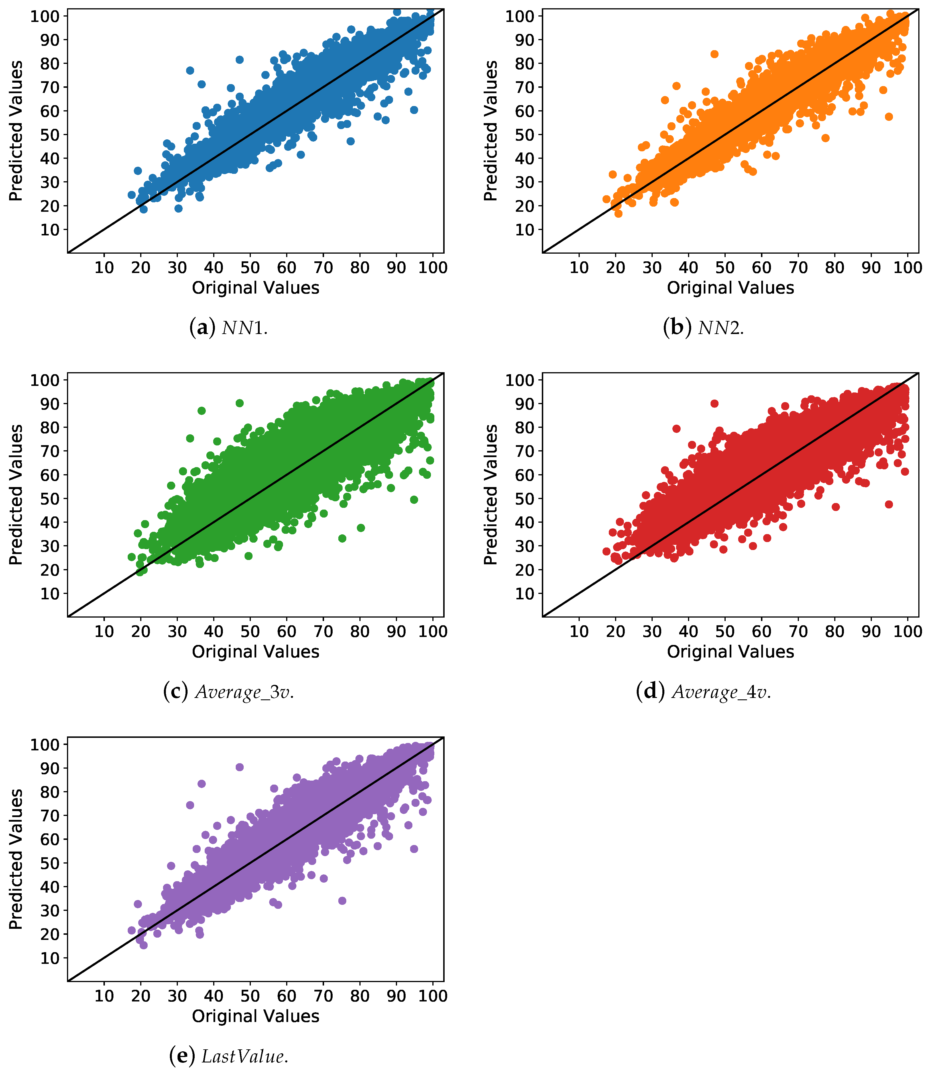
• Analysis comparing the original values with the predicted ones for all methods, as shown in Figure 6. Our idea is to analyze the results from another perspective, to add more consistency to our findings. Hence, this new analysis allows the graphical visualization of our performance improvements. This analysis has shown that $\mathit{NN}\mathbf{1}$ and $\mathit{NN}\mathbf{2}$ present predicted values closer to the original ones than the other methods.
• Analysis summarizing our main findings in Table 6. This table highlights the importance of $\mathit{NN}\mathbf{1}$ and $\mathit{NN}\mathbf{2}$, showing that these methods present the best prediction performance and produce few outliers in a clustering application.

It is important to notice that, in this work, we entirely redesigned our previous work to clarify our motivation, to present additional related work, and to provide a more detailed discussion.

7. Conclusions

Collected data from IoT systems might have missing data due to various reasons such as network problems, damaged sensors, or security attacks. To provide a more efficient analysis and thus reliable services, we must address the missing data problem. Traditionally, a Cloud server performs this task. However, some applications require real-time response, which can be challenging to achieve using a cloud server due to the amount of data, the networking traffic, and the delay. Furthermore, we propose a simple mechanism to run in IoT gateways that imputes missing data using regression models based on neural networks. Our goal is to verify whether these simple models perform well in IoT gateways, which usually have scarce resources.

We used actual weather data from Rio de Janeiro to validate our models. The results show that the neural network models have a high $R^2$ score and low RMSE for different missing data percentages, performing better than other simple methods. In addition, our models present a short execution time and need less than 140 KiB of memory, which allows them to be used in IoT environments. We also showed that our models present good results even when we fixed the missing data percentage in the training set and varied the missing data percentages in the test set. With only 50% of complete records available for training in our experiments, the neural network models still performed well.

This work also presented a case study that used a clustering algorithm to analyze the neural network models as imputation methods. The algorithm’s results show that only a small percentage of the records with imputed values are considered outliers. Therefore, the imputation methods can deal with missing data without distorting the application’s results. Finally, using simple imputation methods, we confirm that an application can use all data received by sensors without eliminating the incomplete records.

In this work, we inserted the missing data in the dataset using uniform distribution to study the impact of the isolated losses. In future work, other patterns of missing data insertion may be used. For example, we could analyze how the neural network models performed when the missing data occur in large-sized bursts. Another extension of this work would be to use data with more variability and dynamism to verify whether the models’ performance remains high. Finally, another line for future work is to evaluate the behavior of the periodic updating of the models in an online learning scenario.

References

1. Correia, L.; Fuentes, D.; Ribeiro, J.; Costa, N.; Reis, A.; Rabadão, C.; Barroso, J.; Pereira, A. Usability of Smartbands by the Elderly Population in the Context of Ambient Assisted Living Applications. Electronics 2021, 10, 1617. [Google Scholar] [CrossRef]
2. Santos, S.C.; Firmino, R.M.; Mattos, D.M.; Medeiros, D.S. An IoT rainfall monitoring application based on wireless communication technologies. In Proceedings of the 4th Conference on Cloud and Internet of Things (CIoT), Niterói, Brazil, 7–9 October 2020; pp. 53–56. [Google Scholar]
3. Siddique, K.; Akhtar, Z.; Lee, H.g.; Kim, W.; Kim, Y. Toward bulk synchronous parallel-based machine learning techniques for anomaly detection in high-speed big data networks. Symmetry 2017, 9, 197. [Google Scholar] [CrossRef] [Green Version]
4. Kim, D.Y.; Jeong, Y.S.; Kim, S. Data-filtering system to avoid total data distortion in IoT networking. Symmetry 2017, 9, 16. [Google Scholar] [CrossRef] [Green Version]
5. Gantert, L.; Sammarco, M.; Detyniecki, M.; Campista, M.E.M. A supervised approach for corrective maintenance using spectral features from industrial sounds. In Proceedings of the IEEE 7th World Forum on Internet of Things (WF-IoT), New Orleans, LO, USA, 14 June–31 July 2021. [Google Scholar]
6. Cruz, P.; Silva, F.F.; Pacheco, R.G.; Couto, R.S.; Velloso, P.B.; Campista, M.E.M.; Costa, L.H.M.K. SensingBus: Using Bus Lines and Fog Computing for Smart Sensing the City. IEEE Cloud Comput. 2018, 5, 58–69. [Google Scholar] [CrossRef]
7. Schmitt, P.; Mandel, J.; Guedj, M. A comparison of six methods for missing data imputation. J. Biom. Biostat. 2015, 6, 1–6. [Google Scholar]
8. Yan, X.; Xiong, W.; Hu, L.; Wang, F.; Zhao, K. Missing value imputation based on gaussian mixture model for the internet of things. Math. Probl. Eng. 2015, 2015, 548605. [Google Scholar] [CrossRef]
9. Liu, Y.; Dillon, T.; Yu, W.; Rahayu, W.; Mostafa, F. Missing value imputation for Industrial IoT sensor data with large gaps. IEEE Internet Things J. 2020, 7, 6855–6867. [Google Scholar] [CrossRef]
10. Al-Milli, N.; Almobaideen, W. Hybrid neural network to impute missing data for IoT applications. In Proceedings of the IEEE Jordan International Joint Conference on Electrical Engineering and Information Technology (JEEIT), Amman, Jordan, 9–11 April 2019. [Google Scholar]
11. Purohit, L.; Kumar, S. Web services in the internet of things and smart cities: A case study on classification techniques. IEEE Consum. Electron. Mag. 2019, 8, 39–43. [Google Scholar] [CrossRef]
12. Guastella, D.A.; Marcillaud, G.; Valenti, C. Edge-Based Missing Data Imputation in Large-Scale Environments. Information 2021, 12, 195. [Google Scholar] [CrossRef]
13. Pan, J.; Yang, Z. Cybersecurity Challenges and Opportunities in the New “Edge Computing+IoT” World. In Proceedings of the 2018 ACM International Workshop on Security in Software Defined Networks & Network Function Virtualization, Tempe, AZ, USA, 21 March 2018. [Google Scholar]
14. Fekade, B.; Maksymyuk, T.; Kyryk, M.; Jo, M. Probabilistic recovery of incomplete sensed data in IoT. IEEE Internet Things J. 2017, 5, 2282–2292. [Google Scholar] [CrossRef]
15. Li, D.; Deogun, J.; Spaulding, W.; Shuart, B. Towards missing data imputation: A study of fuzzy k-means clustering method. In International Conference on Rough Sets and Current Trends in Computing; Springer: Berlin/Heidelberg, Germany, 2004. [Google Scholar]
16. Mary, I.P.S.; Arockiam, L. Imputing the missing data in IoT based on the spatial and temporal correlation. In Proceedings of the IEEE International Conference on Current Trends in Advanced Computing (ICCTAC), Bangalore, India, 2–3 March 2017. [Google Scholar]
17. Guzel, M.; Kok, I.; Akay, D.; Ozdemir, S. ANFIS and Deep Learning based missing sensor data prediction in IoT. Concurr. Comput. Pract. Exp. 2020, 32, e5400. [Google Scholar] [CrossRef]
18. Nikfalazar, S.; Yeh, C.H.; Bedingfield, S.; Khorshidi, H.A. Missing data imputation using decision trees and fuzzy clustering with iterative learning. Knowl. Inf. Syst. 2020, 62, 2419–2437. [Google Scholar] [CrossRef]
19. Kök, İ.; Özdemir, S. DeepMDP: A Novel Deep-Learning-Based Missing Data Prediction Protocol for IoT. IEEE Internet Things J. 2020, 8, 232–243. [Google Scholar] [CrossRef]
20. Zhang, Y.F.; Thorburn, P.J.; Xiang, W.; Fitch, P. SSIM—A deep learning approach for recovering missing time series sensor data. IEEE Internet Things J. 2019, 6, 6618–6628. [Google Scholar] [CrossRef]
21. Turabieh, H.; Salem, A.A.; Abu-El-Rub, N. Dynamic L-RNN recovery of missing data in IoMT applications. Future Gener. Comput. Syst. 2018, 89, 575–583. [Google Scholar] [CrossRef]
22. Izonin, I.; Kryvinska, N.; Tkachenko, R.; Zub, K. An approach towards missing data recovery within IoT smart system. Procedia Comput. Sci. 2019, 155, 11–18. [Google Scholar] [CrossRef]
23. França, C.M.; Couto, R.S.; Velloso, P.B. Data imputation on IoT gateways using machine learning. In Proceedings of the 19th Mediterranean Communication and Computer Networking Conference (MedComNet), Ibiza, Spain, 15–17 June 2021. [Google Scholar]
24. Chong, A.; Lam, K.P.; Xu, W.; Karaguzel, O.T.; Mo, Y. Imputation of missing values in building sensor data. Proc. Simbuild 2016, 6, 407–414. [Google Scholar]
25. Troyanskaya, O.; Cantor, M.; Sherlock, G.; Brown, P.; Hastie, T.; Tibshirani, R.; Botstein, D.; Altman, R.B. Missing value estimation methods for DNA microarrays. Bioinformatics 2001, 17, 520–525. [Google Scholar] [CrossRef] [PubMed] [Green Version]
26. Honghai, F.; Guoshun, C.; Cheng, Y.; Bingru, Y.; Yumei, C. A SVM regression based approach to filling in missing values. In International Conference on Knowledge-Based and Intelligent Information and Engineering Systems; Springer: Berlin/Heidelberg, Germany, 2005. [Google Scholar]
27. Azimi, I.; Pahikkala, T.; Rahmani, A.M.; Niela-Vilén, H.; Axelin, A.; Liljeberg, P. Missing data resilient decision-making for healthcare IoT through personalization: A case study on maternal health. Future Gener. Comput. Syst. 2019, 96, 297–308. [Google Scholar] [CrossRef]
28. Rubin, D.B. Inference and missing data. Biometrika 1976, 63, 581–592. [Google Scholar] [CrossRef]
29. González-Vidal, A.; Rathore, P.; Rao, A.S.; Mendoza-Bernal, J.; Palaniswami, M.; Skarmeta-Gómez, A.F. Missing Data Imputation with Bayesian Maximum Entropy for Internet of Things Applications. IEEE Internet Things J. 2020. [Google Scholar] [CrossRef]
30. Izonin, I.; Kryvinska, N.; Vitynskyi, P.; Tkachenko, R.; Zub, K. GRNN approach towards missing data recovery between IoT systems. In International Conference on Intelligent Networking and Collaborative Systems; Springer: Berlin/Heidelberg, Germany, 2019; pp. 445–453. [Google Scholar]
31. Drucker, H. Improving regressors using boosting techniques. In ICML; Citeseer: Nashville, TN, USA, 1997; Volume 97, pp. 107–115. [Google Scholar]
32. Smola, A.J.; Schölkopf, B. A tutorial on support vector regression. Stat. Comput. 2004, 14, 199–222. [Google Scholar] [CrossRef] [Green Version]
33. Siami-Namini, S.; Tavakoli, N.; Namin, A.S. A comparison of ARIMA and LSTM in forecasting time series. In Proceedings of the 2018 17th IEEE International Conference on Machine Learning and Applications (ICMLA), Orlando, FL, USA, 17–20 December 2018; pp. 1394–1401. [Google Scholar]
34. Wang, C.; Shakhovska, N.; Sachenko, A.; Komar, M. A New Approach for Missing Data Imputation in Big Data Interface. Inf. Technol. Control 2020, 49, 541–555. [Google Scholar] [CrossRef]
35. Gardner, M.W.; Dorling, S. Artificial neural networks (the multilayer perceptron)—A review of applications in the atmospheric sciences. Atmos. Environ. 1998, 32, 2627–2636. [Google Scholar] [CrossRef]
36. Pedregosa, F.; Varoquaux, G.; Gramfort, A.; Michel, V.; Thirion, B.; Grisel, O.; Blondel, M.; Prettenhofer, P.; Weiss, R.; Dubourg, V.; et al. Scikit-learn: Machine Learning in Python. J. Mach. Learn. Res. 2011, 12, 2825–2830. [Google Scholar]
37. Raza, S.M.; Jeong, J.; Kim, M.; Kang, B.; Choo, H. Empirical Performance and Energy Consumption Evaluation of Container Solutions on Resource Constrained IoT Gateways. Sensors 2021, 21, 1378. [Google Scholar] [CrossRef]
38. Glória, A.; Cercas, F.; Souto, N. Design and implementation of an IoT gateway to create smart environments. Procedia Comput. Sci. 2017, 109, 568–575. [Google Scholar] [CrossRef]
39. Ester, M.; Kriegel, H.P.; Sander, J.; Xu, X. A density-based algorithm for discovering clusters in large spatial databases with noise. KDD 1996, 96, 226–231. [Google Scholar]
40. Schubert, E.; Sander, J.; Ester, M.; Kriegel, H.P.; Xu, X. DBSCAN revisited, revisited: why and how you should (still) use DBSCAN. ACM Trans. Database Syst. (TODS) 2017, 42, 1–21. [Google Scholar] [CrossRef]
Figure 1. Missing data imputation mechanism. Adapted from [23]. This figure uses icons made by Freepik, from www.flaticon.com (accessed on 29 September 2021).
Information 12 00425 g001
Figure 2. Percentage of missing data of São Cristóvão station (%) [23].
Information 12 00425 g002
Figure 3. Cumulative probability of the burst size using data from 2015 to 2016.
Information 12 00425 g003
Figure 4. R 2 score for atmospheric pressure, temperature, and humidity attributes.
Information 12 00425 g004
Figure 5. RMSE for atmospheric pressure, temperature, and humidity attributes.
Information 12 00425 g005
Figure 6. Predicted x original for relative humidity.
Information 12 00425 g006
Figure 7. Execution time and memory footprint on the training phase.
Information 12 00425 g007
Figure 8. Execution time and memory footprint on the testing phase.
Information 12 00425 g008
Figure 9. Relative execution time on the testing phase.
Information 12 00425 g009
Figure 10. R 2 score for temperature using a fixed missing data percentage on the training dataset.
Information 12 00425 g010
Figure 11. RMSE for temperature using a fixed missing data percentage on the training dataset.
Information 12 00425 g011