Abstract
The problem of forged images has become a global phenomenon that is spreading mainly through social media. New technologies have provided both the means and the support for this phenomenon, but they are also enabling a targeted response to overcome it. Deep convolution learning algorithms are one such solution. These have been shown to be highly effective in dealing with image forgery derived from generative adversarial networks (GANs). In this type of algorithm, the image is altered such that it appears identical to the original image and is nearly undetectable to the unaided human eye as a forgery. The present paper investigates copy-move forgery detection using a fusion processing model comprising a deep convolutional model and an adversarial model. Four datasets are used. Our results indicate a significantly high detection accuracy performance (~95%) exhibited by the deep learning CNN and discriminator forgery detectors. Consequently, an end-to-end trainable deep neural network approach to forgery detection appears to be the optimal strategy. The network is developed based on two-branch architecture and a fusion module. The two branches are used to localize and identify copy-move forgery regions through CNN and GAN.
1. Introduction
The hot topic known as “fake news” is becoming increasingly widespread across social media, which for many people has become their primary news source. Fake news is information that has been altered to represent a specific agenda. To support the production of fake news, images that have been tampered with are often presented with the associated reports. Fake news production has been enabled in recent years because of two main reasons: first, cost reductions of the required image-producing technology (e.g., cell phones and digital cameras); and second, the widespread accessibility of image-editing software from open-source tools and apps. Anyone with a cell phone or digital camera who has online access to the necessary software can now alter images easily and cheaply, for whatever purpose. At the same time, online access enables the images to be sent across a virtually limitless number of platforms, where they can be further altered through dedicated imagery software (e.g., Photoshop) using tools such as splicing, painting, or copy-move forgery.
Considering how easy it is to create fake images as part of a fake news report, there is a critical need for detection methods that can keep up with the latest technology in fraud production. The integrity of an image can be validated through one or more strategies, either alone or in combination, which test an image for authenticity [1,2,3]. A popular strategy is copy-move image forgery, which involves copying or cloning an image patch into an identical image. The patches to be copied or clones can be either irregular or in regular form. Copy-move image forgery is increasing in popularity due in large part to its ease of use. Furthermore, because the copied or cloned patch has its source in the original image, photometric characteristics between the original and the forgery are essentially the same, making it that much more difficult for the fake to be detected.
Since its recent development at around the turn of the present century [4,5], the primary purpose for copy-move forgery detection (CMFD) has been determining if the imaging probe in question (otherwise known as the query) features any areas that are cloned, and whether this cloning has been performed with malicious intent. The three main types of copy-move forgeries are plain, affine, and complex [6]. The earliest CMFD investigations dealt mostly with plain cloning. Interestingly, in a previous study [7], the researchers found that human judgment outsmarted machine learning regarding computer-generated forgeries. This could be caused by the current lack of photorealism found in most computer graphics tools.
In response to this flaw, various researchers suggested alternative approaches to analyzing digital imagery. Examples include, statistics extracted from wavelet decomposition [8] and statistics extracted from residual images [9]. Researchers have focused on noise type and level based on recording devices [10], chromatic aberrations [11], or demos icing filters [12]. Additionally, some researchers have looked at color distribution differences [13], whereas others examined the statistical properties found in local edge patches [14]. Currently, deep learning is being successfully applied in a range of applications, as demonstrated in previous work [7,15,16].
Given the increasing difficulty to distinguish between photographic and computer-generated forgeries, the need to develop equally sophisticated detection modes is becoming more urgent [17]. The latest incarnations of computer-vision-based image forgeries show a significantly higher degree of photorealism than was previously exhibited [18,19,20,21,22,23]. Especially compelling is image copy-move forgery (CMF), which changes the features of one image by digitally translating one scene as another [24]. CMF is further enabled by generative adversarial networks (GANs), whose sole purpose is to produce “knock-off” images that are virtually identical to the original ones.
The present work investigates the state-of-the-art of CMF and proposes a suitable algorithm that can detect and localize image copy-move forgery. The approach is derived from a new strategy for deep neural architecture that detects CMFs by applying generative adversarial networks. The proposed algorithm assumes that because no forged images will be accessible for training purposes, feature representations for pristine images are then made available solely on the basis of training tasks. Therefore, a one-class support vector machine (SVM) has been trained in alignment with the characteristics of the images in order to gauge distribution. Any forged images can then be determined according to anomalies found in the distribution patterns. The classifier will determine the image differently based on its pattern’s distribution.
2. Related Works
According to feature extraction and matching schemes, copy-move detection strategies are categorized as one of three different types: block-based or patch methods, keypoint methods, and irregular region-based methods. In the first approach, block-based methods have applied chroma features in some research studies [25,26], as well as in PCA features [27], blur moments [28], DCT [29], and Zernike moments [30]. However, this is a relatively computationally expensive approach compared to the other two. The second approach category, keypoint-based methods, includes triangles [31], ORB [32], SURF [32,33,34], and SIFT [35,36,37]. Keypoint approaches are known to be generally fast, but they can fail if source S and destination D show as homogeneous. Meanwhile, the third category deals with strategies related to irregular region-based methods [29,38], and has been shown to be somewhat efficient, though occasionally resulting in false positives [39,40,41,42].
Datasets can be enhanced using a group of GAN derivative models. These models also have the additional use of classifying images that show a promising result [43]. Many examples have proven their use in solving problems with a low number of samples, performing the aforementioned tasks and improving the accuracy of the trainer in many cases, such as in the detection of image forgery [44,45]. The general process of GAN is simple—a distribution model is captured and used to create a new data sample. A real distribution model is captured and then regenerated by the generator to produce a new data sample. A discriminator then determines whether the input data sample is real or generated, while the discriminator works with the generator by challenging and checking each other, optimizing their parameters. In a specific example [46], a GAN-based deep learning image classifier was used to develop a deep forgery discriminator. Its purpose was to detect fake faces in public, and it did that with 94.7% accuracy. Because the classic techniques cannot detect the forgery in the forged images generated by GANs, using a deep learning forgery discriminator is highly recommended. CNN, on the other hand, takes a step ahead in the same field for image CMF localization based on feature similarity detection [47]. Their features are extracted from an image by convolving the image using a chosen filter, such as a Kernel filter or Gabor filter, or combining them to generate a feature map of the same input image [48]. Measuring the similarity can be done by applying a cosine similarity function [49].
By observing a few copy-move forged images, it was evident that locating the forged areas by human visual detection is difficult, and in some cases, impossible. Thus, CNN is the perfect deep learning model for this job, and it is used jointly with GAN to ensure the performance of the proposed model. Therefore, based on the above, the use of deep learning DNN and GAN models to detect and localize digital image forgery is a newly active trend in this era.
The latest research on image forgery detection focuses on deep neural networks (DNNs). In one study [50], DNN was applied for extraction of features in CMF, while in another study [51], altered areas of the image were detected using a DNN-based patch classifier. The researchers in [52] looked for a way to detect localization and splicing using a DNN solution, and [53] explored how DNN can be used in detecting images that have been doctored, as well as detecting the fake generated images, as in [54]. In general, GAN-based methods provide the most optimal results in image forgery detection, with the majority of the applications using numerous paired images from both domains to train the networks. In instances where no image pairs have been made available for the training process, an alternative method can be used to continue in the GAN approach.
The adversarial training paradigm features two main components: the generator (i.e., the image-to-image network) and the discriminator (i.e., the support network). Within the paradigm, the generator’s training revolves around learning to deceive the discriminator, while the discriminator is trained to detect real images from forged ones [55,56,57]. In a previous study [23], Zhu et al. devised a method for automatically pairing images, thus, overcoming the shortage in genuine image pairs. For a baseline, Zhu and colleagues [23] employed a discriminator in the GAN. Nonetheless, there are a few methods where explicit delineation of a probability distribution is not performed. In these cases, generative machines are trained to obtain samples within a specific distribution source. The main benefit of using this technique is being able to design the machines for the desired training task. Also, the previous methods in the above related works are used to detect the image forgery in general, and most of them perform well in detecting that type of forgery. This study, however, focuses specifically on copy-move forgery detection. Nonetheless, all of the mentioned related works have at least two out of the three following problems: first, having low accuracy rate; second, being computationally expensive; third, being unable to distinguish between the source and the target forger area. On the other hand, the proposed algorithm in this study employed GAN and CNN in parallel to detect the copy-move forgery. It performed well and became able to express the source image patch versus the forged one with compromised operation cost.
3. Proposed Copy-Move Forgery Detection Strategy
3.1. GANs Create Forged Images
Advances in technology are enabling GANs to create forged images that fool even the most sophisticated detectors [58]. It is important to note that the primary aim of generative adversarial networks is to form images that cannot be distinguished from the original source image. Figure 1 below depicts image forgery translation enabled by GANs.
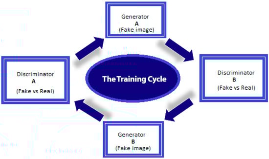
Figure 1.
The GAN training cycle for fake image translation (i.e., fake image creation based on a real image).
As can be seen, generator has been employed to transform input image A from a domain to output domain . Next, generator is used to map image B back to the domain (the original domain). In doing so, two more cycle consistency losses are added to the typical adversarial losses borne by the discriminators, thus, obtaining A = ((A)) and enabling the two images to be paired. Extremely sophisticated editing tools are required to change an image’s context. These tools must be able to alter images while retaining the original source’s perspective, shadowing, and so on. Those without forgery detection training would likely be unable to distinguish the original from an image forged using this method, which means that it is a good candidate for developing supporting materials for fake news reports.
3.1.1. GAN Tasks
GAN tasks are as follows: (1) Load dataset; (2) build discriminator network; (3) build generator network; (4) generate a sample image; (5) training difficulties; (7) closing thoughts. The GAN network branch is presented in Figure 2.
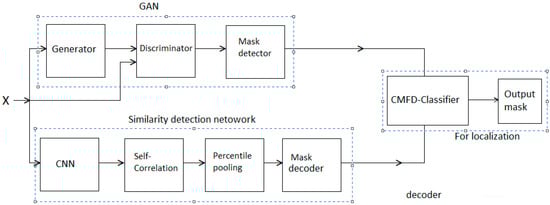
Figure 2.
Layout of the proposed model.
3.1.2. GAN Processing Steps
In our proposed GAN network, we consider three main steps: (1) In the first step, the generator creates an image from random noise input. (2) The image is then presented to the discriminator, together with several images derived from the same dataset. (3) After the discriminator is presented with the real and forged images, it provides probabilities in the form of a number between 0 and 1, inclusive. Here, 0 indicates a forged image and 1 indicates a high likelihood for authenticity. Note that the discriminator should be pretrained prior to the generator, as this creates a clearer gradient. It is important to retain constant values for both the discriminator and generator when training their opposites (i.e., the values for the discriminator are steady when training the generator, and vice versa). Holding the values constant enables the networks to have a greater understanding of the gradient, which is the source of its learning. However, because GANs have been developed as a type of game played between opposing networks, maintaining their balance can be challenging. Unfortunately, learning is difficult for GANs if the discriminator or generator is too adept, because GANs generally require a lengthy training period. So, for instance, a GAN could take several hours for a single GPU, while for a single CPU, a GAN could require several days [59].
3.1.3. Support Vector Machines
Recently, there has been a decline in reliance on support vector machines (SVM) [60], particularly kernel SVMs, as they require real-valued vectors. Users and researchers are instead turning to machine learning systems as end-to-end learning models. In general, deep learning architectures usually source the classifier function and feature representations solely from training examples, but we employed a linear SVM toward the end of every deep convolutional neural network branch. We then trained them jointly by applying a backpropagation algorithm and stochastic gradient descent (input→→convNet→→SVM→→output). Note that the linear SVM has been given a linear activation function (similar to a regression function), with the hinge loss replacing the loss function, as follows:
where and . It is also possible to use a stochastic sub-gradient descent rather than an SGD, given that the hinge-loss cannot be differentiable. The training, thus, occurs end-to-end, with the hinge-loss error signal guiding the convNet and SVM weight learning. Furthermore, because hinge-loss causes the linear units to connect with learning maximum margin hyperplanes, linear SVMs are the outcome.
As an example, a linear unit is connected by the hinge-loss, resulting in a single linear SVM + a trained convNet as feature detection after training. In this setup, the SVM is designed to learn the final splitting hyperplane and the convNet is designed to learn the hierarchical features. Following the training procedure, a Heaviside step function can then be applied against the linear SVM output to obtain a binary output. The idea of using SVM in forgery detection is based on capturing the difference before knowing for certain that the patch is forged, which requires the use of a one-class SVM. This entity, which has been trained using feature vector that is extracted from input images, quickly learns pristine feature distribution versus the forgery feature distribution. Next, it outputs a soft value that indicates the degree of possibility that the feature vector is pristine or forged. The soft mask is then defined as a matrix that has identical dimensions to the image, with every entry having a soft SVM output corresponding to image patches at identical positions. A final detection binary mask can be obtained by employing the soft mask for thresholding. More details will be provided in the following section.
A summary of the copy-move forgery detection (CMFD) strategies employed in the present work is given in this section. Figure 2 illustrates the pipeline for the proposed technique. As shown in the figure, our proposed approach employs two distinct networks for forgery detection. One of the networks is GAN-based and detects any symptom of forgery, while the other locates any similarities existing in the image. As a joint network, the proposed method then locates any copy-move forgery found in the imagery target, demarcating the original source from the copy-moved region of the image. In CMFD-related tasks, the input data proceed through the two networks, GAN and CNN, and are then assigned to a linear classifier based on the proposed model selection. The CNN, in general, maintains feature extraction and ability to generate features versus strong discrimination skills, therefore the proposed model is used for data generation, feature extraction, data discrimination, and data classification.
3.2. CNN for Matching or Detecting Similar Patches
A critical issue in copy-move forgery detection is in images containing features that are nearly identical, although matching visual content for the same or diverse images can be done [4]. The important element in matching methods is how much rigidity ensues after the correspondences are computed. In most instances, matching size options are relatively manageable, but they can also be extreme, in which case the problem is unconstrained. Recently, some methods have been developed that can detect matching objects throughout an image and across several different viewpoints [5,6], but improvements can still be made [21]. Such improvements could include involving convolutional deep neural networks, as these networks are relatively easily trainable end-to-end. For local feature representations, researchers have used deep learning in different copy-move forgery detection stages, such as metric learning, descriptor, and detector stages.
Based on preceding research inquiries, the present work proposes employing deep convolutional neural networks (CNNs) to deal with learning automatic detection in similar feature presentation [22]. CNNs are especially valuable for learning decision features adaptively when working from large data sets [23]. In the present study, the proposed model will learn a number of attributes, such as what are considered good features, how to capture similar pixels across different scales, and finding possible similarities between patches. The proposed model is then evaluated qualitatively and quantitatively, showing its ability to discern and match similar patches across multiple scales. The primary contribution of this work is developing a learning algorithm that can detect copy-move features according to similarities found in detected features within an image frame.
3.2.1. Similarity-Matching Tasks
In similarity-matching tasks, similarities are computed by employing a multi-layer CNN that deconstructs the targeted patches into sub-patches. Under this setup, different scales can be applied and repetitive textures can be used. Local similarities are computed in every individual layer by starting with the assumption that the feasible rigid deformations comprise only a limited set. Detection of the matching features is propagated throughout the sub-patch hierarchy, with the incorrect detections being discarded during the process [6].
As can be seen in Figure 2, the architecture resembles a traditional computer vision pipeline, except for the application of differentiable modules. The addition of these modules enables end-to-end training to occur in the localization tasks, as well as in the main target task of CMFD. The similarity detection network moves all of the images (pristine and forged) through the convolutional layers, and in the process extracting feature maps by employing CNN. This procedure continues through dense local descriptors and percentile pooling to feature maps, and then, using the mask decoder feature, on to the original image size. At this stage, similar feature maps are matched as a tentative correspondence map using binary classifiers. Further details will be provided in the training section below.
3.2.2. Feature Extraction
Traditional CNN architecture is employed for the pipeline’s initial step of feature extraction. In this stage, a CNN that does not have fully connected layers develops a feature map from an input image (). This can also be expressed as a dense spatial grid from d-dimensional local descriptors. In a previous study [39], researchers applied more or less the same interpretation for instance retrieval, showing that CNN-based descriptors had significant discriminative power. Therefore, as feature extraction in the present work, the VGG-16 network will be employed.
This setup features four layers (16 convolutional layers) and conducts 3 × 33\Times 33 × 3 convolutions and 2 × 22\times 22 × 2 pooling throughout the extraction process. Note that this strategy is presently the most popular for image feature extraction.
In employing the technique, however, we decided to modify the terms slightly by cropping the pool4 layer (in front of the ReLU unit) prior to applying per-feature L2 normalization. A pretrained model was used to perform image analyses and classification. Figure 2 illustrates the duplication of the feature extraction network, showing how it is organized as a series configuration. In this arrangement, the input images move along the network path [27,38]. The aim of conducting feature extraction is mainly to boost the learned model’s accuracy through the extraction of the most critical features and the removal of redundancies and noise [30]. Note that in general, feature extraction focuses on extracting useful information out of raw pixel values; the information is considered “useful” if it can distinguish among various categories. Following successful feature extraction, the images and related labels are then used to train a classification module that will be used in measuring distances toward the detection of similarities.
3.2.3. Feature Extraction Problems
Accurate and efficient feature extraction of input data is crucially significant in machine learning. In feature extraction, input data are transformed into feature vectors, which in turn become inputs in learning algorithms. To address the many issues that have arisen over the years in pursuit of optimal feature extraction, researchers have developed a number of techniques, ranging from feature selection to dimensionality reduction to manifold and representation learning [33]. The most promising solution appears to be incorporating CNNs in the VGG16 approach. In this architecture, multiple 3 × 3 kernel-sized filters are used in succession. Multiple stacked small-size kernels function more optimally than large-size ones, as multiple non-linear layers add more depth to the network, allowing for more complex learning and reduced costs. The extraction of relevant features can be done effectively even with a simple approach, and such an approach need not be complex or large to be effective [34].
4. Proposed Algorithm Overview
The present study proposes the construction of a copy-move forgery detection algorithm that features two deep neural networks—a GAN network and a custom CNN-based one. The details of the proposed network are as follows. The GAN network contains both the generator and the discriminator. It will be built first, followed by the custom CNN. The third step in the construction involves merging the two output networks to create a merging network branch. In this section, we will illustrate these networks with more related details.
4.1. Discriminator Network
Constructing the discriminator network requires some prior work, beginning with defining the functions to build the CNNs in Tensorflow (e.g., looping and conv. layers). For the Tensorflow CNN, the classifier is explained at the following website: https://www.tensorflow.org/tutorials/mnist/pros/. Based on this architecture, our discriminator will have many layers: six conv. layers, followed by seven ReLU layers, and two fully connected ones. The main purpose of the discriminator is to discriminate the accuracy value between the real patches in the real input image and the regenerated patches in the fake image out of the generator. The working manner and training process of the discriminator will be fully presented in the implementation Section.
4.2. Generator Network
In the generator module shown in Figure 3, which is used in our proposed construct, resembles a reverse-order ConvNet and CNN, which aims to change into single probability 2D or 3D pixel value matrices. In contrast, generators aim to change d-dimensional input (noise) vectors into 28 × 28 images by up-sampling. The underlying generator and discriminator structures are quite similar, but here we will refer to the convolution transpose method rather than the conv2d method.
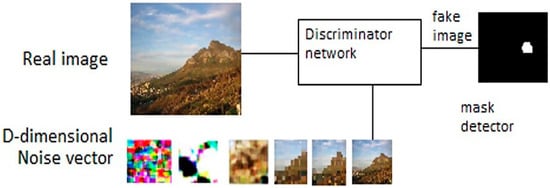
Figure 3.
The GAN module used in the proposed model.
Sample image generation: Sample outputs can be generated by untrained generators. Using Tensorflow, we first define the session and assign an input placeholder that we will refine at a later stage. Note that the loss function in GANs can be quite complex compared to standard CNN classifiers. Meanwhile, the generator constantly improves its output images, and the discriminator works to better discern “real” from “generated” images. Hence, the loss functions need to be formulated to take both networks into account. So, discriminator prediction probabilities of real dataset images will be held by ; generated images will be held by ; and discriminator prediction probabilities of the generated images will be held by .
Our goal is to generate images on the generator network that the discriminator will not be able to identify as forgeries. To achieve that end, we start by computing label-of-1 and losses using the function “tf.nn.sigmoid_cross_entropy_with_logits”. After obtaining the two loss functions (d_loss and g_loss), our next step is defining the optimizers. In the generator network, the optimizer is used to update the generator’s weights only, not the discriminator’s weights. Therefore, we need to ensure this distinction, which we can do by devising two separate lists of the generator’s weights and the discriminator’s weights. After specifying the two optimizers, the better SGD option appears to be Adam. Finally, to update our generator and get a probability score, a random z vector will be fed to the generator and the output passed to the discriminator. Discriminator updates will be obtained in the same way, substituting the discriminator for the generator.
4.3. CNN Networks
CNNs function as feature extractors. We will first use Tensorflow to create the CNNs for self-correlation, looping, and conv. layers, as in Figure 4. These will feed into the mask detector, which will highlight similarities existing throughout the target area of the image. Next, the extracted features will be subjected to self-correlation, with the module detecting any extracted features that are alike. The percentile pooling layer will then compile the relevant statistics. Finally, the mask detector will be used to recast the feature to its original image size, after which the linear classifier will be applied and a decision made regarding the authenticity of the image.
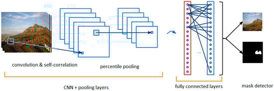
Figure 4.
The branch used for similarity detection based on CNN.
4.4. Merging Network
The outputs of these two networks serve as inputs for the merging network unit. The three core aims for building this new network are: first, to render a final decision on the copy-move forgery image under study; second, to make the copy-move transaction localized; and third, to make a distinction between the original source and the targeted regions of a potentially forged image. Though varied in their application, neural networks (NNs) are generally used to predict categorical variables. A typical neural network NN classifier features input nodes, with indicating how many values can be assumed by the dependent variable. In the present network, we use as input values the two vectors from the other network’s output. Thus, CMFD classifier output, in this case, is a node that represents the concatenated sum of all relevant inputs.
To begin, we tested all of the model networks individually. At the point where the desired outcome was obtained by the two networks, we used GAN to detect any forged area(s) in the image and the similarity CNN to detect any similar area(s). Next, the two outputs were combined into a single layer to represent novel vector inputs, with the first layer being an SVM classifier. Figure 5 shows the sequence of the steps from end-to-end according to the main framework in Figure 2. To preclude high extremes of randomness, every test was performed multiple times and involved random selection of both the test sets and the training sets, after which we averaged the results.
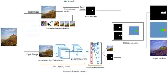
Figure 5.
Overview of the proposed two-branched, DNN-based model (GAN and CNN) ended by merging the networks to provide a CMFD solution.
The terms of expected scores are defined as
where demonstrates the case “image pristine[fake]”, is the case “decision pristine [fake]”, and indicates the predicted scores from each case [61].
- CMFD classifier: we used an SVM linear classifier. Eventually, our SVM classifier uses the merging of the vector features of the two models and is trained over the whole training set.
- Output Masking: shows three images with copy-move forgeries, the corresponding ground truth, and the detection map output from our method. Note that the forgery is easily detected, and the map is quite accurate, although the original and copied regions are distinguished from one another
With a view to making the model more robust, alternative performance measures were attempted For example, in every SVM classifier, the separating hyperplane was shifted to an orthogonal direction and the subsequent ROC was constructed. Next, we calculated the area under (the receiver operating) curve (AUC) for every model, as a sizeable AUC usually indicates robustness, even when functioning under changeable conditions [61].
The comparison between the proposed method and other state-of-the-art methods in terms of feature vector dimensions, which is presented in Table 1, shows that our method technique uses low feature vector dimensions, which in fact, increases the model efficiency in an effective syntactic computational scheme.

Table 1.
Comparison of computational complexity.
5. Proposal Implementation
This section provides details on the present study’s localization and splicing detection methods. For further details on GAN, please refer to [61]. The GAN used in this work is called CapsuleGAN, which is trained with forged and pristine images as a means to map input image in relation to forgery mask . As shown in Figure 2, the GAN architecture comprises a generator G and a discriminator D, with generator G consisting of a 16-layer U-net format of 8 encoder and 8 decoder layers [65,66]. So, for instance, if receives image , will calculate a forgery mask (soft mask) as . In doing so, the generator aims to construct an as similar as possible to the genuine . The discriminator will then differentiate between the generator’s constructs (i.e., synthesized input-mask pairs vs. genuine input-mask pairs ). Equation (4) expresses how the discriminator and generator are coupled through a loss function using cGAN. The training of the generator includes forcing it to construct masks that are so close to the original that the discriminator is unable to distinguish the original from the forged. In this way, the generator is forced to become better at creating near-identical images.
The architecture of the discriminator is a 6-layer CNN that can perform binary classification for masks. Whether an image-mask estimate pair or a genuine image-mask pair is given to the discriminator, it will subdivide the provided input as pixel patches. Every patch within the subdivision will then be classified either as pristine or forged by assigning a patch label of either 1 or 0, respectively, after which the values of every patch combined will be averaged in order to classify the complete input. We can use these equations to illustrate the two cases from the paragraph.
Essentially, what we create is a minimax game, with generator and discriminator training through the competition to enhance the skills of the other.
The coupled loss function of the network is described in the following equations:
Above, we explained how generator is forced to construct mask that can fool the discriminator , but this process stops short at guaranteeing the synthesized mask can detect an image forgery. So, for instance, if can trick the discriminator into believing it is not a forgery, it will be classified as authentic, even though it is not, and . To overcome this failure, we can then add another limitation to the generator , thus enabling it to reconstruct the genuine masks from the original training images, such that . We can accomplish this through retraining and teaching it how to minimize reconstruction losses LR related to and . Keeping in mind that our overall aim is still to categorize each pixel as either pristine or forged, is chosen as our binary cross-entropy (BCE) loss. Hence, the total loss function for cGAN can be expressed as follows:
After training has been accomplished, generator will be able to construct mask , which is very close to . Then, to evaluate forgery detection, we can estimate the mean pixel value for a mask as follows:
where is the image resolution.
Binary thresholding can then be used in tandem with threshold to decide if a specific image has been forged or not. Images are designated pristine (i.e., not forged) if , or according to thresholding, if avg. . If this is not the case, is considered a forgery.
We illustrate receiver operating characteristic (ROC) curves showing various threshold performance levels. Additionally, the ROC will indicates model performance when employing BCE loss and as reconstruction loss and illustrates that the area under the curve (AUC) designates perfect detection accuracy. The results can be verified against the precision recall (PR) plot for the model, which also shows an excellent detection rate for this work experiment.
Finding the similarity using CNN is straight-forward, as mentioned above, except when including customized layers to perform self-correlation and pooling procedures in the percentile scheme by preferencing the vector scores in percentile ranking. Each feature extracted by CNN will produce a feature tensor sized at 16 × 16 × 512. The goal here is to match any similar features by correlating all features together by applying a self-correlation layer to sort out the tensor , as follows:
where is the Pearson correlation coefficient, which, in fact, maintains the feature similarity. For instance, here we have two suspected feature patches, and , which can be normalized in the form of and . The to these designated features will be given as follows:
Here, is the mean value of the feature where is the standard deviation to the same feature and the feature size is defined by . The feature tensor now can be sorted by applying percentile pooling to new vector, called . Plotting this vector will give a curve shape. The matched features and will cause the curve to drop abruptly whenever they exist.
The vector scores in percentile ranking will fix the issue in the pooling layer input size by normalizing the score vector. This can be done by applying a percentile ranking filter through the percentile pooling layer, as shown in Figure 5. This, indeed, will reduce the scores’ dimensionality to allow using a smaller vector of the total scores. The produced mask will follow the same technique used in the above network by using the same binary classifier. The final step is determined for the source patch against the target one by using the merging network.
6. Results and Discussion
6.1. Training GAN Models in Forgery Detection
The present study proposes using a generative adversarial network (GAN) for a framework to include relevant entities. For instance, cNets has been employed as discriminators, compared to its counterparts GANs, and both of them are assessed quantitatively and qualitatively [67]. Our test results indicate a more robust performance by cGANs compared to CNN-based GANs for constructing a model that reflects how CIFAR-10 [68] and MNIST [69] datasets apply the generative adversarial metric (GAM) either quantitatively or qualitatively [70]. As discussed earlier, Goodfellow et al. [56] debuted the GANs framework in order to build a generative model for data that would learn how to transform points from simple prior distribution () to data distribution () using an adversarial generator and discriminator. The generator’s task is to learn to transform , while the discriminator is used to goad the generator into performing better . Ultimately, the discriminator must be able to distinguish between a sample from the generator’s output distribution and one derived from data distribution (), giving a scalar output .
Capsule Networks: Hinton et al. [67,71] first introduced capsules as a learning approach to robust unsupervised image representation. Capsules can be generally defined as locally invariant neuron group learning to detect visual entities in their midst and encode the properties of those entities as vector outputs. In this process, the vector length is restricted to being either 1 or 0 as an entity representation. So, for instance, the capsules are able to learn how to discern images of specific objects, or parts thereof. The neural network framework allows for the grouping of numerous capsules, creating capsule layers. In these layers, individual units generate vector outputs rather than producing traditional scalar activation. Equation (2) depicts margin loss when training CapsNets to perform multi-class classifications:
where indicates target labels , , and λ = 0.5, which represent down-weighting factors that can inhibit the shrinking of capsule output lengths in the final layer during the early-stage learning phase. Also included in the network is regularization, which appears as weighted image reconstruction loss. In this addition, the vector outputs from the final layers are manifested to the reconstruction network as inputs.
6.1.1. Data Environment
Our experimental results are provided through several datasets. As a training task, we chose the datasets CIFAR-10 and MNIST. The CIFAR-10 dataset shows 32 × 32 color images categorized as ten distinct classes (in alphabetical order: airplane, automobile, bird, cat, deer, dog, frog, horse, ship, and truck), while the MNIST dataset shows 28 × 28 hand-written grayscale images. When we test the model with additional datasets from both the forged and pristine images categories, a total of 1792 pair images will be considered, such as in the MICC-F600 dataset [72], Oxford buildings dataset, and IM dataset [70]. Also, we recommend adding more datasets for more reliability, such as ImageNet, for future extended work. Figure 6 depicts the random result samples of the proposed model.
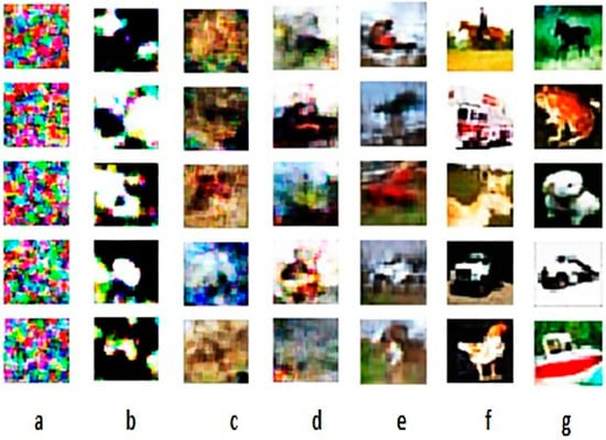
Figure 6.
From left to right, the samples from random results show the process of training improving transition results of the model using the CIFAR-10 dataset and a maximum iteration of 10,000.
As shown, the model is pretrained to ensure it has the weights to perform both generator and discriminator training tasks. The pretraining method for the discriminator is illustrated in Figure 7. As indicated, the pretraining of the generator and discriminator is not carried out simultaneously ((Pre. Disc, Pre. Gene) = (True/False) or = (False/True)). Note that although we chose to use the model’s pretraining weights to train the dataset, as well as to test the same dataset at a later time, it is possible that using alternative pretraining model weights could give the same or similar results. Figure 8, Figure 9 and Figure 10 show the training results for finding the fitting model using different datasets.
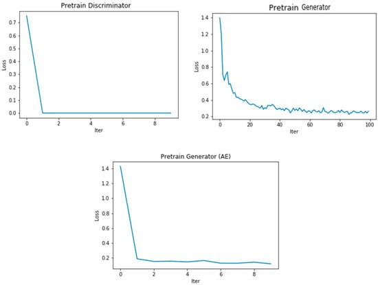
Figure 7.
The loss function of the pretraining model.
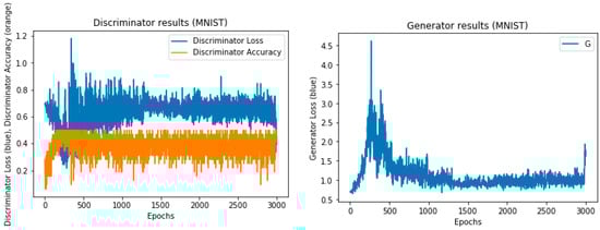
Figure 8.
The training results of the MNIST dataset with 1000 epochs.
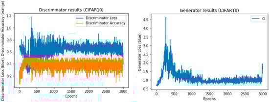
Figure 9.
The training results of the CIFAR-10 dataset with 1000 epochs.
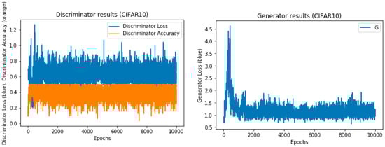
Figure 10.
The training results of the CIFAR-10 dataset with 10,000 epochs.
After training the GAN, we test the discriminator by using MNIST.
We obtain (), representing the random input image, the dimensional noise vector input, and the generator output, respectively, as shown in Figure 11 and Figure 12.
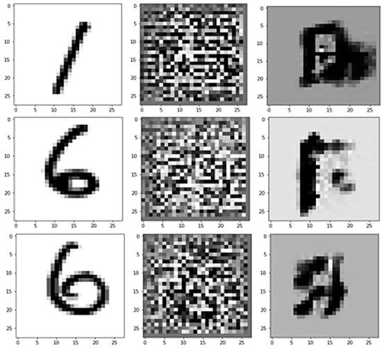
Figure 11.
The output after the first initial training stage is low quality.
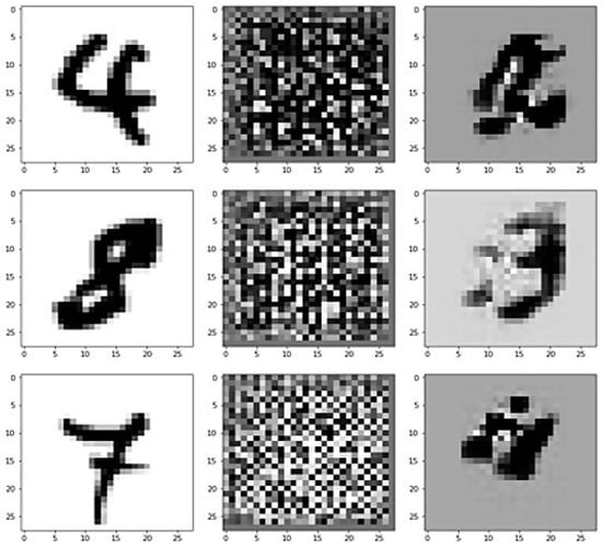
Figure 12.
Output in an advanced stage of training loops shows a closer output compared to the real input image.
6.1.2. Experimental Setup
In this work, we used a Keras GAN. Keras implementations of generative adversarial networks (GANs) are suggested in many research papers and can be found at: https://github.com/eriklindernoren/Keras-GAN. We used the TensorFlow backend for the training task.
Analysis
As was mentioned, the training tips for the combined model for the discriminator and the generator are as follows (False = 0, True = 1):
- (a)
- Train the discriminator:
- (b)
- Train the generator (to have the discriminator label samples as valid):G Loss = combined train (noise, valid)Noise = random batch on imageValid = adversarial ground truth
In this experiment, we will use two different types of training, in the following steps: (a) Use pretrained weight file (hd5) for the previous dataset. (b) Pretrain the dataset and use its own weight file (hd5). (c) Compare between the two cases. Our first task was to prepare the dataset. There are two classifications in the training dataset: forged and pristine. The paired images will be used to illustrate how the forgery operation proceeds (here, we use copy-move forgery). Prior to starting the training, pixels from multiple images are loaded into a directory using the NumPy array distribution. We begin with the pristine category and then perform tests with both forged and pristine images. To obtain a directory image file list, we import the glob, use the file list to construct two diminution matrices, and then convert the file list to a NumPy array. Thus, if we combine the total images as one NumPy array, we get:
x = np.array([np.array(Image.open(f-name)) for f-name in file-list]).
This array is divided later into three partitions for training, verification, and testing.
Figure 13 presents random samples of GAN training results in image representation. This figure shows, from left to right, the progress of generating images in different times using the CIFAR-10 dataset. From the plot in Figure 14, we can see that our model has comparable performance in training the dataset for both the pretrained discriminator and the generator. Figure 15 shows a random sample of the forgery detection result using GAN in image representation. Here, we can see the original input image, the new corresponding image, the forged image, and the output binary mask side-by-side.
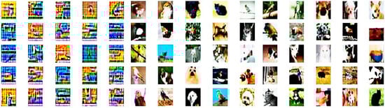
Figure 13.
From left to right, some samples from random results show the process of training improving the transition result of the model using the local dataset.
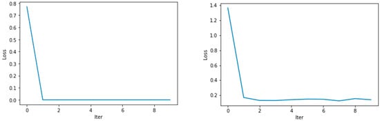
Figure 14.
Loss functions (D loss, G loss) of the training model using a custom local dataset using the pretrained discriminator and generator, respectively.
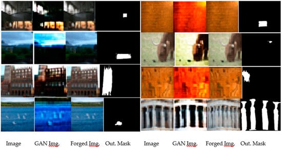
Figure 15.
Detecting the copy-move forgery using the GAN model.
6.2. Training CNN Models in Similarity Detection
In this study, a new type of deep neural network architecture was introduced for detecting and localizing copy-move forgery. The model, which uses a supervised end-to-end trainable network, was able to detect the copy-move forgery with high accuracy. Specifically, it was able to pinpoint areas in the image that were sourced from the same original area.
6.2.1. How the Model Works
The model functions as follows. First, an image is input, from which features are extracted by employing the CNN feature extractor. Next, based on the extractions, feature similarity is calculated using the self-correlation module, and statistics are gathered using percentile pooling. These then up-sample feature maps against the original image size by applying a mask decoder, after which a binary classifier creates a copy-move mask. The present research gained inspiration from a number of published works [52,59,73].
In summary, the copy-move forgery detection baseline was first developed by making feature maps from input image extracts, followed by the construction of relevant feature statistics on the basis of percentage pooling process from up-sampled feature maps. The feature classifier was then applied as a means to detect and assign similar regions as copy-move forgery areas. The subsequent tests we performed relied on a pretrained weight file for the initial model branch; later, however, we built another weight file (HD5 format), intending to compile a large number of images into a single entity. This made our training more accurate and readied the stage for the subsequent portions of the model construction.
Numerous image samples were used in the training process. A single-class classifier tested every image to determine whether it was a copy-move forgery or was pristine. Figure 16 and Figure 17 depict images that are forged, as well as a detected soft mask and a genuine mask. The test applied a set of forged images to carry out the primary task of the network branch, using recall, precision, and F1 scores to report CMFD performance. We considered the classified pixels from both the target and the source as being forged in order to compare our proposed model to other CMFD approaches that predict only binary masks.
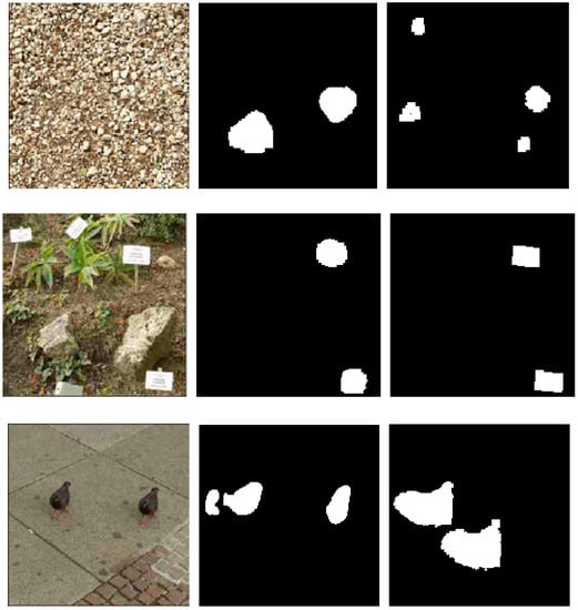
Figure 16.
Random results of similarity detection with F1 score > 0.25.
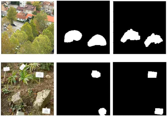
Figure 17.
Random results of similarity detection with F1 score and threshold T > 0.75.
6.2.2. Some Result Using Different Datasets
Numerical results in Table 2 show a discernibility summary of different datasets form state-of-the-art models compared to the proposed model, while Figure 18 gives a visual illustration of a similar comparison.
Table 2.
The skeleton metrics for the precision recall F scores.
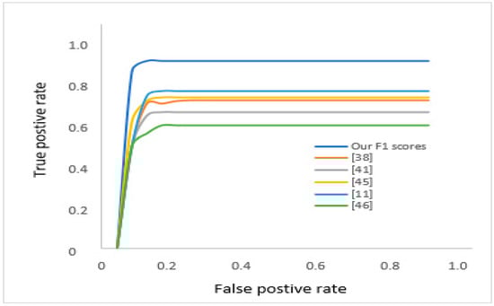
Figure 18.
The ROC for F score comparison with state-of-the-art models.
6.3. Training the CMFD Classification Model for Localization
A single support vector machine (SVM) classifier was employed in our model for all three branches for detection and classification. The outcomes indicate precision, accuracy, and good recall and F measures.
The primary aim of the model’s third branch was verifying and then localizing any detected copy-move forgery. Note that the first network uses GAN to detect and manipulate areas of the frame of the input image, whereas the second branch detects similar areas of the input image as being indicative of a copy-move forgery incidence. The third branch merges the outputs from the two other branches to produce the final results (in the step sequence shown in Figure 19), as follows:
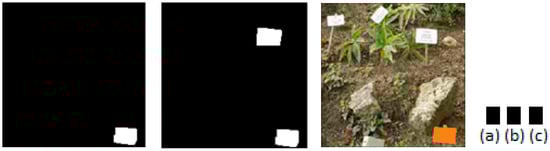
Figure 19.
(a) Masking the forged area (GAN) (. (b) Masking the similar areas in the forged image frame (CNN) (. (c) Forgery location.
(1) Verifying CMFD
Image forgery is detected by the GAN network by determining one or more interrupted areas, as detailed previously in Section 6.1. Then, as mentioned in Section 6.2, the CNN network matches similar batches in the image. This step trains the merging network to detect any forgery by comparing and testing the outputs.
(2) Localizing CMF
Following the verification of CMF detection, the model constructs a mask that pinpoints the CMFD location within the forged image frame.
Evaluating forgery localization entails a similar process in images where forgery has already been discerned. In these cases, the mask estimates indicate the threshold, but are subsequently compared (pixel-wise) with related ground truth masks . Note that the ROC curves here (Figure 20) indicate localization for various threshold levels. By applying the binary cross entropy (BCE) loss, we can see that in Table 2, the PR curve obtains 0.6963 as a mean precision score and 0.8042 as a mean recall score, confirming the strength of the localization results.
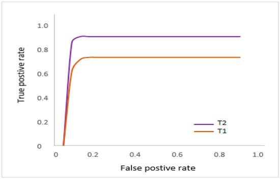
Figure 20.
Shows the ROC for F scores.
The precision recall area under the curve (AUC) (Figure 21) illustrates excellent detection accuracy. Here, the target is to have the model curve in the upper point in the right corner, which presents an ideal model with 100% true positive and zero false positive rates, regardless of recall. The area under the curve shows that perfect detection of the forgery using this model is fairly likely.
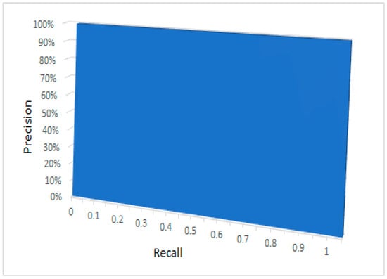
Figure 21.
Illustrates that the area under the curve (AUC).
(3) Determining the CMF Area vs. Source Area
Because the variations between the source (original) and the copy-move batch can be very small, the unaided human eye is usually unable to detect the forgery. Therefore, autodetection with a deep learning method is necessary to determine a forged image. This is especially important for discerning an original source image from a forged one. Figure 22 illustrates the source and CMF areas in various colors, making it easier for people to see the difference between the images.
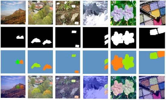
Figure 22.
The final output contributes the three main objectives of the model.
7. Conclusions
Currently, no trustworthy, commercial, real-world application exists in the market that gives an ideal solution for specific copy-move image forgery. However, there are some applications that provide a limited solution for image forgery in general, such as forensic beta [74], which works as a magnifying glass that help to see more hidden details in the image. The MagNET forensic [75] application works as an online platform to investigate metadata. The present work proposed an image analysis method that employs GAN for localization and splicing detection of images. The novel method adopts a data-driven strategy that enables the algorithm to constantly update its learning via training data to discern pristine areas from forged ones. The test results clearly indicate the significantly high accuracy of the proposed method in applying the dataset to discern localization and tampering detection. Also noteworthy is the proposed technique’s ability to project its findings to differently sized forgeries than the ones used in training. The results from these tests encourage an extension of the research to additional related inquiries, such as testing the method with other kinds of forgeries and datasets.
The rationale for the proposed CMF solution in the present work is testing the potential to train auto-encoders to acquire a representation of image patches originating from pristine images. Such an auto-encoder could also be employed in feature extraction of image patches. In the tests, a single-class SVM detects if feature vectors are derived from pristine or forged images. Generative adversarial networks are used to train the auto-encoder in detecting forgery, with the entire system being trained solely with pristine data. The system, thus, has no prior knowledge of forgeries. Even so, the test results indicate a high level of accuracy for localization as well as detections. In fact, the proposed model succeeded in its assigned CDFD task, giving performance results in the 93% to 97% range. Future related work could consider testing and enhancing system robustness by introducing a variety of different forgery types and increasing the number of used images for GAN training by including more datasets, such as ImageNet. The sensitivity of the presented methodology to the setup of its parameters should be investigated.
Author Contributions
Y.A. received his B.Sc. in 2002 in computer and telecommunication engineering from Subha University, Libya. In 2007 received his M.Sc. Electronic and Telecommunication Engineering, University Technology Malaysia UTM, Malaysia. Currently, a PhD student at Memorial University, Newfoundland, Canada. Department of Electrical and Computer Engineering. Faculty of Engineering and Applied Science. IEEE member. He conceptualized the idea, conducted the literature search and drafted the manuscript; M.T.I., B.Sc. (UET, Lahore), M.Sc. (QAU, Islamabad), Ph.D. (Imperial College London), P. Eng. Now, work supervisor and, Prof. in the Department of Electrical and Computer Engineering Faculty of Engineering and Applied Science Memorial University of Newfoundland St. John’s, Newfoundland, Canada. Senior member in IEEE. Supervised the whole process and critically reviewed the content of the manuscript; M.S., B.Sc. degree with honors in 1996, his M.Sc. degree in computer engineering in 2001 from Zagazig University, Egypt, and then his Ph.D. in 2005 from the University of Calgary, Canada. Following his Ph.D., he worked as a Post-doctoral Fellow at the University of Calgary; after that, he joined Intelliview Technologies Inc. as the Vice-President of the research and development. Shehata is currently with the department of Computer Science, Math, Physics, and Statistics at the University of British Columbia, he is also an adjunct professor in the department of Electrical and Computer Engineering at Memorial University. His research activities include computer vision, image processing, and deep learning. Supervised the process, conceptualized the general idea and reviewed the manuscript.
Funding
This research was funded by the ministry of higher education of Libyan Government, which managed by CBIE in Canada.
Acknowledgments
The authors acknowledge T. Iqbal, who made the most of the help and reviews to improve this work. Also, the authors acknowledge the Memorial University of Newfoundland laboratory facilities (MUN-LF department).
Conflicts of Interest
The authors declare that there is no actual or potential conflict of interest regarding the publication of this article. The funders had no role in the design of the study; in the collection, analyses, or interpretation of data; in the writing of the manuscript, or in the decision to publish the results.
Abbreviations
List of the abbreviations used in this study.
| Abbreviation | Explanation |
| CNN | Convolutional neural network. |
| GANs | Generative adversarial networks. |
| CMFD | Copy-move forgery detection. |
| SVM | Support vector machine. |
| PCA | Principal component analysis. |
| DCT | Discrete cosine transforms. |
| SIFT | Scale-invariant feature transform. |
| DNNs | Deep neural networks. |
| SGD | Stochastic sub-gradient descent. |
| VGG | Visual geometry group. |
| ConvNet | Convolutional network layer. |
| ReLU | Rectified linear unit layer. |
| ROC | Receiver operating characteristic. |
| AUC | The area under the curve. |
| HD5-HDF5 | Hierarchical data format. |
| F1 score | A measure of a test’s accuracy. |
| BCE | Binary cross entropy. |
| PR | Positive rate. |
| ORB | Oriented FAST and rotated BRIEF. |
| SURF | Speed up robust feature. |
| SIFT | Scale invariant feature transform. |
| VGG16 | Visual geometry group (VGG Network with 16 layers). |
| Conv | Convolutional layer. |
| cGAN | Conditional generative adversarial network. |
| cNets | Capsule network. |
| CIFAR-10 | Dataset consists of 60,000 32 × 32 color images in 10 classes. |
| MNIST | Dataset of handwritten digits with 60,000 examples. |
| MICC_F600 | Copy-move dataset composed by 660 images in total. |
References
- Rocha, A.; Scheirer, W.; Boult, T.; Goldenstein, S. Vision of the unseen: Current trends and challenges in the digital image and video forensics. ACM Comput. Surv. 2011, 43, 26. [Google Scholar] [CrossRef]
- Piva, A. An overview on image forensics. ISRN Signal Process. 2013, 2013, 22. [Google Scholar] [CrossRef]
- Stamm, C.; Wu, M.; Liu, K.J.R. Information forensics: An overview of the first decade. IEEE Access 2013, 1, 167–200. [Google Scholar] [CrossRef]
- Fridrich, A.J.; Soukal, B.D.; Lukáš, A.J. Detection of copy-move forgery in digital images. In Proceedings of the Digital Forensic Research Workshop, Cleveland, OH, USA, 6–8 August 2003. [Google Scholar]
- Ke, Y.; Sukthankar, R.; Huston, L. An efficient parts-based near-duplicate and sub-image retrieval system. In Proceeding of the 12th Annual ACM International Conference on Multimedia, New York, NY, USA, 10–16 October 2004; pp. 869–876. [Google Scholar]
- Wu, Y.; Abd-Almageed, W.; Natarajan, P. BusterNet: Detection Copy-Move Image Forgery with Source/Target Localization. In Proceedings of the European Conference on Computer Vision (ECCV), Munich, Germany, 8–14 September 2018. [Google Scholar]
- Fan, S.; Ng, T.-T.; Koenig, B.L.; Herberg, J.S.; Jiang, M.; Shen, Z.; Zhao, Q. Image Visual Realism: From Human Perception to Machine Computation. IEEE Trans. Pattern Anal. Mach. Intell. 2017, 40, 2180–2193. [Google Scholar] [CrossRef] [PubMed]
- Lyu, S.; Farid, H. How realistic is photorealistic? IEEE Trans. Signal Process. 2005, 53, 845–850. [Google Scholar] [CrossRef]
- Wu, R.; Li, X.; Yang, B. Identifying computer generated graphics VIA histogram features. In Proceedings of the 2011 18th IEEE International Conference on Image Processing, Brussels, Belgium, 11–14 September 2011; pp. 1933–1936. [Google Scholar]
- Dehnie, S.; Sencar, T.; Memon, N. Digital Image Forensics for Identifying Computer Generated and Digital Camera Images. In Proceedings of the 2006 International Conference on Image Processing, Atlanta, GA, USA, 8–11 October 2006; pp. 2313–2316. [Google Scholar]
- Dirik, A.; Bayram, S.; Sencar, H.; Memon, N. New features to identify computer generated images. In Proceedings of the 2007 IEEE International Conference on Image Processing, San Antonio, TX, USA, 16 September–19 October 2007; pp. IV-433–IV-436. [Google Scholar]
- Gallagher, A.; Chen, T. Image authentication by detecting traces of demosaicing. In Proceedings of the 2008 IEEE Computer Society Conference on Computer Vision and Pattern Recognition Workshops, Anchorage, AK, USA, 23–28 June 2008; pp. 1–8. [Google Scholar]
- Lalonde, J.-F.; Efros, A. Using color compatibility for assessing image realism. In Proceedings of the 2007 IEEE 11th International Conference on Computer Vision, Rio de Janeiro, Brazil, 14–21 October 2007; pp. 1–8. [Google Scholar]
- Zhang, R.; Wang, R.-D.; Ng, T.-T. Distinguishing photographic images and photorealistic computer graphics using visual vocabulary on local image edges. In International Workshop on Digital Forensics and Watermarking; Springer: Berlin/Heidelberg, Germany, 2011; pp. 292–305. [Google Scholar]
- Rahmouni, N.; Nozick, V.; Yamagishi, J.; Echizen, I. Distinguishing computer graphics from natural images using convolution neural networks. In Proceedings of the 2017 IEEE Workshop on Information Forensics and Security (WIFS), Rennes, France, 4–7 December 2017; pp. 1–6. [Google Scholar]
- De Rezende, E.R.; Ruppert, G.C.; Carvalho, T. Detecting Computer Generated Images with Deep Convolutional Neural Networks. In Proceedings of the 2017 30th SIBGRAPI Conference on Graphics, Patterns and Images (SIBGRAPI), Niteroi, Brazil, 17–20 October 2017; pp. 71–78. [Google Scholar]
- Holmes, O.; Banks, M.S.; Farid, H. Assessing and Improving the Identification of Computer-Generated Portraits. ACM Trans. Appl. Percept. 2016, 13, 1–12. [Google Scholar] [CrossRef]
- Shrivastava, A.; Pfister, T.; Tuzel, O.; Susskind, J.; Webb, R.; Wang, W. Learning from Simulated and Unsupervised Images through Adversarial Training. In Proceedings of the 2017 IEEE Conference on Computer Vision and Pattern Recognition (CVPR), Honolulu, HI, USA, 21–26 July 2017. [Google Scholar]
- Liu, M.-Y.; Breuel, T.; Kautz, J. Unsupervised Image-to-Image Translation Networks. In Proceedings of the Advances in Neural Information Processing Systems, Long Beach, CA, USA, 4–9 December 2017. [Google Scholar]
- Haouchine, N.; Roy, F.; Courtecuisse, H.; Nießner, M.; Cotin, S. Calipso: Physics-based image and video editing through cad model proxies. arXiv 2017, arXiv:1708.03748. [Google Scholar] [CrossRef]
- Thies, J.; Zollhofer, M.; Stamminger, M.; Theobalt, C.; Nießner, M. Face2Face: Real-Time Face Capture and Reenactment of RGB Videos. In Proceedings of the IEEE Conference on Computer Vision and Pattern Recognition, Las Vegas, NV, USA, 26 June–1 July 2016; pp. 2387–2395. [Google Scholar]
- Isola, P.; Zhu, J.-Y.; Zhou, T.; Efros, A.A. Image-to-Image Translation with Conditional Adversarial Networks. In Proceedings of the 2017 IEEE Conference on Computer Vision and Pattern Recognition (CVPR), Honolulu, HI, USA, 21–26 July 2017. [Google Scholar]
- Zhu, J.-Y.; Park, T.; Isola, P.; Efros, A.A. Unpaired Image-to-Image Translation Using Cycle-Consistent Adversarial Networks. In Proceedings of the 2017 IEEE International Conference on Computer Vision (ICCV), Venice, Italy, 22–29 October 2017. [Google Scholar]
- Farid, H. Seeing is not believing. IEEE Spectr. 2009, 46, 44–51. [Google Scholar] [CrossRef]
- Bayram, S.; Sencar, H.T.; Memon, N. An efficient and robust method for detecting copy-move forgery. In Proceedings of the 2009 IEEE International Conference on Acoustics, Speech and Signal Processing, Taipei, Taiwan, 19–24 April 2009; pp. 1053–1056. [Google Scholar]
- Cozzolino, D.; Poggi, G.; Verdoliva, L. Efficient Dense-Field Copy–Move Forgery Detection. IEEE Trans. Inf. Forensics Secur. 2015, 10, 2284–2297. [Google Scholar] [CrossRef]
- Huang, D.Y.; Huang, C.N.; Hu, W.C.; Chou, C.H. Robustness of copy-move forgery detection under high jpeg compression artifacts. Multimed. Tools Appl. 2017, 76, 1509–1530. [Google Scholar] [CrossRef]
- Mahdian, B.; Saic, S. Detection of copy–move forgery using a method based on blur moment invariants. Forensic Sci. Int. 2007, 171, 180–189. [Google Scholar] [CrossRef] [PubMed]
- Pun, C.M.; Yuan, X.C.; Bi, X.L. Image forgery detection using adaptive over-segmentation and feature point matching. IEEE Trans. Inf. Forensics Secur. 2015, 10, 1705–1716. [Google Scholar]
- Ryu, S.J.; Lee, M.J.; Lee, H.K. Detection of copy-rotate-move forgery using Zernike moments. In International Workshop on Information Hiding; Springer: Berlin/Heidelberg, Germany, 2010; Volume 6387, pp. 51–65. [Google Scholar]
- Ardizzone, E.; Bruno, A.; Mazzola, G. Copy–Move Forgery Detection by Matching Triangles of Keypoints. IEEE Trans. Inf. Forensics Secur. 2015, 10, 2084–2094. [Google Scholar] [CrossRef]
- Manu, V.; Mehtre, B.M. Detection of copy-move forgery in images using segmentation and surf. In Advances in Signal Processing and Intelligent Recognition Systems; Springer: Cham, Switzerland, 2016; pp. 645–654. [Google Scholar]
- Shivakumar, B.; Baboo, S. Detection of region duplication forgery in digital images using surf. Int. J. Comput. Sci. Issues 2011, 8, 199–205. [Google Scholar]
- Silva, E.A.; Carvalho, T.; Ferreira, A.; Rocha, A. Going deeper into copy-move forgery detection: Exploring image telltales via multi-scale analysis and voting processes. J. Vis. Commun. Image Represent. 2015, 29, 16–32. [Google Scholar] [CrossRef]
- Costanzo, A.; Amerini, I.; Caldelli, R.; Barni, M. Forensic Analysis of SIFT Keypoint Removal and Injection. IEEE Trans. Inf. Forensics Secur. 2014, 9, 1450–1464. [Google Scholar] [CrossRef]
- Yang, B.; Sun, X.; Guo, H.; Xia, Z.; Chen, X. A copy-move forgery detection method based on CMFD-SIFT. Multimed. Tools Appl. 2017, 77, 837–855. [Google Scholar] [CrossRef]
- Amerini, I.; Ballan, L.; Caldelli, R.; Del Bimbo, A.; Serra, G. A SIFT-Based Forensic Method for Copy–Move Attack Detection and Transformation Recovery. IEEE Trans. Inf. Forensics Secur. 2011, 6, 1099–1110. [Google Scholar] [CrossRef]
- Li, J.; Li, X.; Yang, B.; Sun, X. Segmentation-based image copy-move forgery detection scheme. IEEE Trans. Inf. Forensics Secur. 2015, 10, 507–518. [Google Scholar]
- Birajdar, G.K.; Mankar, V.H. Digital image forgery detection using passive techniques: A survey. Digit. Investig. 2013, 10, 226–245. [Google Scholar] [CrossRef]
- Asghar, K.; Habib, Z.; Hussain, M. Copy-move and splicing image forgery detection and localization techniques: A review. Aust. J. Forensic Sci. 2017, 49, 281–307. [Google Scholar] [CrossRef]
- Soni, B.; Das, P.; Thounaojam, D. Cmfd: A detailed review of block-based and key feature-based techniques in image copy-move forgery detection. IET Image Process. 2017, 12, 167–178. [Google Scholar] [CrossRef]
- Warif, N.B.A.; Wahab, A.W.A.; Idris, M.Y.I.; Ramli, R.; Salleh, R.; Shamshirband, S.; Choo, K.-K.R. Copy-move forgery detection: Survey, challenges and future directions. J. Netw. Comput. Appl. 2016, 75, 259–278. [Google Scholar] [CrossRef]
- Zheng, Y.; Zhou, Y.; Zhou, H.; Gong, X. Ultrasound image edge detection based on a novel multiplicative gradient and canny operator. Ultrason. Imaging 2015, 37, 238–250. [Google Scholar] [CrossRef] [PubMed]
- Cai, J.; Huang, P.; Chen, L.; Zhang, B. An efficient circle detection not relying on edge detection. Adv. Space Res. 2016, 57, 2359–2375. [Google Scholar] [CrossRef]
- Zhang, Z.; Liu, Y.; Liu, T.; Li, Y.; Ye, W. Edge Detection Algorithm of a Symmetric Difference Kernel SAR Image Based on the GAN Network Model. Symmetry 2019, 11, 557. [Google Scholar] [CrossRef]
- Luan, S.; Chen, C.; Zhang, B.; Han, J.; Liu, J. Gabor Convolutional Networks. IEEE Trans. Image Process. 2018, 27, 4357–4366. [Google Scholar] [CrossRef] [PubMed]
- Park, K.; Kim, D.H. Accelerating Image Classification using Feature Map Similarity in Convolutional Neural Networks. Appl. Sci. 2019, 9, 108. [Google Scholar] [CrossRef]
- Hsu, C.C.; Lee, C.Y.; Zhuang, Y.X. Learning to Detect Fake Face Images in the Wild. In 2018 International Symposium on Computer, Consumer and Control (IS3C); IEEE: Piscataway, NJ, USA, 2018; pp. 1–4. [Google Scholar]
- Snape, P.; Pszczolkowski, S.; Zafeiriou, S.; Tzimiropoulos, G.; Ledig, C.; Rueckert, D. A Robust Similarity Measure for Volumetric Image Registration with Outliers. Image Vis. Comput. 2016, 52, 97–113. [Google Scholar] [CrossRef]
- Liu, Y.; Guan, Q.; Zhao, X. Copy-move forgery detection based on convolutional kernel network. Multimed. Tools Appl. 2017, 77, 18269–18293. [Google Scholar] [CrossRef]
- Bunk, J.; Bappy, J.H.; Mohammed, T.M.; Nataraj, L.; Flenner, A.; Manjunath, B.; Chandrasekaran, S.; Roy-Chowdhury, A.K.; Peterson, L. Detection and localization of image forgeries using resampling features and deep learning. In Proceedings of the 2017 IEEE Conference on Computer Vision and Pattern Recognition Workshops (CVPRW), Honolulu, HI, USA, 21–26 July 2017; pp. 1881–1889. [Google Scholar]
- Wu, Y.; Abd-Almageed, W.; Natarajan, P. Deep matching and validation network: An end-to-end solution to constrained image splicing localization and detection. In Proceedings of the 2017 ACM on Multimedia Conference, Mountain View, CA, USA, 23–27 October 2017; Volume MM’17, pp. 1480–1502. [Google Scholar]
- Zhou, P.; Han, X.; Morariu, V.I.; Davis, L.S. Two-Stream Neural Networks for Tampered Face Detection. In Proceedings of the 2017 IEEE Conference on Computer Vision and Pattern Recognition Workshops (CVPRW), Honolulu, HI, USA, 21–26 July 2017; pp. 1831–1839. [Google Scholar]
- Dang, L.; Hassan, S.; Im, S.; Lee, J.; Lee, S.; Moon, H. Deep learning based computer generated face identification using a convolutional neural network. Appl. Sci. 2018, 8, 2610. [Google Scholar] [CrossRef]
- Zhu, Y.; Shen, X.; Chen, H. Copy-move forgery detection based on a scaled orb. Multimed. Tools Appl. 2016, 75, 3221–3233. [Google Scholar] [CrossRef]
- Goodfellow, I.; Pouget-Abadie, J.; Mirza, M.; Xu, B.; Warde-Farley, D.; Ozair, S.; Courville, A.; Bengio, Y. Generative adversarial nets. In Proceedings of the Advances in Neural Information Processing Systems, Montreal, QC, Canada, 8–13 December 2014; pp. 2672–2680. [Google Scholar]
- Nataraj, L.; Mohammed, T.M.; Manjunath, B.S.; Chandrasekaran, S.; Flenner, A.; Bappy, J.H.; Roy-Chowdhury, A.K. Detecting GAN generated fake images using co-occurrence matrices. arXiv 2019, arXiv:1903.06836. [Google Scholar]
- Marra, F.; Gragnaniello, D.; Cozzolino, D.; Verdoliva, L. Detection of GAN-generated Fake Images over Social Networks. In Proceedings of the IEEE Conference on Multimedia Information Processing and Retrieval, Miami, FL, USA, 10–12 April 2018; pp. 384–389. [Google Scholar]
- Carey, O. Generative Adversarial Networks GANs. 2018. Available online: http://towardsdatascience.com/generative-adversarial-networks-gans-a-beginners-guide-5b38eceece24 (accessed on 19 February 2019).
- Bupe, C. Why Is SVM Not Popular Nowadays; University of Zambia: Lusaka, Zambia, 2018; Available online: https://www.quora.com/ (accessed on 25 April 2019).
- Cozzoline, D.; Gragnaniello, D.; Verdoliva, L. Image forgery detection based on the fusion of machine learning and block-matching methods. Computer Science—Computer Vision and Pattern Recognition. arXiv 2013, arXiv:1311.6934C. [Google Scholar]
- Popescu, A.C.; Farid, H. Exposing Digital Forgeries by Detecting Duplicated Image Regions; Tech. Rep. TR2004-515; Dartmouth College: Hanover, NH, USA, 2004. [Google Scholar]
- Huang, Y.; Lu, W.; Sun, W.; Long, D. Improved DCT-based detection of copy-move forgery in images. Forensic Sci. Int. 2011, 206, 178–184. [Google Scholar] [CrossRef] [PubMed]
- Mahmood, T.; Nawaz, T.; Irtaza, A.; Ashraf, R.; Shah, M. Copy-Move Forgery Detection Technique for Forensic Analysis in Digital Images. Math. Probl. Eng. 2016, 2016, 1–13. [Google Scholar] [CrossRef]
- Yarlagadda, S.K.; Güera, D.; Bestagini, P.; Maggie Zhu, F.; Tubaro, S.; Delp, E.J. Satellite Image Forgery Detection and Localization Using GAN and One-Class Classification. arXiv 2018, arXiv:1802.04881v1. [Google Scholar]
- Ronneberger, O.; Fischer, P.; Brox, T.N. Convolutional networks for biomedical image segmentation. In Proceedings of the International Conference on Medical Image Computing and Computer-Assisted Intervention, Munich, Germany, 5–9 October 2015; pp. 234–241. [Google Scholar]
- Sabour, S.; Frosst, N.; Hinton, G.E. Dynamic routing between capsules. In Proceedings of the Advances in Neural Information Processing Systems, Long Beach, CA, USA, 4–9 December 2017; pp. 3859–3869. [Google Scholar]
- Krizhevsky, A. Learning Multiple Layers of Features from Tiny Images; University of Toronto: Toronto, ON, Canada, 2009. [Google Scholar]
- LeCun, Y.; Bottou, L.; Bengio, Y.; Haffner, P. Gradient-based learning applied to document recognition. Proc. IEEE 1998, 86, 2278–2324. [Google Scholar] [CrossRef]
- Jing, W.; Hongbin, Z. Exposing digital forgeries by detecting traces of image splicing. In 2006 8th International Conference on Signal Processing; IEEE: Piscataway, NJ, USA, 2006; Volume 2. [Google Scholar]
- Hinton, G.E.; Krizhevsky, A.; Wang, S.D. Transforming auto-encoders. In International Conference on Artificial Neural Networks; Springer: Berlin/Heidelberg, Germany, 2011; pp. 44–51. [Google Scholar]
- Mahendran, A.; Vedaldi, A. Visualizing deep convolutional neural networks using natural pre-images. Int. J. Comput. Vis. 2016, 12, 233–255. [Google Scholar] [CrossRef]
- Dwibedi, D.; Misra, I.; Hebert, M. Cut, paste and learn: Surprisingly easy synthesis for instance detection. In Proceedings of the IEEE International Conference on Computer Vision (ICCV), Venice, Italy, 22–29 October 2017. [Google Scholar]
- Wagner, Forensically Beta, 16 08 2015. Available online: https://29a.ch/photo-forensics/#forensic-magnifier (accessed on 28 August 2019).
- McQuaid, J. MagNet. 2015. Available online: https://www.magnetforensics.com/for-forensic-examiners/ (accessed on 28 August 2019).
© 2019 by the authors. Licensee MDPI, Basel, Switzerland. This article is an open access article distributed under the terms and conditions of the Creative Commons Attribution (CC BY) license (http://creativecommons.org/licenses/by/4.0/).