Visual Saliency Prediction Based on Deep Learning


1
Faculty of Engineering & Applied Science, Memorial University, St. John’s, Newfoundland, NL A1B 3X5, Canada
2
Faculty of Engineering, Elmergib University, Khoms 40414, Libya
3
Department of Computer Science, Mathematics, Physics and Statistics, University of British Columbia, Okanagan Campus, Kelowna, BC V1V 1V7, Canada
4
C-CORE, Captain Robert A. Bartlett Building, Morrissey Road, St. John’s, Newfoundland, NL A1C 3X5, Canada
*
Author to whom correspondence should be addressed.
Information 2019, 10(8), 257; https://doi.org/10.3390/info10080257
Submission received: 25 May 2019
/
Revised: 30 July 2019
/
Accepted: 8 August 2019
/
Published: 12 August 2019
Abstract
:Human eye movement is one of the most important functions for understanding our surroundings. When a human eye processes a scene, it quickly focuses on dominant parts of the scene, commonly known as a visual saliency detection or visual attention prediction. Recently, neural networks have been used to predict visual saliency. This paper proposes a deep learning encoder-decoder architecture, based on a transfer learning technique, to predict visual saliency. In the proposed model, visual features are extracted through convolutional layers from raw images to predict visual saliency. In addition, the proposed model uses the VGG-16 network for semantic segmentation, which uses a pixel classification layer to predict the categorical label for every pixel in an input image. The proposed model is applied to several datasets, including TORONTO, MIT300, MIT1003, and DUT-OMRON, to illustrate its efficiency. The results of the proposed model are quantitatively and qualitatively compared to classic and state-of-the-art deep learning models. Using the proposed deep learning model, a global accuracy of up to 96.22% is achieved for the prediction of visual saliency.
1. Introduction
Humans have a strong ability to pay attention to a specific part of an image instead of processing the entire image. This phenomenon of visual attention has been studied for over a century [1]. Visual attention is defined as the processes that enable an observer to focus on selected aspects of the retinal image over non-selected aspects. In other words, visual attention refers to a set of cognitive procedures that select relevant information and filter out irrelevant information from cluttered visual scenes. The task of visual attention prediction is a popular research area in the computer vision and neuroscience fields. In general, Visual Attention (HVA) is based on two strategies: bottom-up and top-down visual attention. Bottom-up models mainly employ low-level cues, such as color, intensity, and texture. Additionally, the bottom-up strategy tries to select regions which show the prominent characteristics of their surroundings [2,3]. In contrast, top-down approaches are task-oriented and try to locate a target object from a specific category. They also depend on the features of the object of interest [4,5]. Accordingly, bottom-up and top-down approaches are mainly driven by the visual characteristics of a scene and the task of interest, respectively [6,7].
In the last few years, several models have been proposed for the prediction of human visual saliency, with the most common technique being a saliency map. Saliency maps illustrate that the location of human attention is focused on a particular area within the whole image [8,9,10]. In addition, a saliency map is an image that shows each pixel’s unique quality. Importantly, the purpose of a saliency map is to change the representation of an image to a smooth image that is more meaningful and easier to analyze [11,12].
Deep Convolutional Neural Networks (CNNs) have been commonly used in the field of visual attention. This is because CNNs are strong visual models and they are able to learn features from a raw image dataset (low-level feature) and create a feature map (high-level feature) [13,14]. This scenario describes how the human visual system can detect the location of visual attention. In the last few years, several deep learning models have been used to predict visual saliency points, most of which have achieved impressive performances compared to conventional methods [15,16,17,18]. The task of extracting a saliency map has further opened the door for several applications, especially in computer vision, including object detection, object recognition, scene classification, video understanding, and image compression [19].
This study aims to propose the application of a semantic segmentation model based on the VGG-16 network (see Section 2.1 for more details on the VGG-16 network) to predict human visual attention in the field of view. Specifically, the main objective of this research is to improve the accuracy of visual saliency prediction by proposing a fully convolutional neural network-based model.
The proposed method that we used falls under the bottom-up category. Therefore, in the results section, we only compare our proposed method with relevant bottom-up methods (see Section 4.1 for more details on relevant methods).
The proposed model was developed based on the encoder-decoder architecture, wherein the fine-tuning strategy was applied in the encoder stage (i.e., VGG-16 model) [20]. More specifically, this study uses a VGG-16 model that was trained on more than a million images from the ImageNet database [20,21]. In addition, we trained the proposed model using SALICON images (see Section 3.3.1 for more details on the SALICON dataset) and their ground truth data [22], and evaluated the results over several datasets, including TORONTO, MIT300, MIT1003, and DUT-OMRON [23,24,25]. The contributions of this paper can be summarized in the following points:
- (1)
- A deep learning architecture based on the VGG-16 network that is able to predict visual saliency is proposed. As opposed to the current state-of-the-art technique that uses three stages in the encoder/decoder architecture [26], the proposed network uses five encoder and decoder stages to produce a useful saliency map (e.g., visual saliency). This makes the proposed architecture more powerful for extracting more specific deep features;
- (2)
- The proposed model is the first to use a semantic segmentation technique within the encoder-decoder architecture to classify all image pixels into the appropriate class (foreground or background), where the foreground is most likely a salient object;
- (3)
- The proposed model is evaluated using four well-known datasets, including TORONTO, MIT300, MIT1003, and DUT-OMRON. The proposed model achieves a reasonable result, with a global accuracy of 96.22%.
To this end, the proposed method, based on the VGG-16 network, is described in Section 2; the materials and methods of the proposed model in Section 3; and the quantitative and qualitative experimental results obtained from the four datasets are explained in Section 4. Finally, we summarize our results in the conclusion and report potential future uses, applications, and improvements to this research in Section 5 (Our source code is available at: https://github.com/Bashir2020/Saliency-_model_-2019).
2. The Proposed Method
The proposed model is based on a semantic segmentation technique using the VGG-16 network. Hereby, we thoroughly explain all the important information about the VGG-16 network in the next sub-sections.
2.1. The VGG-16 Netwok Architecture
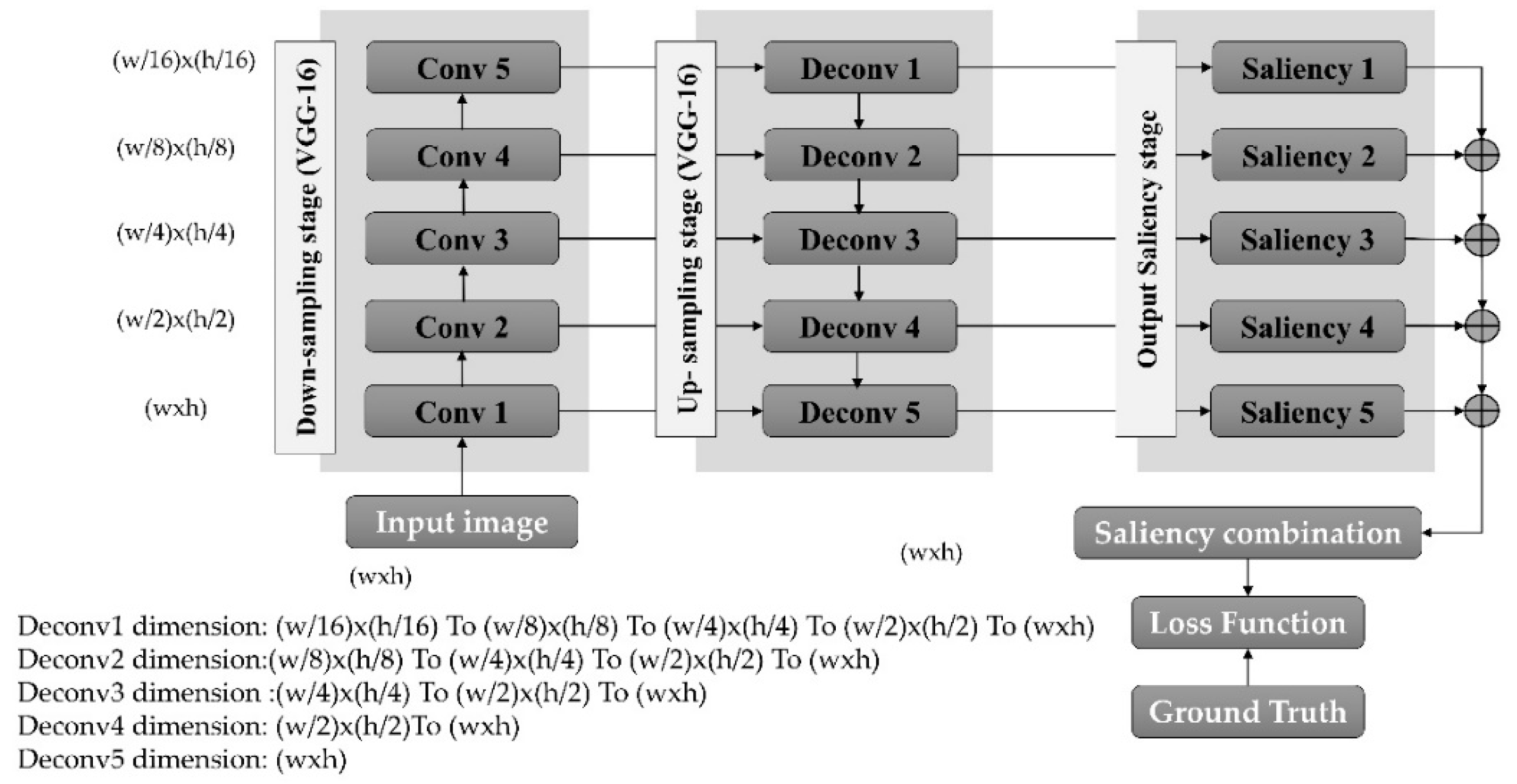
In this section, we describe the architecture of the proposed model. Our model architecture consists of encoder-decoder stages; the encoder stage has five convolutional blocks (conv1, conv2, conv3, conv4, and conv5). The encoder blocks are learned by down-sampling, which applies different receptive field sizes to create the feature maps. The decoder stage also has five deconvolution blocks (decon1, decon2, decon3, decon4, and decon5). The decoder blocks up-sample the feature maps and this creates an output the same size as the input image. The encoder blocks are adopted from a pretrained network called VGG-16 [21].
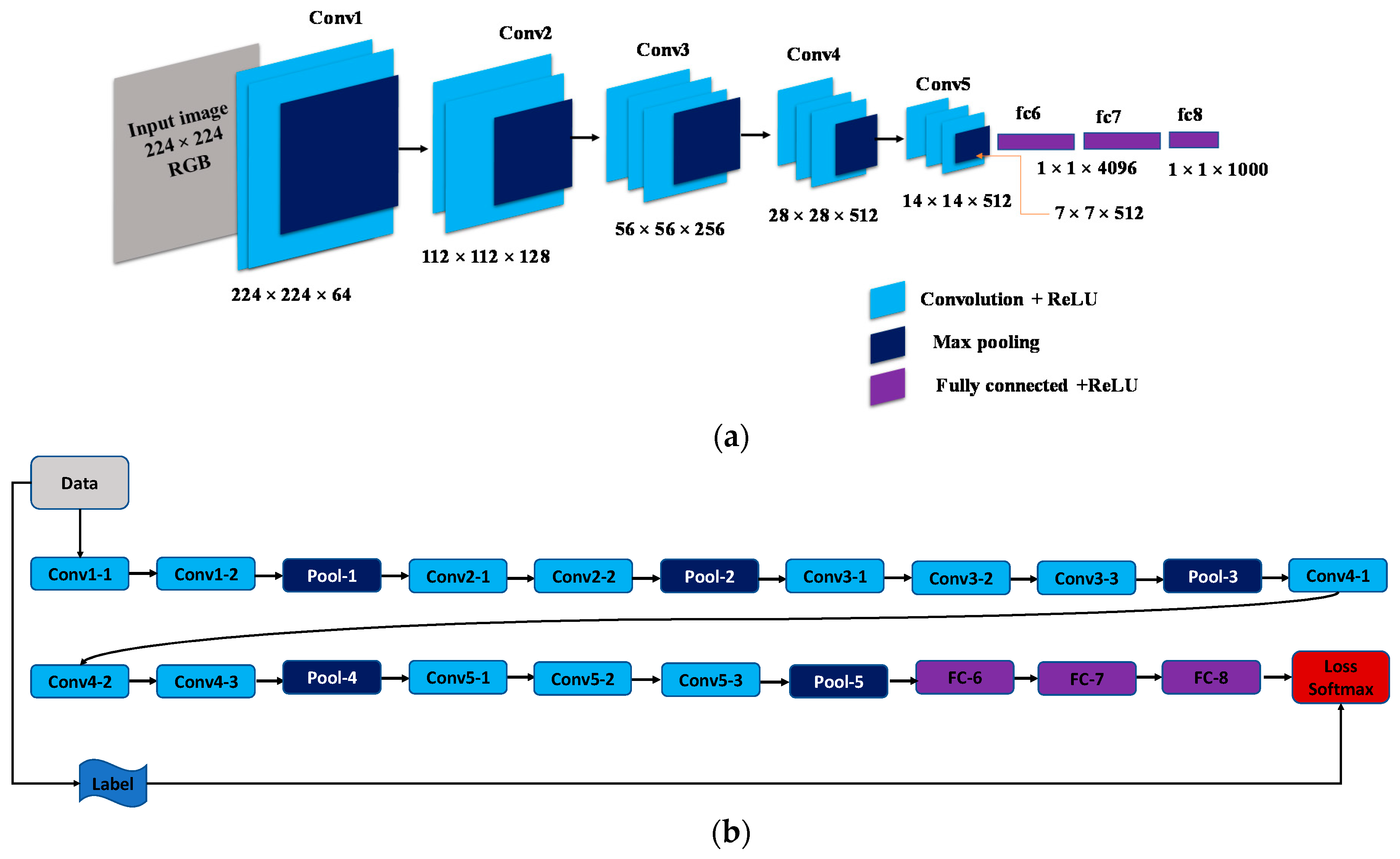
The VGG-16 network was developed by Simonyan and Zisserman in the 2014 ILSVRC competition [20]. Generally, the VGG-16 network contains thirteen convolution layers, five pooling layers, and three fully connected layers [27]. The VGG-16 network is trained on more than a million images from the ImageNet database [28] and can classify images into 1000 object classes. The VGG-16 network has an image input size of 224 × 224. Figure 1a,b shows the general structure and the data flow through the VGG-16 network.
The major difference between the VGG-16 network and previous networks is the use of a series of convolution layers with small receptive fields (3 × 3) in the first layers instead of a few layers. This results in fewer parameters and more nonlinearities in between, making the decision function more selective and the model easier to apply for training [20].
The input image is passed over a series of convolution layers with 3 × 3 convolutional filters. This is beneficial because the filter will capture the notation of the center, left/right, and up/down. The convolution stride is set to 1 pixel, whereas the padding is set to 1 pixel. Five max-pooling layers are used after convolution layers for the down-sampling operation (i.e., dimensionality reduction). Each max-pooling is also performed over 2 × 2 pixels, with a stride value of 2. In addition, three fully-connected (FC) layers follow a series of convolution layers. Specifically, the first two have 4096 channels each, and the third has 1000 channels. The structure of the fully connected layers is the same in all networks. The final layer is a soft-max layer that must have the same number of nodes as the output layer. The function of the soft-max layer is to map the non-normalized output to probability distribution through predicted output classes [20].
The convolutional neural network can be considered as the composition of several functions, as follows:
where each function takes a datum xL and parameter vector as the input and produces a datum as the output. The parameters are learned from the input data for solving a specific problem, for example, image classification. Moreover, there is a function called non-linear activation (i.e., not linear function) that is associated with the convolution layers. This function is also used to keep all the input values of the network as the positive value. Equation (2) explains this concept.
There is another important operator also associated with the architecture of the VGG-16 network that is called the pooling operator. The purpose of this operator is to reduce the dimension of the input volume (i.e., sub-sampling method) and preserve discriminant information. There are several types of operator, such as max-pooling, average-pooling, and sum-pooling. For instance, the output of a max-pooling operator is
2.2. Visual Saliency Prediction Model
In this section, we propose a visual saliency prediction model based on a semantic segmentation algorithm, where the fixation map is modeled as the foreground (salient object). A semantic segmentation algorithm classifies and labels every pixel in an image into objects (foreground) and the background [29]. There are many applications for semantic segmentation, including road segmentation for autonomous driving and cancer cell segmentation for medical diagnosis.
The architecture of the proposed semantic segmentation model is illustrated in Figure 2. To obtain a multi-level prediction, each output of the convolution layer (encoder) must be directly connected to the corresponding deconvolution layer (decoder). In general, the task of visual attention uses a combination of low-level and high-level features. In other words, we incorporate multi-layer information together to produce the output saliency map. Low-level features, such as edges, corners, and orientations, are captured by small-level receptive fields, while high-level features, such as semantic information (e.g., object parts or faces), are extracted by high-level receptive fields. Moreover, there are many receptive field sizes, and each corresponds to the layer size. Therefore, based on the advantages of CNNs, we can use small and high receptive fields in down-sampling (e.g., multi-convolution layers, such as in the VGG-16 network) to create feature maps. Both low- and high-level features are very important for predicting human visual saliency. Therefore, our proposed model produces the final saliency map based on a combination of all the outputs of the individual deconvolution operations. Additionally, in our proposed model, we only consider the CNN layers that create feature maps and we exclude the fully connected layers. In addition, the saliency combination block represents the merged multi-layer output saliency predictions (i.e., the prediction average achieves a higher performance compared to that of a single-layer output).
Assume we have an input image, and its feature map is of the l-th layer and the convolution processes are specified by the weight, . Therefore, the output of the feature map can be calculated by
where is the input image, the symbol * indicates the convolution operation, and L is the number of layers. The deconvolution operation is opposed to the convolution operation and these can be run in two directions (forward and backward through of convolution), where it performs the up-sampling operation represented by Equation (5):
where is the stride convolution and s is an up-sampling factor. The output operation of the decoder is then given as follows:
where is the deconvolution operation and is the kernel weight of the deconvolution layer. Moreover, the total number of weights can be explained by
where M represents the output prediction maps. Additionally, the loss-function is a Stochastic Gradient Descent with Momentum (SGDM, Equation (8)). The objective of this function is to accelerate gradient vectors in the right direction and increase the speed of convergence. In other words, SGDM optimizes the differentiable function and decreases classification errors [26,30]. The loss function can also be defined by Equation (8):
where is the cross entropy between the predicted probability and the ground truth (GT) labeled .
3. Materials and Methods
In this section, we describe all the steps for implementing our work, including training, adjusting the parameters of, validating, and testing the model with several available benchmark datasets (TORONTO, MIT300, MIT1003, and DUT-OMRON).
3.1. Model Training
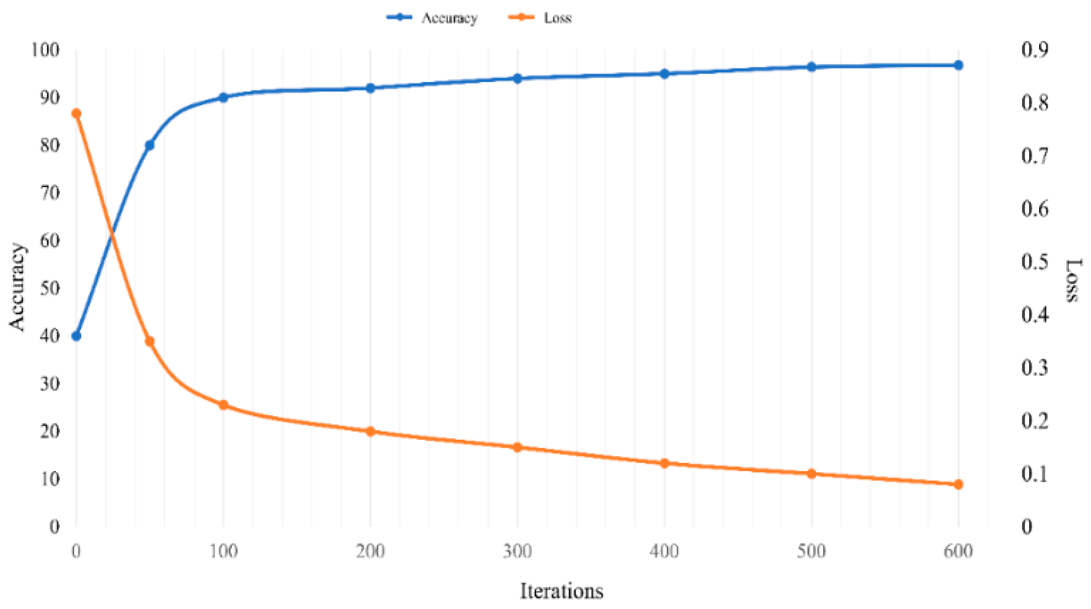
The proposed model was trained on a standard dataset (i.e., SALICON) [22]. This dataset consists of a training dataset (10,000 images) and validation dataset (5000 images), both with ground truth data and a test dataset (5000 images) without ground truth data. All the images are in JPG format, except for the ground truth dataset, which is in grayscale PNG format, and all images have a resolution of 640 × 480. At the beginning of the training, all the weights of the filters were initialized based on the pre-trained network (VGG-16), which has an input image of 224 × 224 and a Gaussian distribution with a 0.01 standard deviation and zero mean for the weights of each layer [22]. The purpose of using the VGG-16 pre-trained network is to transfer the learned knowledge and reuse it to predict human visual saliency. Additionally, the network parameters were as follows: Initial Learn Rate: 0.01; Max Epochs: 10; Mini Batch Size: 10; and number of iterations: 620. The network was trained on 10,000 images and used selected images from the test datasets for testing (the global accuracy of the proposed model was 96.22%). Moreover, using the loss function (SGDM), the model parameters learned to increase the speed of convergence and to decrease output errors. Figure 3 illustrates the training progress produced by the proposed model from the specified training images (SALICON).
3.2. Model Testing
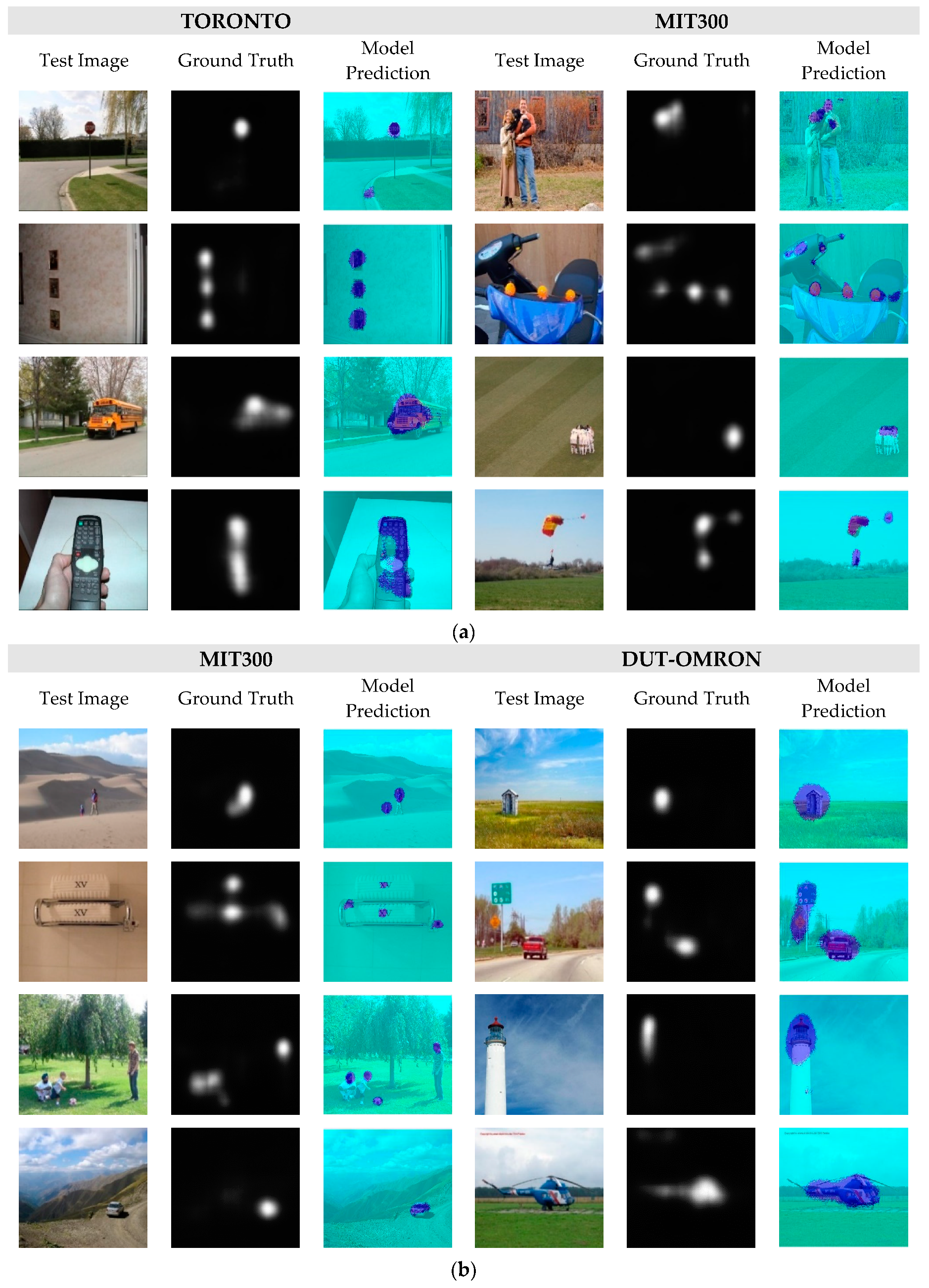
This section is devoted to testing the proposed model with several dataset images (test images). As we illustrated in the previous section, the SALICON test images are available without ground truth, thus, we suggested the use of other datasets, such as TORONTO, MIT300, MIT1003, and DUT-OMRON datasets, for model testing. Figure 4 shows the model testing of the selected images. Note that the proposed model has the ability to detect the most salient objects in the scene.
3.3. Datasets
The proposed model was tested on several well-known datasets, including TORONTO, MIT 300, MIT1003, and DUT-OMRON, which are described below. During the model testing, given an inquiry image, we obtained the saliency map prediction from the last saliency combination layer. The average time required to test an image was about 15 s.
3.3.1. SALICON
SALICON is the largest dataset for visual attention on the popular Microsoft Common Objects in context (MS COCO) image database [22]. It contains 10,000 training images, 5000 validation images, and 5000 testing images, with a fixed resolution of 480 × 640, collected from the Microsoft COCO dataset. This dataset also includes the ground truth data for the training and validation datasets; however, the ground truth data for the test datasets were not available [22].
3.3.2. TORONTO
The TORONTO dataset contains 120 colour images with a fixed resolution of 511 × 681 pixels. This dataset contains both indoor and outdoor environments and was free-viewed by 20 human subjects [24].
3.3.3. MIT300
MIT300 is a collection of 300 images that contains the eye movement data of 39 observers. It should be noted that MIT300 is a challenging dataset since its images are highly varied and natural. Saliency maps of all images are withheld and employed by the MIT Saliency Benchmark for model evaluation (http://saliency.mit.edu/results_mit300.html) [31].
3.3.4. MIT1003
MIT1003 is a collection of 1003 images from the Flicker and LabelMe collections. Saliency maps were also obtained from the eye-tracking data of 15 users. It is the largest eye fixation dataset, wherein there are 779 landscapes and 228 portraits images that vary in size from 405 × 405 to 1024 × 1024 pixels [31].
3.3.5. DUT-OMRON
DUT-OMRON contains 5168 high quality images that were manually selected from more than 140,000 images. Images in this database have one or more salient objects and a relatively complex background [32].
3.4. Evaluation Metrics
There are several indices for evaluation metrics to measure the agreement between visual saliency and model prediction. There are also previous studies on saliency metrics, which explain that it is hard to perform a fair comparison to evaluate saliency models using one metric [33]. In general, saliency evaluation indices are divided into location-based and distribution-based metrics. The former type of evaluation considers the saliency map at district locations; the latter considers both predicted saliency and human eye fixation maps as continuous distributions. The most well-known location-based indices are the Area Under the Receiver Operating Characteristic (ROC) curve in two versions of Judd and Borji [29]. Alternatively, the most commonly used distribution-based indices are the Normalized Scanpath Saliency (NSS) and Similarity Metrics (SIM). These indices are described in detail in the following sections [29].
3.4.1. Normalized Scanpath Saliency (NSS)
The NSS metric was introduced to the saliency community as a simple correspondence measure between human eye fixation and model prediction. NSS is susceptible to false positives and relative differences in saliency across the image. Given a saliency map S and a binary map of fixation location F, then
where
where N is the total number of human eye positions and is the standard deviation.
3.4.2. Similarity Metric (SIM)
The similarity metric (SIM) uses the normalized probability distributions of the saliency and human eye fixation maps. SIM is calculated as the sum of the minimum values of each pixel. The similarity between these two maps is calculated as
where and are the normalized saliency map and the fixation map, respectively. A similarity score between zero and one indicates that the distributions are the same and that they do not overlap.
3.4.3. Judd Implementation (AUC-Judd)
The AUC-Judd metric is widely used to evaluate saliency models. The saliency map is treated as a binary classifier to separate positive from negative samples at various thresholds. The true positive (tp) rate is the proportion of the saliency map’s values above a certain threshold at fixation locations. The false positive (fp) rate is the proportion of the saliency map’s values that occur above the threshold of non-fixated pixels. In this implementation, the thresholds are sampled from the saliency map’s values [34,35].
3.4.4. Borji Implementation (AUC-Borji)
The AUC-Borji metric uses a uniform random sample of image pixels as negatives and defines the fixation map’s (saliency map) values above the threshold of these pixels as false positives. This version of the Area Under ROC curve measurement is based on Ali Borji’s code. The saliency map is treated as a binary classifier to separate positive from negative samples at various thresholds. The true positive (TP) rate is the proportion of the saliency map’s values above the threshold of fixation locations. The false positive (FP) rate is the proportion of the saliency map’s values that occur above the threshold sampled from random pixels (as many samples as fixations, sampled uniformly from all image pixels). In this implementation, threshold values are sampled at a fixed step size [36].
3.4.5. Semantic Segmentation Metrices
These metrices are used to evaluate the prediction results against the ground truth data. In this study two different semantic segmentation matrices are used, which Global Accuracy and Weighted Intersection over Union (WeightedIoU). Specifically, the Global Accuracy is the ratio of correctly classified pixels, regardless of class, to the total number of pixels, and the WeightedIoU is the average IoU of all classes, weighted by the number of pixels in the class, wherein the MeanIoU is the average IoU score of all classes in that particular image [34,37].
4. Experimental Results
4.1. Quantitative Comparison of the Proposed Model with other State-of-the-Art Models
To evaluate the efficiency of the proposed model, we compared it to six state-of-the-art models. We selected four dataset benchmarks (TORONTO, MIT300, MIT1003, and DUT-OMRON) for a comparison of the quantitative results. These results are reported in Table 1, Table 2, Table 3 and Table 4, respectively.
Table 1 shows that, with the TORONTO dataset, the proposed model outperforms the other six models in terms of the NSS, AUC-Judd, and AUC-Borji metrics; however, in terms of the SIM (similarity) metric, the DVA algorithm [26] has the best results. This is because the SIM metric is better suited for non-binary classifiers. However, the proposed algorithm is a binary classifier. The other metrics used in the study (NSS, AUC-Judd, and AUC-Borji) are all binary classifier metrics.
From Table 2, one can see similar results for the MIT300 dataset and TORONTO dataset, except for the AUC-Borji metric, where the GBVS and Judd models perform slightly better than the proposed model. Table 3 illustrates that for the MIT1003 dataset, the proposed model again outperforms the other six models in terms of the NSS and AUC-Judd metrics; however, in terms of the other two metrics, the DVA model provides the best performance. From Table 4, one can see that for the DUT-OMRON dataset, the proposed model outperforms the other six models only in terms of the AUC-Judd metric and the DVA model provides the best performance in terms of the other three metrics. Overall, for all four investigated datasets, the proposed model provides the highest AUC-Judd metric.
Table 5 explains the evaluation metrics obtained from the proposed model. Specifically, the highest and lowest Global Accuracies were obtained when the model was tested on the TORONTO dataset (global accuracy of 96.22%), and the MIT300 dataset (global accuracy of 94.13%), respectively.
4.2. Qualitative Comparison of the Proposed Model with Other State-of-the-Art Models
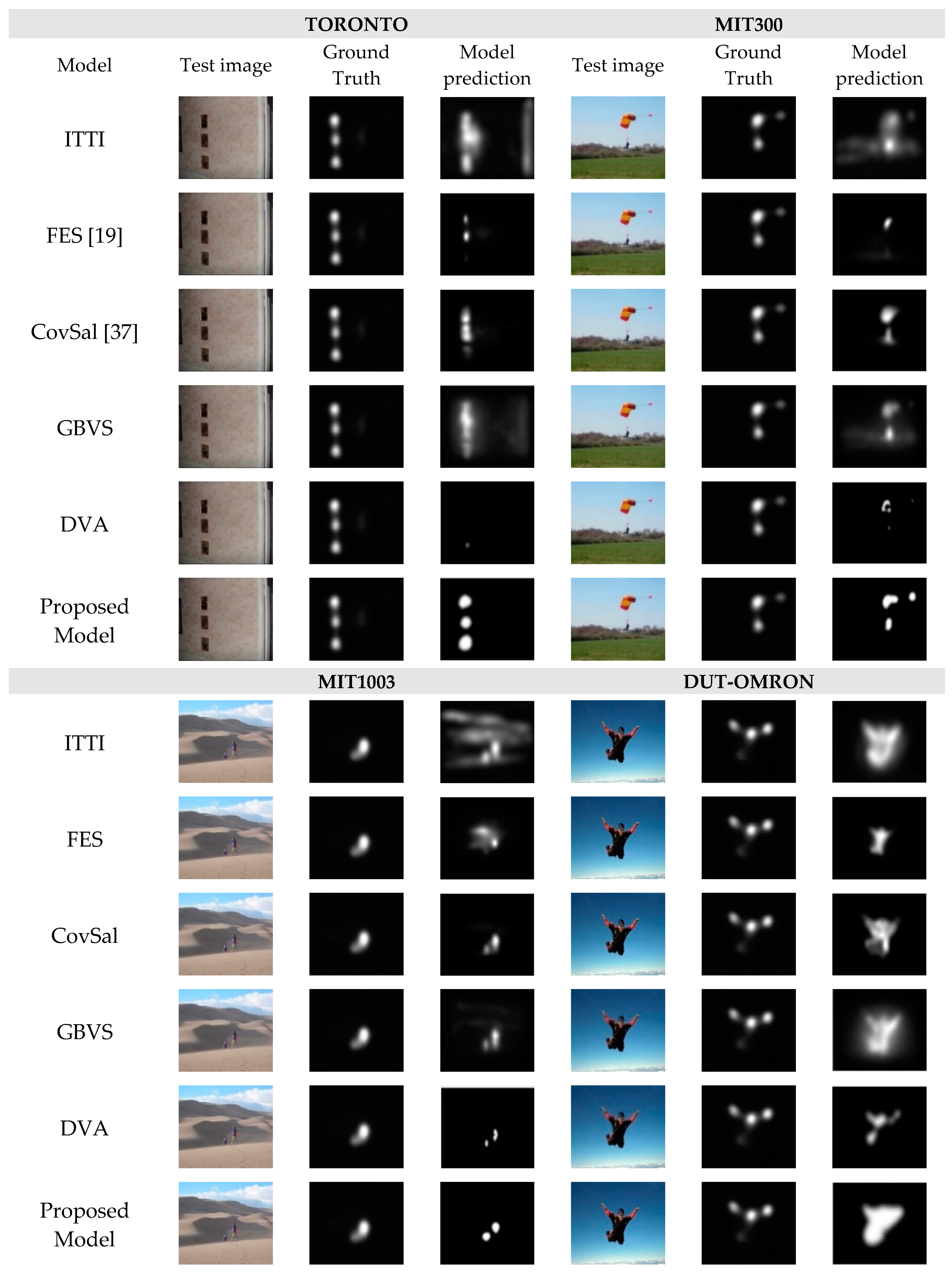
We first qualitatively tested the proposed model with the SALICON dataset; then, we evaluated the model with the TORONTO, MIT300, MIT1003, and DUT-OMRON datasets. Figure 5 illustrates the saliency map results obtained when the proposed model and five other state-of-the-art models are applied to sample images drawn from the studied dataset. From this figure, one can see that the proposed model is capable of predicting most of the salient objects in the given images.
5. Conclusions
In this study, a deep learning model has been proposed to predict visual saliency on images. This work uses a deep network with five encoders and five decoders (convolution and deconvolution) and the semantic segmentation approach to predict human visual saliency. The proposed model generates a sequence of features at the multi-stage level to produce a saliency map. The experimental results obtained from the analysis of four benchmark datasets illustrate the superior prediction capability of the proposed model with respect to other state-of-the-art methods. Additionally, the proposed model achieved an accuracy of more than 94% for all datasets, although the highest performance (i.e., 96%) was obtained with the TORONTO dataset. Additionally, in the training stage, the increased number of training images will increase the prediction accuracy of the proposed model; however, the model requires a larger memory.
In the future, we will focus on how to collect a new dataset, create its ground truth data (e.g., data augmentation method), and design new models with improved evaluation metrics. Importantly, it is possible to use the model presented herein to facilitate other tasks, such as salient object detection, scene classification, and object detection. Moreover, this work provides the basis to develop new models that are able to learn from high-level understanding; for example, they will be able to detect the most interesting part of the image (e.g., a human face) and the most important person in the scene.
Author Contributions
B.G. designed the model, performed the experiments, and wrote the paper, and M.S.S. and P.M. edited the paper.
Acknowledgments
The authors acknowledge the support of the Libyan Ministry of Higher Education and Scientific Research, and Elmergib University, Alkhums.
Conflicts of Interest
The authors declare no conflicts of interest.
References
- Sun, Y.; Fisher, R. Object-based visual attention for computer vision. Artif. Intell. 2003, 146, 77–123. [Google Scholar] [CrossRef] [Green Version]
- Koch, C.; Ullman, S. Shifts in selective visual attention: Towards the underlying neural circuitry. In Matters of Intelligence; Springer: Dordrecht, The Netherlands, 1987; pp. 115–141. [Google Scholar]
- Wang, K.; Wang, S.; Ji, Q. Deep eye fixation map learning for calibration-free eye gaze tracking. In Proceedings of the Ninth Biennial ACM Symposium on Eye Tracking Research & Applications, Charleston, SC, USA, 14–17 March 2016; pp. 47–55. [Google Scholar]
- Borji, A. Boosting bottom-up and top-down visual features for saliency estimation. In Proceedings of the 2012 IEEE Conference on Computer Vision and Pattern Recognition, Providence, RI, USA, 16–21 June 2012; pp. 438–445. [Google Scholar]
- Zhu, W.; Deng, H. Monocular free-head 3D gaze tracking with deep learning and geometry constraints. In Proceedings of the IEEE International Conference on Computer Vision, Venice, Italy, 22–29 October 2017; pp. 3143–3152. [Google Scholar]
- Kanan, C.; Tong, M.H.; Zhang, L.; Cottrell, G.W. SUN: Top-down saliency using natural statistics. Vis. Cogn. 2009, 17, 979–1003. [Google Scholar] [CrossRef] [PubMed] [Green Version]
- Hickson, S.; Dufour, N.; Sud, A.; Kwatra, V.; Essa, I. Eyemotion: Classifying facial expressions in VR using eye-tracking cameras. In Proceedings of the 2019 IEEE Winter Conference on Applications of Computer Vision (WACV), Waikoloa Village, HI, USA, 7–11 January 2019; pp. 1626–1635. [Google Scholar]
- Zhao, R.; Ouyang, W.; Li, H.; Wang, X. Saliency detection by multi-context deep learning. In Proceedings of the IEEE Conference on Computer Vision and Pattern Recognition, Boston, MA, USA, 7–12 June 2015; pp. 1265–1274. [Google Scholar]
- Recasens, A.; Vondrick, C.; Khosla, A.; Torralba, A. Following gaze in video. In Proceedings of the IEEE International Conference on Computer Vision, Venice, Italy, 22–29 October 2017; pp. 1435–1443. [Google Scholar]
- Wang, C.; Shi, F.; Xia, S.; Chai, J. Realtime 3D eye gaze animation using a single RGB camera. ACM Trans. Graph. 2016, 35, 118. [Google Scholar] [CrossRef]
- Cornia, M.; Baraldi, L.; Serra, G.; Cucchiara, R. Paying more attention to saliency: Image captioning with saliency and context attention. ACM Trans. Multimed. Comput. Commun. Appl. 2018, 14, 48. [Google Scholar] [CrossRef]
- Naqvi, R.; Arsalan, M.; Batchuluun, G.; Yoon, H.; Park, K. Deep learning-based gaze detection system for automobile drivers using a NIR camera sensor. Sensors 2018, 18, 456. [Google Scholar] [CrossRef] [PubMed]
- Rezaee, M.; Mahdianpari, M.; Zhang, Y.; Salehi, B. Deep Convolutional Neural Network for Complex Wetland Classification Using Optical Remote Sensing Imagery. IEEE J. Sel. Top. Appl. Earth Obs. Remote Sens. 2018, 11, 3030–3039. [Google Scholar] [CrossRef]
- Krafka, K.; Khosla, A.; Kellnhofer, P.; Kannan, H.; Bhandarkar, S.; Matusik, W.; Torralba, A. Eye tracking for everyone. In Proceedings of the IEEE Conference on Computer Vision and Pattern Recognition, Las Vegas, NV, USA, 26 June–1 July 2016; pp. 2176–2184. [Google Scholar]
- Xu, K.; Ba, J.; Kiros, R.; Cho, K.; Courville, A.; Salakhudinov, R.; Zemel, R.; Bengio, Y. Show, attend and tell: Neural image caption generation with visual attention. In Proceedings of the International Conference on Machine Learning, Lille, France, 6–11 July 2015; pp. 2048–2057. [Google Scholar]
- Kruthiventi, S.S.S.; Gudisa, V.; Dholakiya, J.H.; Venkatesh Babu, R. Saliency unified: A deep architecture for simultaneous eye fixation prediction and salient object segmentation. In Proceedings of the IEEE Conference on Computer Vision and Pattern Recognition, Las Vegas, NV, USA, 26 June–1 July 2016; pp. 5781–5790. [Google Scholar]
- Pan, J.; Sayrol, E.; Giro-i-Nieto, X.; McGuinness, K.; O’Connor, N.E. Shallow and deep convolutional networks for saliency prediction. In Proceedings of the IEEE Conference on Computer Vision and Pattern Recognition, Las Vegas, NV, USA, 26 June–1 July 2016; pp. 598–606. [Google Scholar]
- Mahdianpari, M.; Salehi, B.; Mohammadimanesh, F.; Motagh, M. Random forest wetland classification using ALOS-2 L-band, RADARSAT-2 C-band, and TerraSAR-X imagery. ISPRS J. Photogramm. Remote Sens. 2017, 130, 13–31. [Google Scholar] [CrossRef]
- Liu, N.; Han, J.; Liu, T.; Li, X. Learning to predict eye fixations via multiresolution convolutional neural networks. IEEE Trans. Neural Netw. Learn. Syst. 2016, 29, 392–404. [Google Scholar] [CrossRef] [PubMed]
- Simonyan, K.; Zisserman, A. Very deep convolutional networks for large-scale image recognition. arXiv 2014, arXiv:1409.1556. [Google Scholar]
- Mahdianpari, M.; Salehi, B.; Rezaee, M.; Mohammadimanesh, F.; Zhang, Y. Very deep convolutional neural networks for complex land cover mapping using multispectral remote sensing imagery. Remote Sens. 2018, 10, 1119. [Google Scholar] [CrossRef]
- Jiang, M.; Huang, S.; Duan, J.; Zhao, Q. Salicon: Saliency in context. In Proceedings of the IEEE Conference on Computer Vision and Pattern Recognition, Boston, MA, USA, 7–12 June 2015; pp. 1072–1080. [Google Scholar]
- Judd, T.; Ehinger, K.; Durand, F.; Torralba, A. Learning to predict where humans look. In Proceedings of the 2009 IEEE 12th International Conference on Computer Vision, Kyoto, Japan, 29 September–2 October 2009; pp. 2106–2113. [Google Scholar]
- Bruce, N.; Tsotsos, J. Saliency based on information maximization. In Proceedings of the Advances in Neural Information Processing Systems, Vancouver, BC, Canada, 4–7 December 2006; pp. 155–162. [Google Scholar]
- Li, Y.; Hou, X.; Koch, C.; Rehg, J.M.; Yuille, A.L. The secrets of salient object segmentation. In Proceedings of the IEEE Conference on Computer Vision and Pattern Recognition, Columbus, OH, USA, 23–28 June 2014; pp. 280–287. [Google Scholar]
- Wang, W.; Shen, J. Deep visual attention prediction. IEEE Trans. Image Process. 2017, 27, 2368–2378. [Google Scholar] [CrossRef] [PubMed]
- Mohammadimanesh, F.; Salehi, B.; Mahdianpari, M.; Gill, E.; Molinier, M. A new fully convolutional neural network for semantic segmentation of polarimetric SAR imagery in complex land cover ecosystem. ISPRS J. Photogramm. Remote Sens. 2019, 151, 223–236. [Google Scholar] [CrossRef]
- Krizhevsky, A.; Sutskever, I.; Hinton, G.E. Imagenet classification with deep convolutional neural networks. In Proceedings of the Advances in Neural Information Processing Systems, Lake Tahoe, NV, USA, 3–6 December 2012; pp. 1097–1105. [Google Scholar]
- Long, J.; Shelhamer, E.; Darrell, T. Fully convolutional networks for semantic segmentation. In Proceedings of the IEEE Conference on Computer Vision and Pattern Recognition, Boston, MA, USA, 7–12 June 2015; pp. 3431–3440. [Google Scholar]
- Qian, N. On the momentum term in gradient descent learning algorithms. Neural Netw. 1999, 12, 145–151. [Google Scholar] [CrossRef]
- Judd, T.; Durand, F.; Torralba, A. A Benchmark of Computational Models of Saliency to Predict Human Fixations. 2012. Available online: http://hdl.handle.net/1721.1/68590 (accessed on 9 August 2019).
- Yang, C.; Zhang, L.; Lu, H.; Ruan, X.; Yang, M.-H. Saliency detection via graph-based manifold ranking. In Proceedings of the IEEE Conference on Computer Vision and Pattern Recognition, Portland, OR, USA, 23–28 June 2013; pp. 3166–3173. [Google Scholar]
- Wang, W.; Shen, J.; Yang, R.; Porikli, F. Saliency-aware video object segmentation. IEEE Trans. Pattern Anal. Mach. Intell. 2017, 40, 20–33. [Google Scholar] [CrossRef] [PubMed]
- Harel, J.; Koch, C.; Perona, P. Graph-based visual saliency. In Proceedings of the Advances in Neural Information Processing Systems, Vancouver, BC, Canada, 3–6 December 2007; pp. 545–552. [Google Scholar]
- Borji, A.; Tavakoli, H.R.; Sihite, D.N.; Itti, L. Analysis of scores, datasets, and models in visual saliency prediction. In Proceedings of the IEEE international Conference on Computer Vision, Sydney, Australia, 1–8 December 2013; pp. 921–928. [Google Scholar]
- Tavakoli, H.R.; Rahtu, E.; Heikkilä, J. Fast and efficient saliency detection using sparse sampling and kernel density estimation. In Proceedings of the Scandinavian Conference on Image Analysis, Ystad, Sweden, 23–25 May 2011; pp. 666–675. [Google Scholar]
- Erdem, E.; Erdem, A. Visual saliency estimation by nonlinearly integrating features using region covariances. J. Vis. 2013, 13, 11. [Google Scholar] [CrossRef] [PubMed]
- Bruce, N.D.B.; Tsotsos, J.K. Saliency, attention, and visual search: An information theoretic approach. J. Vis. 2009, 9, 5. [Google Scholar] [CrossRef] [PubMed]
- Csurka, G.; Larlus, D.; Perronnin, F.; Meylan, F. What is a good evaluation measure for semantic segmentation? In Proceedings of the 24th British Machine Vision Conference (BMVC), Bristol, UK, 9–13 September 2013; Volume 27, p. 2013. [Google Scholar]
Figure 1.
General Structure of the VGG-16 network: (a) Convolution layers of the VGG-16 network, and (b) data flow in the VGG-16 network [20].
Figure 1.
General Structure of the VGG-16 network: (a) Convolution layers of the VGG-16 network, and (b) data flow in the VGG-16 network [20].

Figure 2.
Architecture of the proposed model. Note that the size of the input image is explained by (wxh), where w is the width and h is the height. All saliency maps also have a similar size to that of the input image.
Figure 2.
Architecture of the proposed model. Note that the size of the input image is explained by (wxh), where w is the width and h is the height. All saliency maps also have a similar size to that of the input image.

Figure 3.
Value of validation accuracy and loss as a function of epochs.

Figure 4.
Model testing: (a) TORONTO and MIT300 datasets, and (b) MIT1003 and DUT-OMRON datasets.

Figure 5.
The saliency maps obtained from the proposed model and five other state-of-the-art models for a sample image from the TORONTO, MIT300, MIT1003, and DUT-OMRON datasets.
Figure 5.
The saliency maps obtained from the proposed model and five other state-of-the-art models for a sample image from the TORONTO, MIT300, MIT1003, and DUT-OMRON datasets.


Table 1.
Comparison of the quantitative scores of several models for the TORONTO [31] dataset.
Table 1.
Comparison of the quantitative scores of several models for the TORONTO [31] dataset.
| Model | NSS | SIM | AUC-Judd | AUC-Borji |
|---|---|---|---|---|
| ITTI [38] | 1.30 | 0.45 | 0.80 | 0.80 |
| AIM [23] | 0.84 | 0.36 | 0.76 | 0.75 |
| Judd Model [34] | 1.15 | 0.40 | 0.78 | 0.77 |
| GBVS [31] | 1.52 | 0.49 | 0.83 | 0.83 |
| Mr-CNN [39] | 1.41 | 0.47 | 0.80 | 0.79 |
| DVA [26] | 2.12 | 0.58 | 0.86 | 0.86 |
| Proposed Model | 3.00 | 0.42 | 0.91 | 0.87 |
Note: Humans baseline [29] 3.29 1.00 0.92 0.88.
Table 2.
Comparison of the quantitative scores of several models for the MIT300 [31] dataset.
Table 2.
Comparison of the quantitative scores of several models for the MIT300 [31] dataset.
| Model | NSS | SIM | AUC-Judd | AUC-Borji |
|---|---|---|---|---|
| ITTI | 0.97 | 0.44 | 0.75 | 0.74 |
| AIM | 0.79 | 0.40 | 0.77 | 0.75 |
| Judd Model | 1.18 | 0.42 | 0.81 | 0.80 |
| GBVS | 1.24 | 0.48 | 0.81 | 0.80 |
| Mr-CNN | 1.13 | 0.45 | 0.77 | 0.76 |
| DVA | 1.98 | 0.58 | 0.85 | 0.78 |
| Proposed Model | 2.43 | 0.51 | 0.87 | 0.80 |
Table 3.
Comparison of the quantitative scores of several models for the MIT1003 [31] dataset.
Table 3.
Comparison of the quantitative scores of several models for the MIT1003 [31] dataset.
| Model | NSS | SIM | AUC-Judd | AUC-Borji |
|---|---|---|---|---|
| ITTI | 1.10 | 0.32 | 0.77 | 0.76 |
| AIM | 0.82 | 0.27 | 0.79 | 0.76 |
| Judd Model | 1.18 | 0.42 | 0.81 | 0.80 |
| GBVS | 1.38 | 0.36 | 0.83 | 0.81 |
| Mr-CNN | 1.36 | 0.35 | 0.80 | 0.77 |
| DVA | 2.38 | 0.50 | 0.87 | 0.85 |
| Proposed Model | 2.39 | 0.42 | 0.87 | 0.80 |
Table 4.
Comparison of the quantitative scores of several models for the DUT-OMRON [31] dataset.
Table 4.
Comparison of the quantitative scores of several models for the DUT-OMRON [31] dataset.
| Model | NSS | SIM | AUC-Judd | AUC-Borji |
|---|---|---|---|---|
| ITTI | 3.09 | 0.53 | 0.83 | 0.83 |
| AIM | 1.05 | 0.32 | 0.77 | 0.75 |
| GBVS | 1.71 | 0.43 | 0.87 | 0.85 |
| DVA | 3.09 | 0.53 | 0.91 | 0.86 |
| Proposed Model | 2.50 | 0.49 | 0.91 | 0.84 |
Table 5.
Model predication results (i.e., global accuracy) for several datasets (TORONTO, MIT300, MIT1003, and DUT-OMRON).
Table 5.
Model predication results (i.e., global accuracy) for several datasets (TORONTO, MIT300, MIT1003, and DUT-OMRON).
| Datasets | Global Accuracy | WeightedIoU |
|---|---|---|
| TORONTO | 0.96227 | 0.94375 |
| MIT300 | 0.94131 | 0.91924 |
| MIT1003 | 0.94862 | 0.92638 |
| DUT-OMRON | 0.94484 | 0.92605 |
© 2019 by the authors. Licensee MDPI, Basel, Switzerland. This article is an open access article distributed under the terms and conditions of the Creative Commons Attribution (CC BY) license (http://creativecommons.org/licenses/by/4.0/).
Share and Cite
MDPI and ACS Style
Ghariba, B.; Shehata, M.S.; McGuire, P. Visual Saliency Prediction Based on Deep Learning. Information 2019, 10, 257. https://doi.org/10.3390/info10080257
AMA Style
Ghariba B, Shehata MS, McGuire P. Visual Saliency Prediction Based on Deep Learning. Information. 2019; 10(8):257. https://doi.org/10.3390/info10080257
Chicago/Turabian StyleGhariba, Bashir, Mohamed S. Shehata, and Peter McGuire. 2019. "Visual Saliency Prediction Based on Deep Learning" Information 10, no. 8: 257. https://doi.org/10.3390/info10080257
Note that from the first issue of 2016, this journal uses article numbers instead of page numbers. See further details here.