Article

Hadoop Performance Analysis Model with Deep Data Locality †

1
Department of Computer Science, University of Wisconsin-Whitewater; Whitewater, WI 53190, USA
2
Department of Computer Science, University of Nevada, Las Vegas, NV 89154, USA
*
Author to whom correspondence should be addressed.
This paper is an extended version of our presentation in the 2018 IEEE International Conference on Big Data, Seattle, WA, USA, 10–13 December 2018.
Information 2019, 10(7), 222; https://doi.org/10.3390/info10070222
Submission received: 11 June 2019 / Revised: 23 June 2019 / Accepted: 26 June 2019 / Published: 27 June 2019
(This article belongs to the Special Issue Big Data Research, Development, and Applications––Big Data 2018)

Abstract

:
Background: Hadoop has become the base framework on the big data system via the simple concept that moving computation is cheaper than moving data. Hadoop increases a data locality in the Hadoop Distributed File System (HDFS) to improve the performance of the system. The network traffic among nodes in the big data system is reduced by increasing a data-local on the machine. Traditional research increased the data-local on one of the MapReduce stages to increase the Hadoop performance. However, there is currently no mathematical performance model for the data locality on the Hadoop. Methods: This study made the Hadoop performance analysis model with data locality for analyzing the entire process of MapReduce. In this paper, the data locality concept on the map stage and shuffle stage was explained. Also, this research showed how to apply the Hadoop performance analysis model to increase the performance of the Hadoop system by making the deep data locality. Results: This research proved the deep data locality for increasing performance of Hadoop via three tests, such as, a simulation base test, a cloud test and a physical test. According to the test, the authors improved the Hadoop system by over 34% by using the deep data locality. Conclusions: The deep data locality improved the Hadoop performance by reducing the data movement in HDFS.

1. Introduction

Nowadays, the volume of data is growing exponentially in a similar way to Moore’s law. According to IDC [1], the global data volume is growing twice every two years. The need for more efficient big data analytics is growing accordingly. Apache Hadoop [2] has become a fundamental framework to process such big data. Hadoop follows a simple principle of “moving computation is cheaper than moving data” [2]. In a traditional data processing system, the target data is moved to the server for processing, but it creates a bottleneck of data transfer. For example, copying 1 TB of data on a hard drive with a typical speed of 100 MB/s takes almost 3 h. Even if the data is divided into 100 hard drives, copying 10 GB to a target server still takes 100 s. Hadoop solves this bottleneck by sending the code to the server where the target data resides as much as possible, thereby reducing or removing the data transfer overhead. This concept is called data locality and it affects the Hadoop performance greatly. As a result, researchers have been trying to increase data locality via various methods such as scheduling, system configuration, cluster management, etc. However, there has been a critical missing link. When executing MapReduce (MR) on Hadoop, the data locality can be applied only to the initial stage in all schemes, and therefore there is a severe limitation in improving the performance. It would be desirable if high data locality can be maintained throughout the entire MR stages.
The authors explored a novel concept of deep data locality (DDL) that extends the benefit of data locality to all stages of MR. The research has found that under certain conditions, the DDL method can improve MR performance by over 34%. This improvement is enormous in that it could change the Hadoop processing paradigm in the future. This study developed the computation model for analyzing Hadoop performance under various conditions and an associated simulator to demonstrate the effects of the conditions. A preliminary experiment with a small hardware testbed was also conducted to compare the performance of DDL with conventional mechanisms.
In this research, the analytical model was explained to generalize the Hadoop processing performance in Section 3, and tested it via three tests, such as, a simulation-based test, a cloud-based test and a realistic hardware testbed, in Section 5. In Section 2, the background of the Hadoop system and data locality was explained with literature reviews. The authors illustrated the deep data concept and methods, such as block-based DDL and key-based DDL, to apply the Hadoop performance analysis model on the Hadoop system, in Section 4. Section 6 discusses conclusions and future work.

2. Overview of Hadoop and Data Locality with Literature Reviews

2.1. Hadoop System

Hadoop is a distributed system that utilizes low-cost commodity hardware systems. Input data is split into blocks and distributed into multiple nodes. Hadoop has a master-slave architecture and the Node Manager in slave nodes communicates with the master node by sending a heartbeat message. Master node distributes the job to slave nodes to process large-scale data based on the metadata and heartbeats messages. Hadoop has four major modules, that is, Hadoop common, yet another resource negotiator (YARN), Hadoop Distributed File System (HDFS), and MR. Hadoop common has common utilities for Hadoop configuration, libraries, and support functions for other modules. YARN performs cluster resource management such as managing slave nodes’ resources, scheduling task and monitoring the data nodes using the scheduler and application manager [3]. Many different processing engines, such as Storm [4], Spark [5] HBase [6], or RHadoop [7] can operate simultaneously across a Hadoop cluster and some analysis tools such as R, Matlab [8], SAS, or SPSS can work on Hadoop over YARN. HDFS is a distributed storage system where the master node manages the location of real data blocks in slave nodes. HDFS is the primary of the data locality and is discussed later. MR is a software framework to process large-scale data in parallel on large clusters [9]. MR can be used by itself or with other analysis tools (e.g., R, Matlab, SAS, or SPSS) through an application program interface (API).
MR is a technique for processing very large datasets simultaneously over many cores. First, the scheduler creates several containers in the slave nodes to divide the job into several tasks. A container is a YARN Java virtual machine process associated with a collection of physical resources including CPU core, disk and memory. There has been considerable research on the scheduling to optimize the usage of resources in the slave nodes using container allocation [10], data locality [10,11], storage [11], optimizing configuration of Hadoop [12], and workload balancing [13]. Each node has a single node manager, which reports the status of the node, such as CPU, memory, and disk status, to the resource manager using heartbeat. The scheduler makes the job scheduling based on the information of the heartbeat [14], and the heartbeat has an influence on the initialization and the termination of a job [15].
The MR process on Hadoop can be broken into small stages as shown in Figure 1. The map step reads input data and emits key/value pairs, which is called a partition. Then, the shuffle step redistributes the data to the reduce nodes based on the output of the map. Further, the reduce step combines a list of values into a smaller number of values. The data locality concepts in this research are described in further detail.
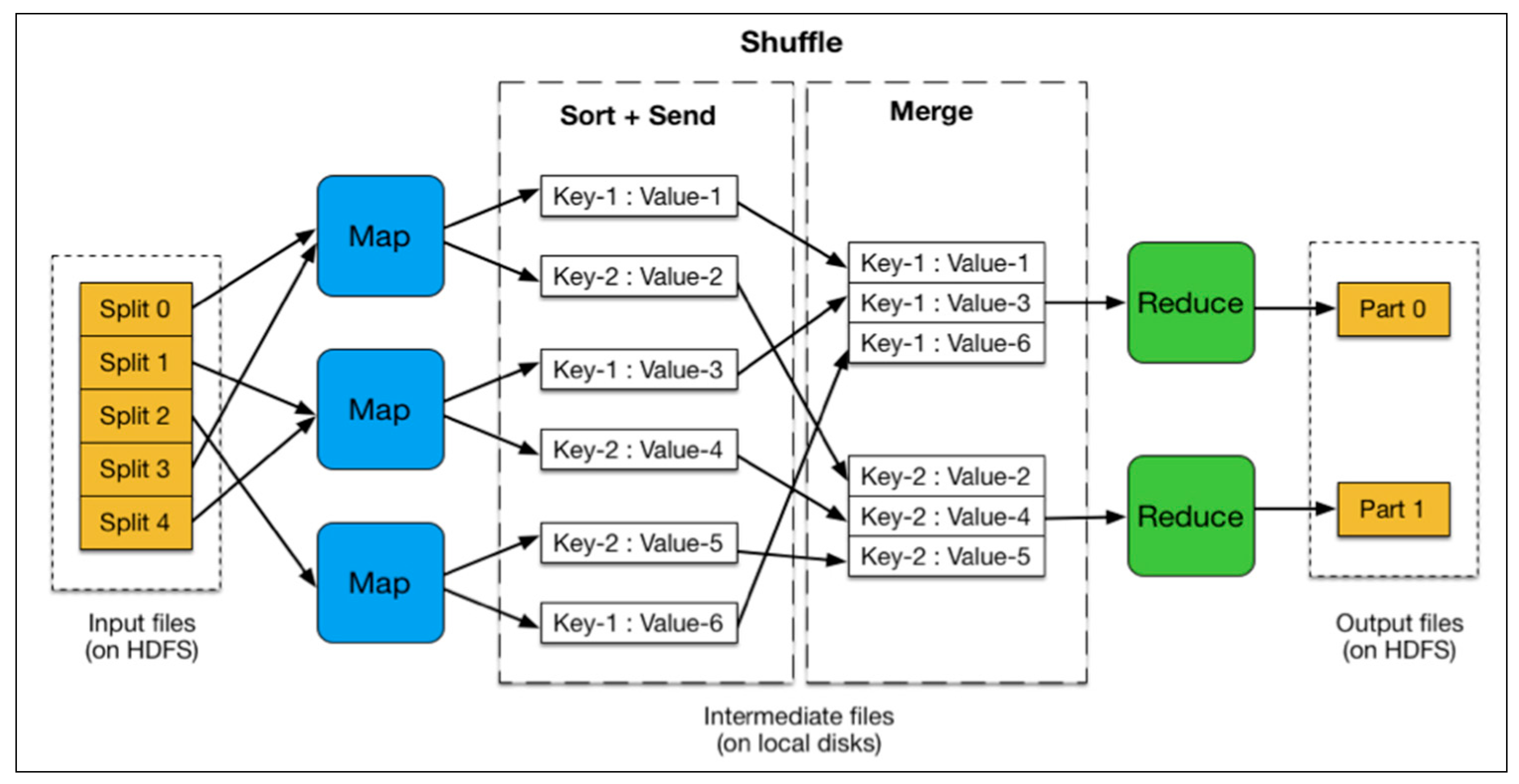
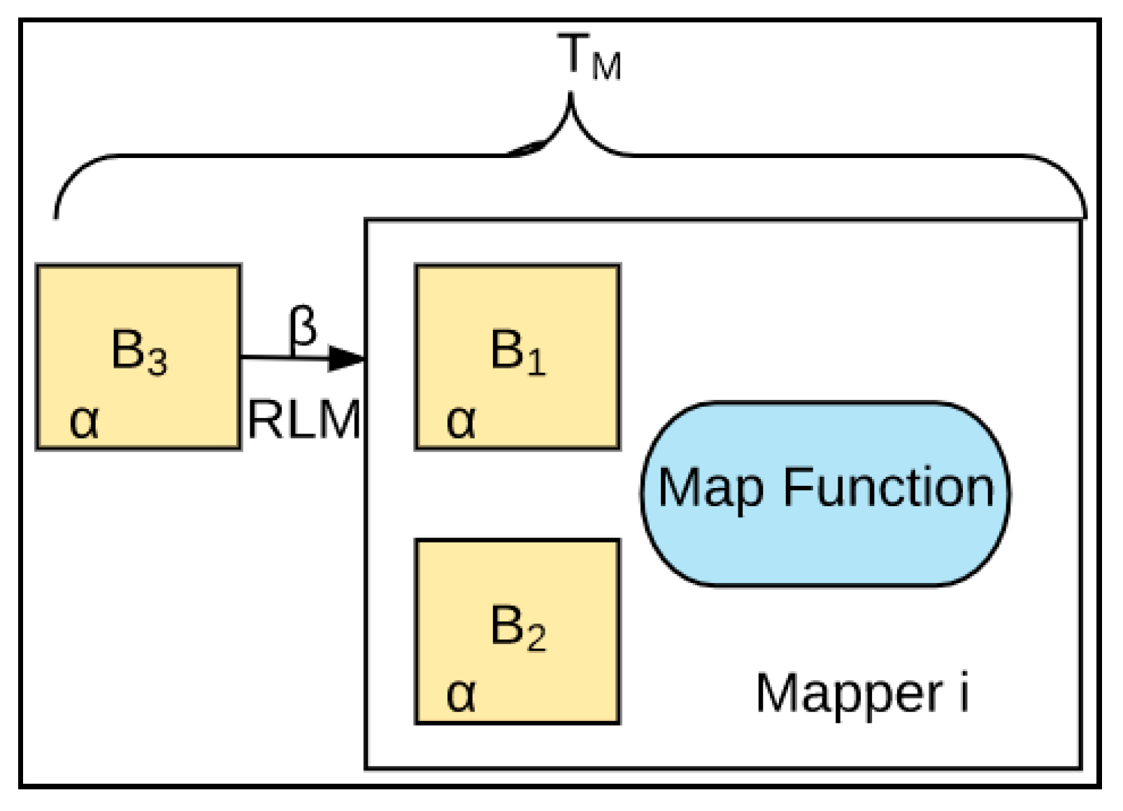
  • Map: Mappers in containers execute the task using the data block in slave nodes. This is a part of the actual data manipulation for the job requested by the client. All mappers in the containers execute the tasks in parallel. The performance of the mapper depends on scheduling [10,12], data locality [16,17], programmer skills, container’s resources, data size and data complexity.
  • Sort/Spill: The output pair which is emitted by the mapper is called partition. The partition is stored and sorted in the key/value buffer in the memory to process the batch job. The size of the buffer is configured by resource tracker and when its limit is reached, the spill is started.
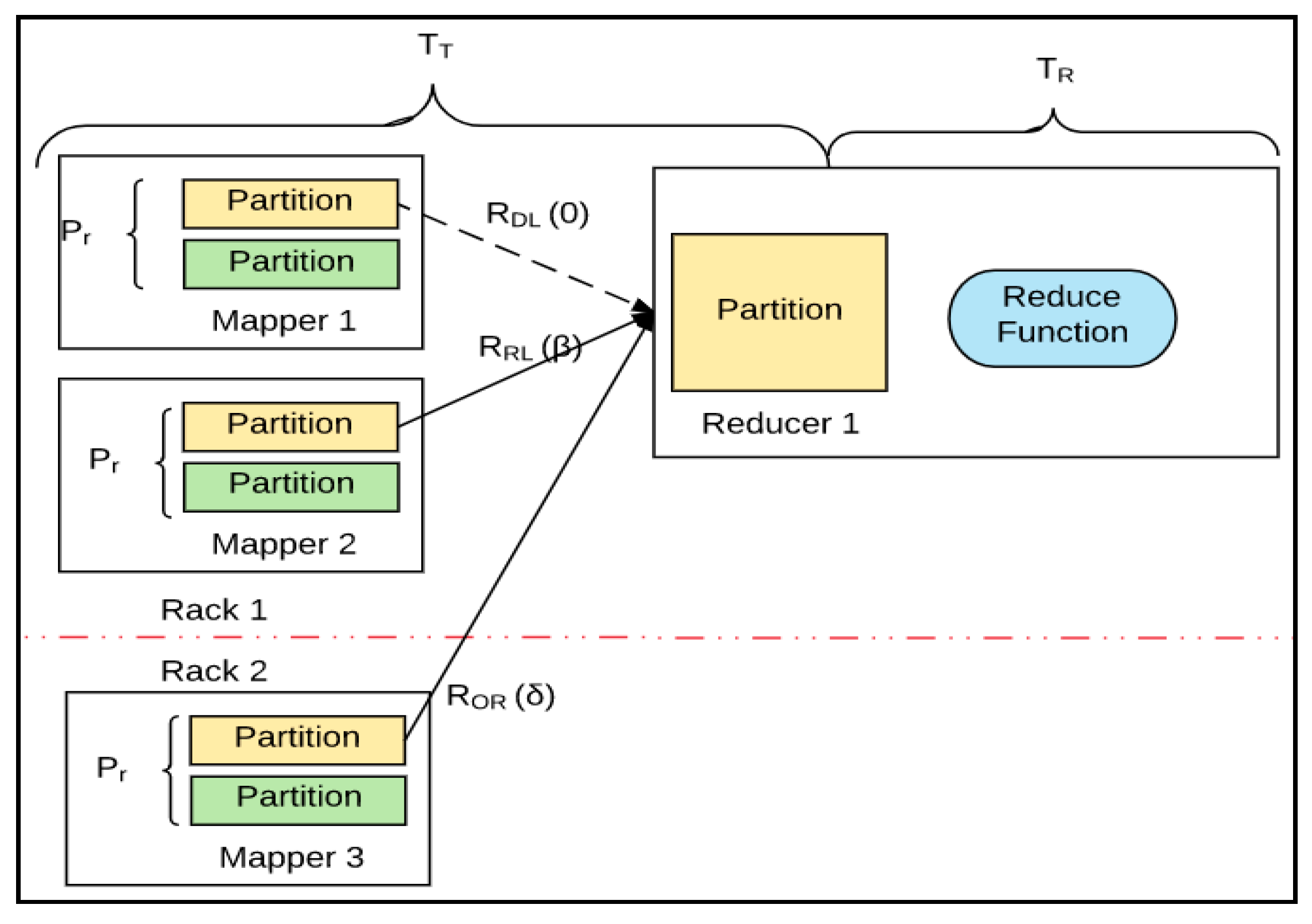
  • Shuffle: The key/value pairs in the spilled partition are sent to the reduce nodes based on the key via the network in this step. To increase the network performance, researchers have approached it from software defined network (SDN) [18], remote direct memory access (RDMA) [19], and Hadoop configurations [20], etc.
  • Merge: The partitions in the partition set are merged to finish the job. This step has usually been studied along with the shuffle step, such as in-memory with compression [21,22].
  • Reduce: The slave nodes process the merged partition set to make a result of the application. The performance of reduce depends on scheduling [10,12], locality [16,17], programmer skills, container resources, data size, and data complexity, as was the case in the map step. However, unlike in the map step, the reduce step can be improved by in-memory computing [5,21,22,23].
  • Output: The output of reduce nodes is stored at HDFS on the slave nodes.

2.2. Hadoop Locality Research

The research on Hadoop data locality was approached from multiple aspects. Hadoop framework is broken down to Figure 2 to show the stages in each layer and related research. Most research focused on YARN and MR layers, and the underlying HDFS layer was rarely touched. Without optimizing the HDFS layer, the overall performance is very limited. Also, they tend to focus on the early stage (e.g., Map). Our research, however, is focused on the HDFS layer and it affects the layers above it. It also works throughout all 3 stages.

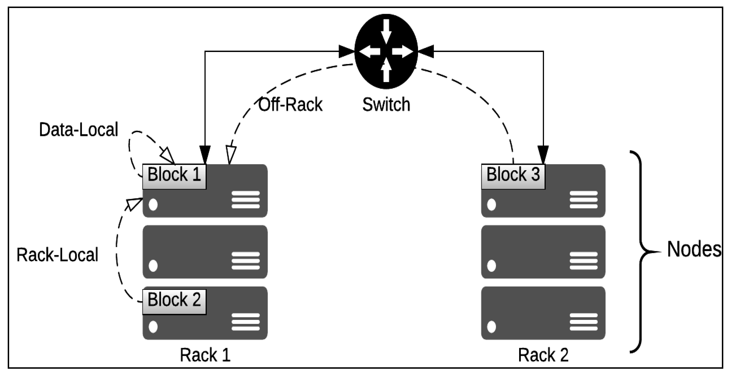
2.3. Hadoop Data Locality in Map Stage

Data locality policy allows a map program to be executed on the same node where the data is located in order to reduce network traffic. During this process, to increase the data locality and fault-tolerance, Hadoop makes several replicas of data blocks, and distributes them to multiple slave nodes. The data blocks may be located in any of the following three locations, in the order of decreased locality like Figure 3.
There are three data locality such as:
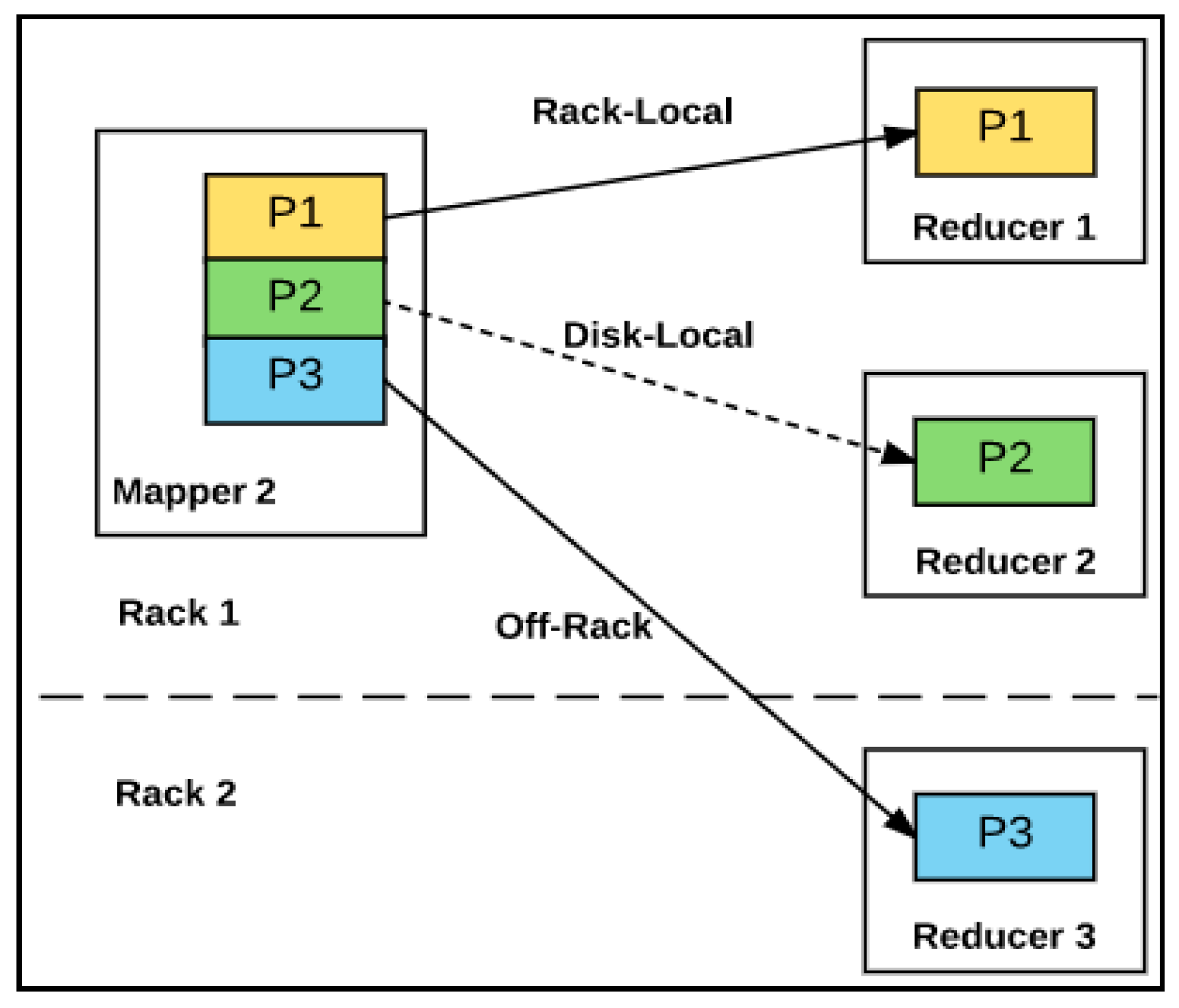
  • Local disk (data-local map): The data block is on the local disk.
  • In-rack disk (rack-local map): The data block is on another node on the same rack.
  • Off-rack disk: The data block is not on the same rack, but another rack.
In an ideal situation, all blocks should be data-local map and there should not be any data transfer between slave nodes. However, under the default HDFS block placement algorithm [24], blocks are randomly distributed to the slave nodes and the slave nodes may be asked to process the blocks they do not have. Then, they need to get the absent blocks from other nodes, resulting in rack-local map (RLM). Since different blocks are assigned to slave nodes in every execution, each execution generates a different number of RLM blocks. Obviously, the more RLM blocks there are, the lower the performance.
When there are a large number of data blocks and computing nodes, the inefficiency on block assignment is also greater, and Hadoop will attempt to utilize the computing nodes even when the data block is not locally present. Therefore the number of RLMs also increases as the number of blocks increases, causing lower performance [25].
There are several methods to reduce RLM blocks. If Hadoop creates more replicas in slave nodes, the data locality will increase, but the storage cost also increases. Therefore, researchers have tried to optimize the number of replicas and block placement in slave nodes using improved locality [12,17], scheduling [12], etc. The research on hardware uses in-memory data processing, such as Apache Storm in Hadoop [4], Apache Spark on Hadoop [5], MapR on Shark [26]. However, they result in a higher memory cost, and are limited in handling the middle output that can grow quite large.

2.4. Hadoop Data Locality beyond Map Stage

Even if the data locality is accomplished perfectly without any RLM in the map stage, the resulting data should be transferred to reducers inevitably during shuffle stage. Therefore, the benefit of data locality is limited to the map stage. In reality, the overhead of shuffle is very high. For example, consider a Hadoop system consisting of 8 slave nodes and each sending 100 blocks of 128 MB to other nodes. In this case, the total data size is fairly small, i.e., only about 100 GB (= 8 nodes × 100 blocks × 128 MB), not even big data. Over 1 Gbps ethernet, transmitting one block takes about 1 s per 128 MB block. Each node needs to send 7/8 of the 100 blocks (= 87.5 blocks) to other reducer nodes, so the shuffle stage will take almost 87.5 s. Even a slight reduction of the shuffle time can bring a great benefit to big data processing, but unfortunately, this aspect has rarely been studied.

2.5. Proposed Approach

This study has developed a novel method to extend the locality to all stages of MR, and minimize the overhead of the shuffle. The authors call it deep data locality (DDL) as opposed to the traditional map-only locality that the authors call shallow data locality (SDL) [25]. Furthermore, this study investigated two different types of DDL methods. First, the block-based DDL reduces the RLM and reduces the data transfer in multicore processors [27]. In multicore processors, all the cores share the same local disk, therefore there is no data transfer overhead between the cores. Second, key-based DDL pre-arranges the data elements in the input data by their key so that only the data elements destined to a certain reducer are assigned to the same mapper [28]. As a result, data transfer does not occur. The pre-arrangement of the data elements can be performed before the map stage, i.e., ETL stage. The relationship between SDL, block-based DDL and key-based DDL is illustrated in Figure 4. The detail of block-based DDL and key-based DDL has been explained in Section 4. Before moving to the DDL methods, an analysis of the Hadoop performance in Section 3 was undertaken.

3. Analyzing Hadoop Performance

How important is data locality and how much improvement can DDL bring in? To answer it, the authors developed a Hadoop performance analysis model. This model is divided into two stages: (1) Map function and sort/spill/fetch, processed by the mapper; and (2) transfer and reduce function, processed by the reducer. Table 1 and Table 2 summarize the notations used in this model. Figure 5 illustrates the related stages for the time variables.

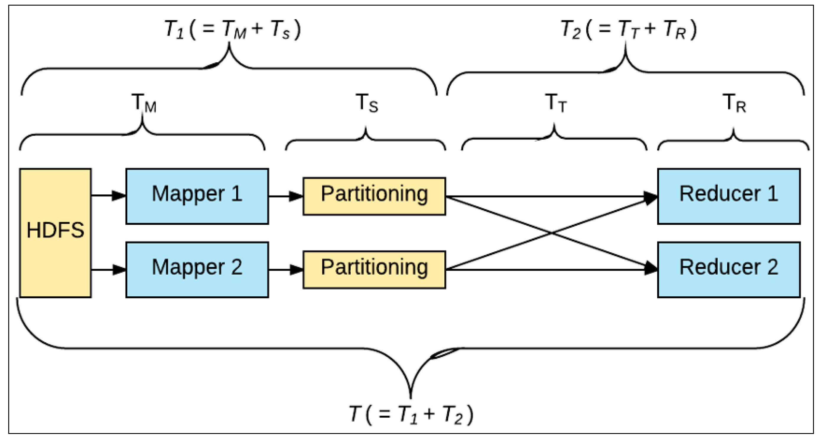
3.1. First Stage (T1)

All mappers work in parallel to make partitions from the allocated blocks. The resulting partitions go through sort/spill and fetch. There are two data localities at this stage, i.e., data-local and rack-local. The processing time of each block takes the same time (α) in mapper (i). transferring each block (b) takes the same time (β). Therefore:
T M   ( i ,   b ) = { α , ( I f   b l o c k   i s   i n   t h e   N o d e ) α + β ,   ( I f   b l o c k   n o t     i n   t h e   N o d e )  
Figure 6 shows the map function time in mapper (i). The processing time of map function (TM) depends on the number of allocated blocks and the number of RLM:
T M   ( i ) = { | B i |   α   +   R L M i     β }
The processing time of sort/spill and fetch on each mapper can be calculated by multiplying the number of allocated blocks and processing time of sort, spill and fetch for one block ( γ ):
T S ( i ) = ( | B i | γ )
The processing time of the first stage on each mapper can be calculated by adding the above two processing times as shown in Figure 7:
T 1 ( i ) = T M   ( i ) + T S ( i )
The longest processing time among all mappers is the processing time of the first stage (T1):
T 1 = m a x 1 i M   { T M   ( i )   +   T S ( i ) } = m a x 1 i M { | B i |   α + R L M i     β + ( | B i | γ ) } = m a x 1 i M { | B i | ( α + γ ) + R L M i     β }
Figure 8 shows the effect of RLM in this model. The more RLM blocks there are, the longer the processing time becomes.

3.2. Second Stage (T2)

This stage includes two processing times, that is, the transfer time (TT) between the mapper and reducer, and the processing time of the reducer function (TR) like Figure 9.
To get them, the middle output size on the reducer (j) needs to be known. The middle output size on the reducer can be calculated by the partitions in the mappers because each mapper is supposed to send the partition to the reducer. The middle output size of the reducer is the total number of block multiplied by the partition ratio per block:
P r ( j ) i = 1 M | B i |
In the second stage, there are three data locality types, i.e., data-local, rack-local and off-rack (Figure 10).
Each partition on the mapper has one of those locality types. For example, if the partition is supposed to stay in the same node, it is data-local (Figure 3). If the partition is supposed to be transferred to a different node in the same rack, it is rack-local, otherwise, it is off-rack (Figure 3). Using the transfer time of one block under rack-local (β) and off-rack (δ), the network transfer time between mappers and reducer (TT) can be calculated as:
T T ( j ) = P r ( j ) i = 1 M | B i | { 0 R D L   ( j ) + β R R L ( j ) + δ R O R ( j ) } = P r ( j ) i = 1 M | B i |   { β     R R L ( j ) + δ     R O R ( j ) }
The transfer time (TT) under data-local is 0 because the partition is already in the reducer. The processing time of the reducer function depends on the size of the middle output. Therefore, the processing time of the reduce function is the size of middle output on the reducer multiplied by the processing time for one block (α):
T R ( j ) = P r ( j ) i = 1 N ( | B i | α )
By adding the processing time of the transfer time to the reducer TT(j) and the processing time on the reducer TR(j), the processing time of the second stage on the reducer T2 was calculated. It is the longest processing time among the reducers, which is equal to the max value among the transfer time plus the processing time of the reducer function:
T 2 = m a x 1 j R { T T ( j ) + T R ( j ) } = m a x 1 j R { P r ( j ) i = 1 N | B i | { β     R R L ( j ) + δ     R O R ( j ) } + P r ( j ) i = 1 N ( | B i | α ) } = m a x 1 j R [ P r ( j ) i = 1 N | B i | { α + β     R R L ( j ) + δ     R O R ( j ) } ]
Figure 11 shows the second stage processing time under the different rack-local and off-rack ratio. As the ratio of either rack-local or off-rack grows, the processing time increases especially as the off-rack blocks have a greater impact in increasing the processing time.

3.3. Total Hadoop Processing Time (T)

The total Hadoop processing time can be obtained by adding two stages:
T = T 1 + T 2 = m a x 1 i M   { | B i | ( α + γ ) + R L M i   β } + m a x 1 j R [ P r ( j ) i = 1 N | B i | { α + β     R R L ( j ) + δ     R O R ( j ) } ]
Figure 12 shows the graph of total Hadoop processing time. Rack local map (RLM) in the first stage, and rack-local (RRL) and off-rack (ROR) in the second stage are the locality types that negatively affect the Hadoop performance. Compared with the ideal case where the data local is 100% in both stages, when the RLM is 100% in the first stage and the rack-local is 100% in the second stage, total Hadoop processing time is twice larger. Furthermore, if the second stage has 100% off-rack data, the total Hadoop processing time is three times larger than the case of data-local only. This observation gives an important insight in data locality. DDL minimizes the RLM on the first stage and maximizes the data-local on the second stage, thereby increasing the performance of Hadoop.

4. Deep Data Locality

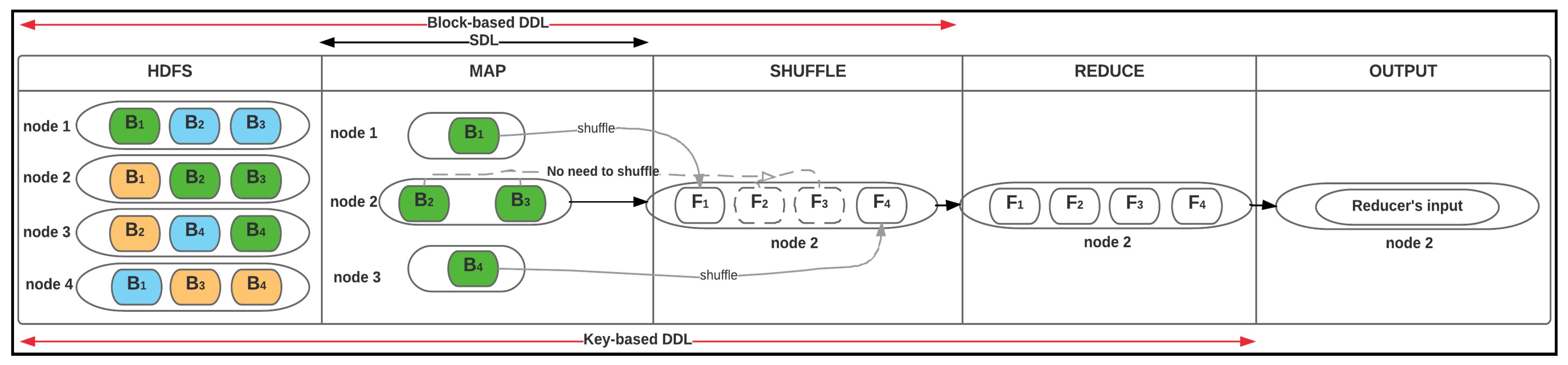
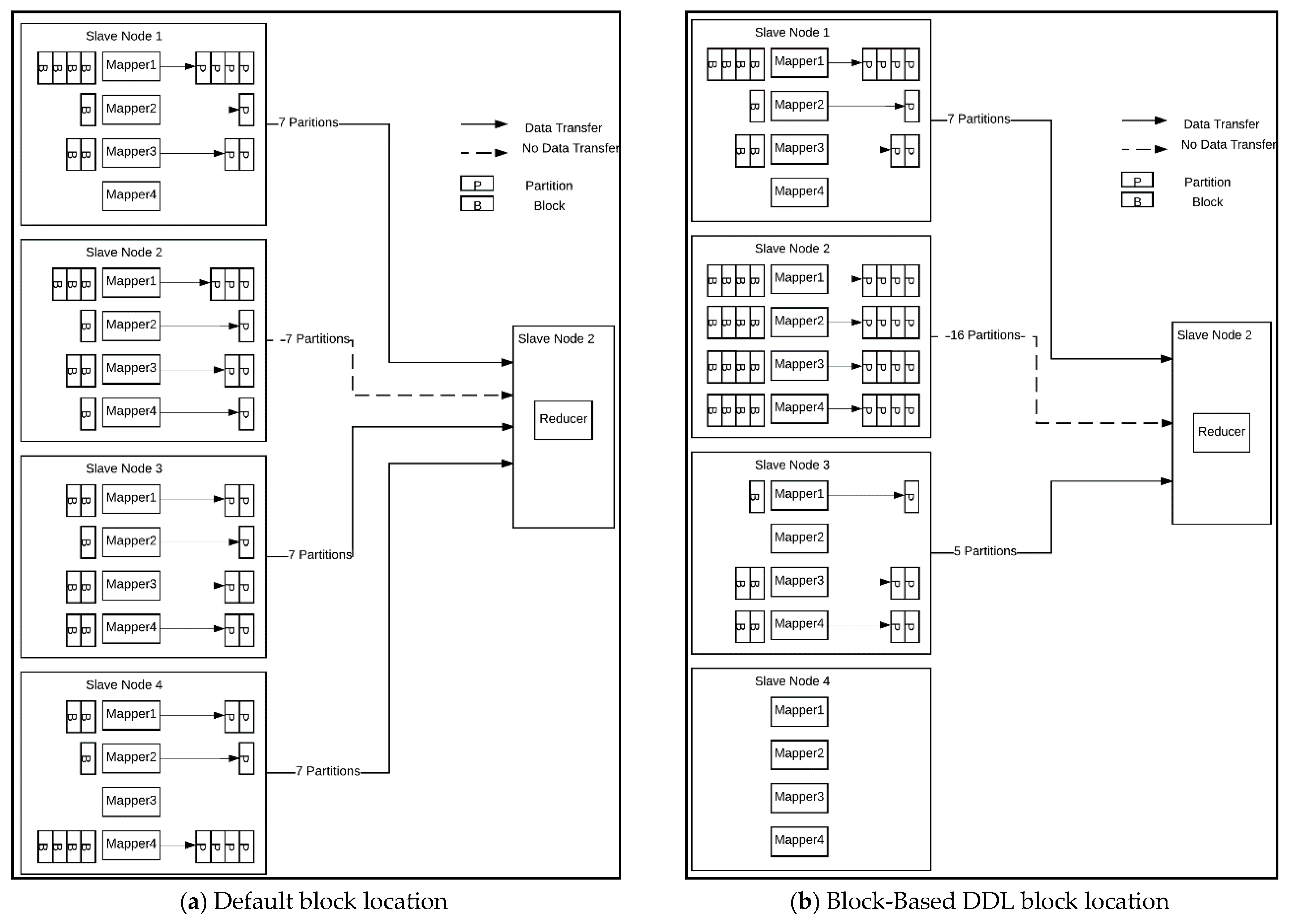
4.1. Block-Based DDL
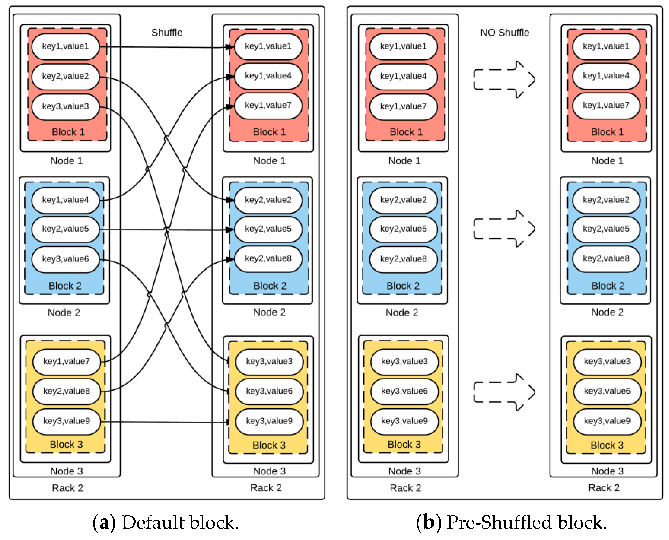
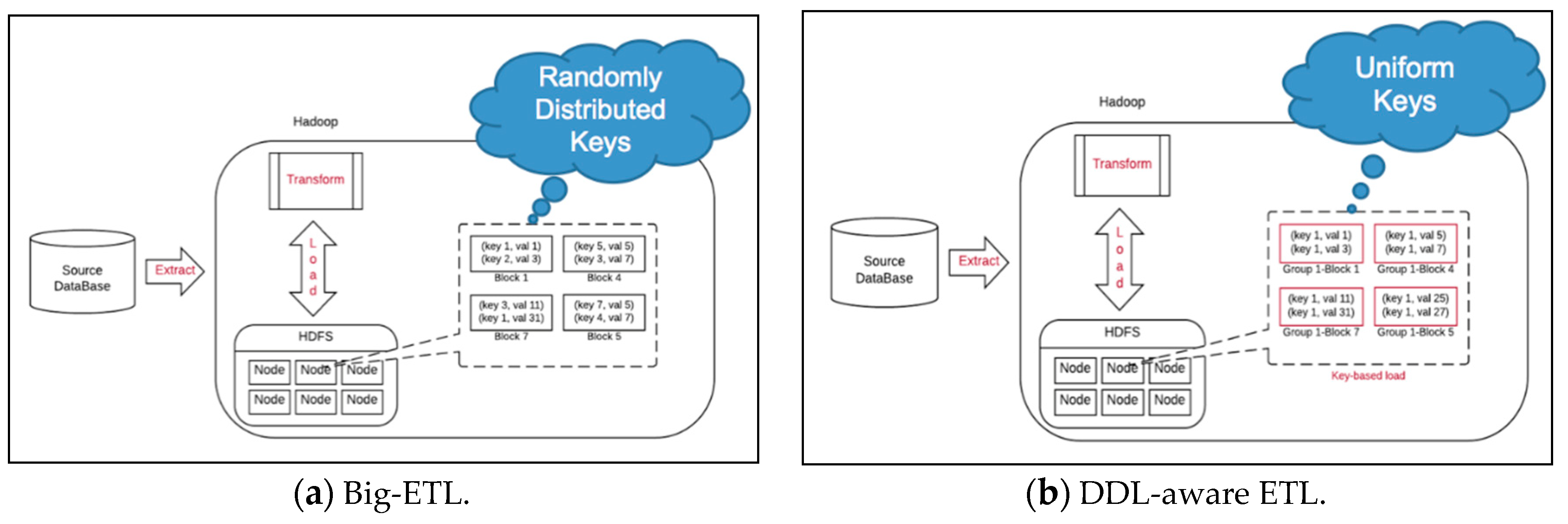
The key idea in block-based is replicating data blocks to the mapper nodes that would become reducer nodes [8]. This would reduce the data transfer during shuffle. This concept is illustrated in Figure 13.
There are two active jobs with different sets of blocks. With the default policy shown in Figure 13a, the containers are evenly distributed for load balancing. In this case, any node could become a reduce node after finishing the map. The node that becomes a reduce node must collect the output from other map nodes. For example, if one of the containers in the node 1 performs a reduce work, the map output from nodes 2, 3 and 4 must be sent to node 1. However, in block-based DDL in Figure 13b, the data blocks are consolidated to a smaller number of nodes (nodes 1 and 2). It then selects node 1 as a reduce node for job 1 and node 2 for job 2. As a result, only the output from node 3 needs to be sent to node 1 for job 1, and the output from node 4 is sent to node 2 for job 2. This significantly reduced the shuffle traffic.
Block-based DDL also utilizes multicore computing. It consolidates the mapper jobs in a small number of nodes so that a smaller number of replicas can be shared by a larger number of cores. This reduces the number of replicas and the storage requirements.

4.2. Key-Based DDL

In MR, after finishing a map job, mapper nodes become reducer nodes. Meanwhile, the mapper nodes send the partition that they have created to an appropriate reducer. If a reducer has an appropriate partition already, it does not need to send it to any other nodes. In an extreme case, if every reducer has only the appropriate partition for itself, no node needs to send any data to other nodes. This is the concept of key-based DDL [29]. This is illustrated in Figure 14.
This is possible only when the input block at the map stage already has the data elements only for this particular reducer. Therefore, it is necessary to pre-process the input blocks before MR. To achieve this, this study proposed using ETL (extract, transform and load) operation which must be done in most big data operations. ETL is a process of pulling data out of the source systems and placing it into a data warehouse. Through ETL, data is extracted from external data sources, converted to proper format, and loaded in the final target. For example, duplicate data gets removed, columns many be combined or transformed, or invalid data gets rejected. In fact, ETL can be done cost-effectively by Hadoop and many commercial or open source products already exist including, InfoSphere by IBM [30], Data Integrator by Oracle [31], PowerCenter by Informatica [32], TeraStream by DataStreams [33], DataStage, Hadoop-ELT, or Hadoop-ETLT. These products are called big-ETL and the authors plan to add one more step to big-ETL. In big-ETL, the data gets aggregated, sorted, transformed and analyzed inside Hadoop. This study proposes adding one more step to big-ETL, i.e., creating files with different keys. Figure 15 shows the difference between big-ETL and DDL-aware ETL. In big-ETL, the input blocks have random keys, but in DDL-aware ETL, the blocks have homogeneous keys. These input blocks can be fed to MR and achieve key-based DDL. This is illustrated in Figure 15.

5. Performance Testing

The performance of Hadoop in three different environments was tested to compare DDL and traditional data locality. First, this study experimented with the block-based DDL and default Hadoop policy on Cloudlab. Second, a simulator to study a variety of conditions was developed based on the Hadoop performance model. Third, a small testbed in hardware was used to collect experimental data.

5.1. Hadoop Performance Test on Cloud

The authors executed Terasort Benchmark program on a Hadoop system composed of 10 slave nodes configured on CloudLab [34]. Each node was equipped with 6 GB memory, 2 Xeon E5-2650v2 processors (8 cores each, 2.6 GHz) and 1 TB hard drive. Hadoop 2.7.1 was installed on Ubuntu 14. Three different data sets have been created by Teragen, i.e., two 30 GB data, two 60 GB data, and two 120 GB data. The test was executed 10 times and the results were averaged. Table 3 shows the results. It shows a significant time reduction in shuffle under block-based DDL (LNBPP) ranging from 18% to 30%.
Some performance improvement was also observed in the map due to the elimination of RLM. The decreasing time was by 9% to 17.7% by block-based DDL in total. This result is rather counterintuitive because it may look better to distribute the job to as many nodes as possible.

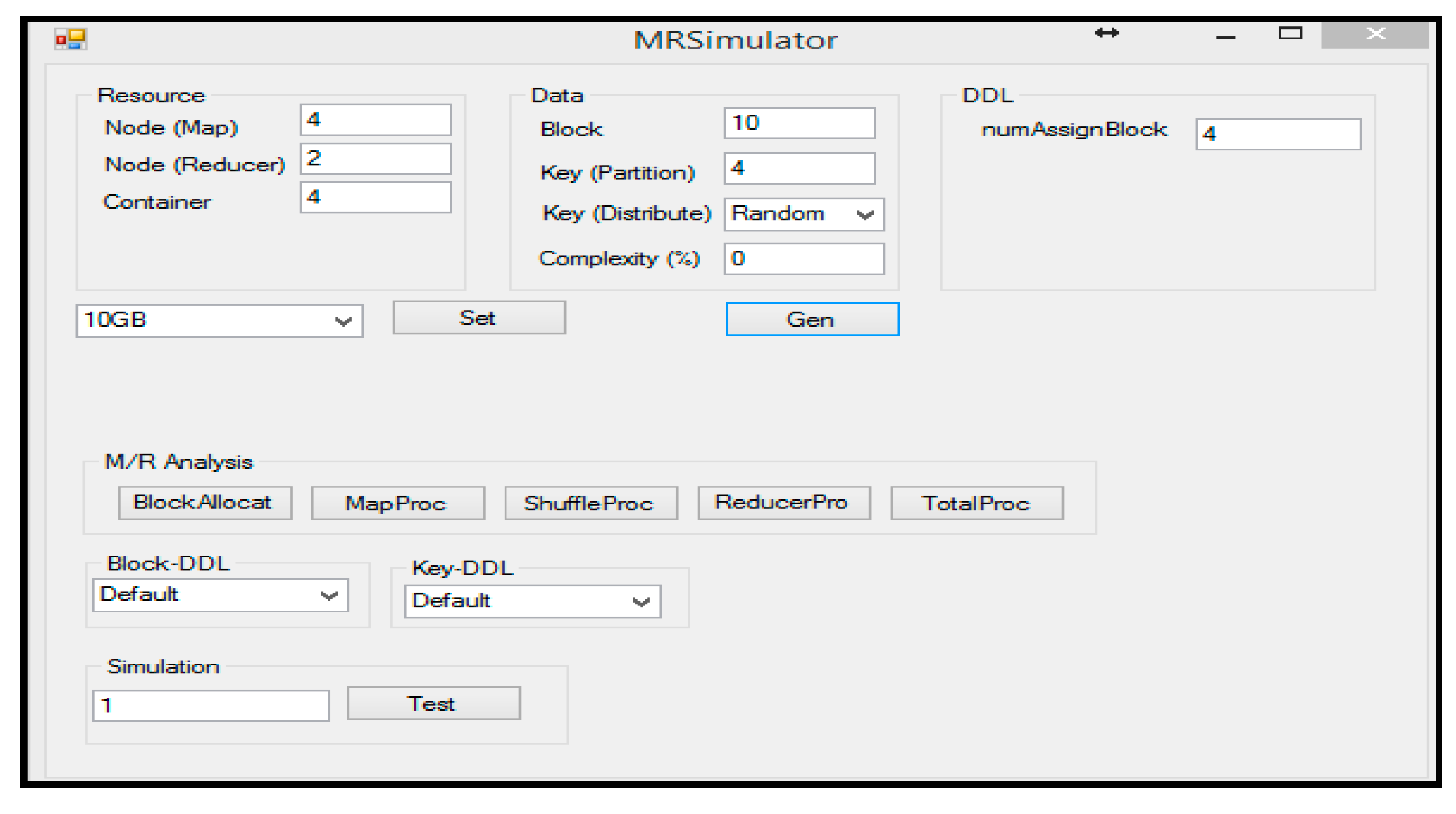
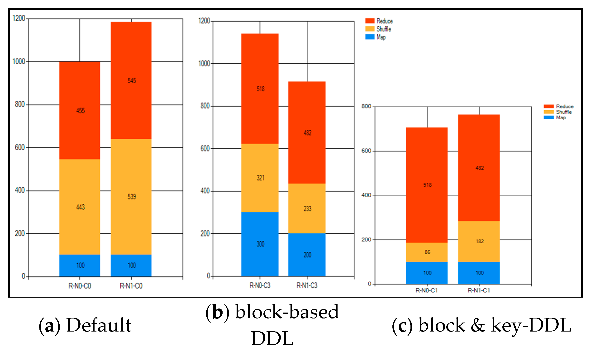
5.2. Hadoop Performance Test on Simulator

The performance of Hadoop depends on many factors, such as the composition of Hadoop cluster, data size, key distribution on blocks, etc. To measure the performance under a variety of conditions, the authors developed a simulator (Figure 16).
The simulator has four control sections: Resource, data, M/R analysis, and data locality methods. Resource is for the hardware setup such as number of slave nodes, number of VMs and size of the input data. The data section is for the characteristic of data such as, number of blocks, number of keys in the block, key distributions and complexity of the block. M/R Analysis is for measuring the performance of the Hadoop system. There are five MR analysis options, i.e., block location, map processing time, shuffle processing time, reduce processing time and total processing time. The simulator can analyze the performance of Hadoop using the five analyses on various environments with the data locality.
Figure 17 shows one sample result of the performance comparison using the simulator. In this case, when block-based DDL and key-based DDL were used together, it outperformed the default MR by 35%. The continued analysis showed a very encouraging result.

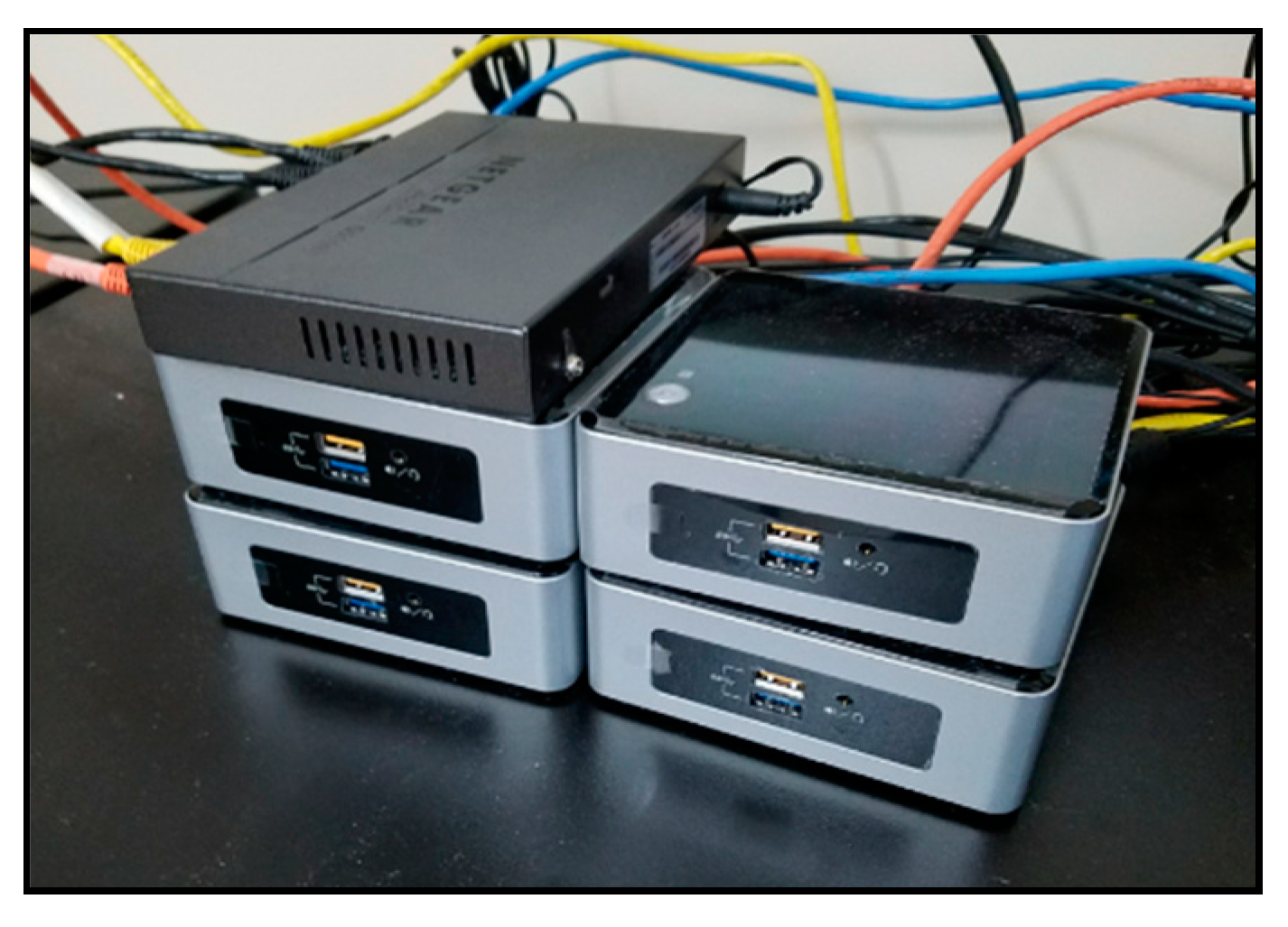
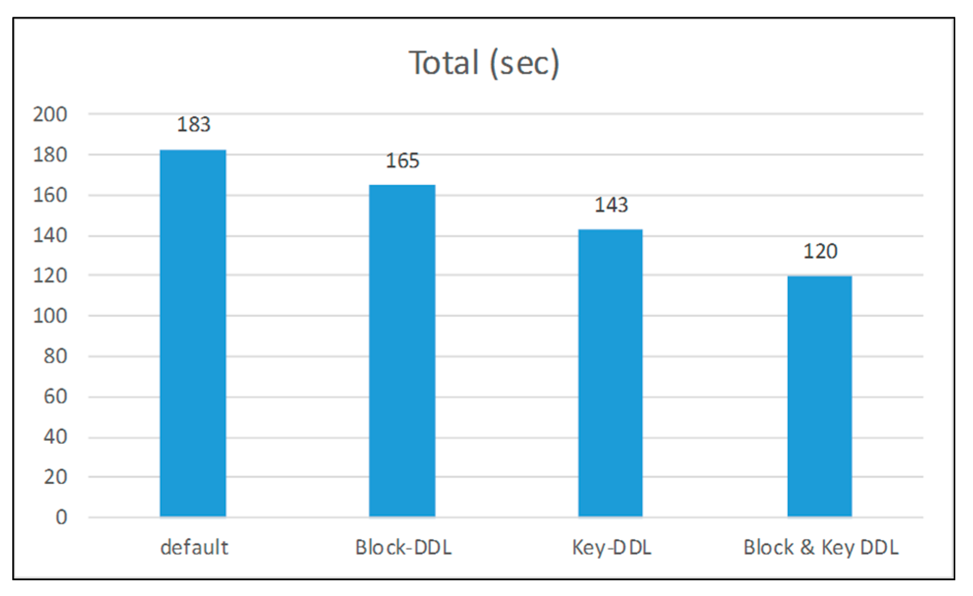
5.3. Hadoop Performance Test on Hardware Implementation

This study tested the data locality performances with hardware implementation to verify the accuracy of the analytical and simulation models. A small Hadoop cluster was configured with five machines, one for the master node and 4 for slave nodes (Figure 18). Each machine was equipped with quad-core Intel Pentium processor, 32 GB eMMC disk (250 MB/s) and 8 GB of 1333 MHz DDR3 memory. A Netgear GS108-Tv2 switch (100 Mbps) was used for the network. Using WordCount benchmark with 1 GB of input data, the authors tested four different methods, i.e., default MR, MR with block-based DDL, MR with key-based DDL, and MR with both block-based and key-based DDL.
The result is shown in Figure 19. The performance improved as more data locality was added. Table 4 shows the same results in ratio in comparison with the default MR. MapReduce with key-based DDL was 21.9% faster than the default MR and 9.8% over the block-based DDL. When block-based and key-based DDL schemes were combined, it was 34.4% faster than default MR. However, the key-based DDL required pre-processing of the data (DDL-aware ETL), so the actual performance improvement was slightly diminished.

6. Conclusions and Future Work

The paper introduced the concept of data locality on HDFS and the Hadoop performance analysis model. The deep data locality on the model was applied to improve the performance of the Hadoop system. The authors made two DDL methods, such as block-based DDL and key-based DDL. The two DDL methods were combined on HDFS and increased over 34.4% more performance than the default MR. The DDL methods on the Hadoop system were tested on a cloud, Hadoop simulation and physical implement Hadoop system. According to the test, the block-based DDL increased the Hadoop performance by 9.8% more than the default MR, and key-based DDL improved it by 21.9% more than the default one. Also, the combined methods increased the Hadoop performance upto 34.4% more than the default method.
For the future work, research into various big data applications in science, engineering, and the business community is required to investigate their data types and applications for the suitability of DDL, and develop algorithms for data transformation as necessary. Also, more research is required about the DDL-aware ETL to apply various applications and data types.

Author Contributions

Formal analysis, S.L.; supervision, Y.K. and J.-Y.J.; writing—original draft, S.L.; writing—review & editing, Y.K. and J.-Y.J.

Funding

This material is based upon the work supported by the National Science Foundation under grant number IIA-1301726.

Conflicts of Interest

The authors declare no conflict of interest. Any opinions, findings, and conclusions or recommendations expressed in this material are those of the author(s) and do not necessarily reflect the views of the National Science Foundation.

References

  1. Gantz, J.; Reisel, D. The Digital Universe in 2020: Big Data, Bigger Digital Shadows, and Biggest Growth in the Far East. Available online: https://www.emc.com/collateral/analyst-reports/idc-digital-universe-united-states.pdf (accessed on 10 June 2019).
  2. Hadoop. Available online: http://hadoop.apache.org/ (accessed on 10 June 2019).
  3. Hadoop YARN. Available online: https://hadoop.apache.org/docs/r2.7.1/hadoop-yarn/hadoop-yarn-site/YARN.html (accessed on 10 June 2019).
  4. Apache Storm. Available online: http://storm.apache.org/ (accessed on 10 June 2019).
  5. Apache Spark. Available online: http://spark.apache.org/ (accessed on 10 June 2019).
  6. Apache HBase. Available online: https://hbase.apache.org/ (accessed on 10 June 2019).
  7. R Open Source Projects. Available online: http://projects.revolutionanalytics.com/rhadoop/ (accessed on 10 June 2019).
  8. MATLAB MapReduce and Hadoop. Available online: http://www.mathworks.com/discovery/matlab-mapreduce-hadoop.html (accessed on 10 June 2019).
  9. Hadoop MapReduce. Available online: https://hadoop.apache.org/docs/r2.7.1/hadoop-mapreduce-client/hadoop-mapreduce-client-core/MapReduceTutorial.html (accessed on 10 June 2019).
  10. Tang, S.; Lee, B.S.; He, B. DynamicMR: A Dynamic Slot Allocation Optimization Framework for MapReduce Clusters. IEEE Trans Cloud Comput. 2014, 2, 333–347. [Google Scholar] [CrossRef]
  11. Membrey, P.; Chan, K.C.C.; Demchenko, Y. A Disk Based Stream Oriented Approach for Storing Big Data. In Proceedings of the 2013 International Conference on Collaboration Technologies and Systems, San Diego, CA, USA, 20–24 May 2013; pp. 56–64. [Google Scholar]
  12. Hou, X.; Ashwin Kumar, T.K.; Thomas, J.P.; Varadharajan, V. Dynamic Workload Balancing for Hadoop MapReduce. In Proceedings of the Fourth IEEE International Conference on Big Data and Cloud Computing, Sydney, Australia, 3–5 December 2014; pp. 56–62. [Google Scholar]
  13. Hammoud, M.; Sakr, M.F. Locality-Aware Reduce Task Scheduling for MapReduce. In Proceedings of the Third IEEE International Conference on Cloud Computing Technology and Science, Athens, Greece, 29 November–1 December 2011; pp. 570–576. [Google Scholar]
  14. Dai, X.; Bensaou, B. A Novel. Decentralized Asynchronous Scheduler for Hadoop. Communications QoS, Reliability and Modelling Symp. In Proceedings of the 2013 IEEE Global Communications Conference, Atlanta, GA, USA, 9–13 December 2013; pp. 1470–1475. [Google Scholar]
  15. Zhu, H.; Chen, H. Adaptive Failure Detection via Heartbeat under Hadoop. In Proceedings of the IEEE Asia -Pacific Services Computing Conference, Jeju, Korea, 12–15 December 2011; pp. 231–238. [Google Scholar]
  16. Nishanth, S.; Radhikaa, B.; Ragavendar, T.J.; Babu, C.; Prabavathy, B. CoRadoop++: A Load Balanced Data Colocation in Radoop Distributed File System. In Proceedings of the IEEE 5th International Conference on Advanced Computing, ICoAC 2013, Chennai, India, 18–20 December 2013; pp. 100–105. [Google Scholar]
  17. Elshater, Y.; Martin, P.; Rope, D.; McRoberts, M.; Statchuk, C. A Study of Data Locality in YARN. In Proceedings of the IEEE International Congress on Big Data, Santa Clara, CA, USA, 29 October–1 November 2015; pp. 174–181. [Google Scholar]
  18. Qin, P.; Dai, B.; Huang, B.; Xu, G. Bandwidth-Aware Scheduling with SDN in Hadoop: A New Trend for Big Data. IEEE Syst. J. 2015, 11, 1–8. [Google Scholar] [CrossRef]
  19. Lu, X.; Islam , N.S.; Wasi-ur-Rahman, M.; Jose, J.; Subramoni, H.; Wang, H.; Panda, D.K. High-Performance Design of Hadoop RPC with RDMA over InfiniBand. In Proceedings of the 42nd IEEE International Conference on Parallel Processing, Lyon, France, 1–4 October 2013; pp. 641–650. [Google Scholar]
  20. Basak, A.; Brnster, I.; Ma, X.; Mengshoel, O.J. Accelerating Bayesian network parameter learning using Hadoop and MapReduce. In Proceedings of the 1st International Workshop on Big Data, Streams and Heterogeneous Source Mining: Algorithms, Systems, Programming Models and Applications, Beijing, China, 12 August 2012; pp. 101–108. [Google Scholar]
  21. Iwazume, M.; Iwase, T.; Tanaka, K.; Fujii, H.; Hijiya, M.; Haraguchi, H. Big Data in Memory: Benchimarking In Memory Database Using the Distributed Key-Value Store for Machine to Machine Communication. In Proceedings of the 15th IEEE/ACIS International Conference on Software Engineering, Artificial Intelligence, Networking and Parallel/Distributed Computing, Beijing, China, 30 June–2 July 2014; pp. 1–7. [Google Scholar]
  22. SAP HANA. Available online: http://hana.sap.com/abouthana.html (accessed on 10 June 2019).
  23. Islam, N.S.; Wasi-ur-Rahman, M.; Lu, X.; Shankar, D.; Panda, D.K. Performance Characterization and Acceleration of In-Memory File Systems for Hadoop and Spark Applications on HPC Clusters. In Proceedings of the International Conference on Big Data, IEEE Big Data, Santa Clara, CA, USA, 29 October–1 November 2015; pp. 243–252. [Google Scholar]
  24. Hadoop HDFS. Available online: https://issues.apache.org/jira/browse/HDFS/ (accessed on 10 June 2019).
  25. Lee, S. Deep Data Locality on Apache Hadoop. Ph.D. Thesis, The University of Nevada, Las Vegas, NV, USA, 10 May 2018. [Google Scholar]
  26. MapR. Available online: https://www.mapr.com/products/product-overview/shark (accessed on 10 June 2019).
  27. Lee, S.; Jo, J.-Y.; Kim, Y. Survey of Data Locality in Apache Hadoop. In Proceedings of the 4th IEEE/ACIS International Conference on Big Data, Cloud Computing, and Data Science Engineering (BCD), Honolulu, HI, USA, 29–31 May 2019. [Google Scholar]
  28. Lee, S.; Jo, J.-Y.; Kim, Y. Key based Deep Data Locality on Hadoop. In Proceedings of the IEEE International Conference on Big Data, Seattle, WA, USA, 10–13 December 2018; pp. 3889–3898. [Google Scholar]
  29. Lee, S.; Jo, J.-Y.; Kim, Y. Performance Improvement of MapReduce Process by Promoting Deep Data Locality. In Proceedings of the 3rd IEEE International Conference on Data Science and Advanced Analytics (DSAA), Montreal, QC, Canada, 17–19 October 2016; pp. 292–301. [Google Scholar]
  30. IBM, InfoSphere Data Stage. Available online: https://www.ibm.com/ms-en/marketplace/datastage (accessed on 10 June 2019).
  31. Oracle. Data Integrator. Available online: http://www.oracle.com/technetwork/middleware/data-integrator/overview/index.html (accessed on 10 June 2019).
  32. Informatica. PowerCenter. Available online: https://www.informatica.com/products/data-integration/powercenter.html#fbid=uzsZzvdWlvX (accessed on 10 June 2019).
  33. DataStream. TeraStream. Available online: http://datastreamsglobal.com/ (accessed on 10 June 2019).
  34. Cloudlab. Available online: https://www.cloudlab.us/ (accessed on 10 June 2019).
Figure 1. MapReduce stages.
Information 10 00222 g001
Figure 2. Hadoop locality research areas.
Information 10 00222 g002
Figure 3. Locality type.
Information 10 00222 g003
Figure 4. Data locality schemes.
Information 10 00222 g004
Figure 5. Time variables for each stage.
Information 10 00222 g005
Figure 6. Map function time.
Information 10 00222 g006
Figure 7. Processing time of the first stage on the mapper (i).
Information 10 00222 g007
Figure 8. First stage calculation graph.
Information 10 00222 g008
Figure 9. Model of the second stage.
Information 10 00222 g009
Figure 10. Data locality in the second stage.
Information 10 00222 g010
Figure 11. Second stage calculation graph (T2).
Information 10 00222 g011
Figure 12. Total Hadoop processing time calculation graph.
Information 10 00222 g012
Figure 13. Block locations.
Information 10 00222 g013
Figure 14. Shuffle stage comparison.
Information 10 00222 g014
Figure 15. Big-ETL versus DDL-aware Big-ETL.
Information 10 00222 g015
Figure 16. Simulator GUI.
Information 10 00222 g016
Figure 17. Performance comparisons on the simulator.
Information 10 00222 g017
Figure 18. Hadoop testbed.
Information 10 00222 g018
Figure 19. Performance comparison of total time.
Information 10 00222 g019
Table 1. Constants and time symbol.
Constant SymbolDefinitionTime SymbolDefinition
αProcessing time for one blockT1Processing time of First Stage (TM + TS)
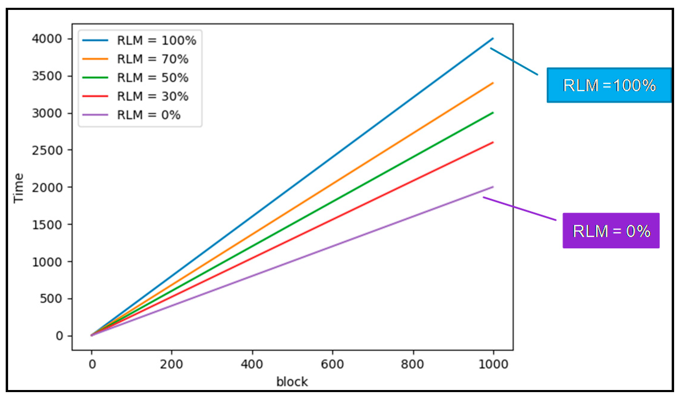
β Transferring time of one block under Rack-LocalTMProcessing time of Map function
TSProcessing time of Sort, Spill, Fetch in Shuffle
δTransferring time of one block under Off-RackT2Processing time of Second Stage (TT + TR)
TTProcessing time of Transfer in Shuffle
γProcessing time of Sort, Spill and Fetch for one blockTRProcessing time of Reduce function
TTotal processing time of Hadoop
Table 2. Other variables.
SymbolDefinitionSymbolDefinition
MNumber of Mapper in MapBiSet of allocated blocks in Mapper (i), {b1, b2, …, bB}
RNumber of Reducer in Reduce|Bi|Total number of allocated blocks in Mapper (i)
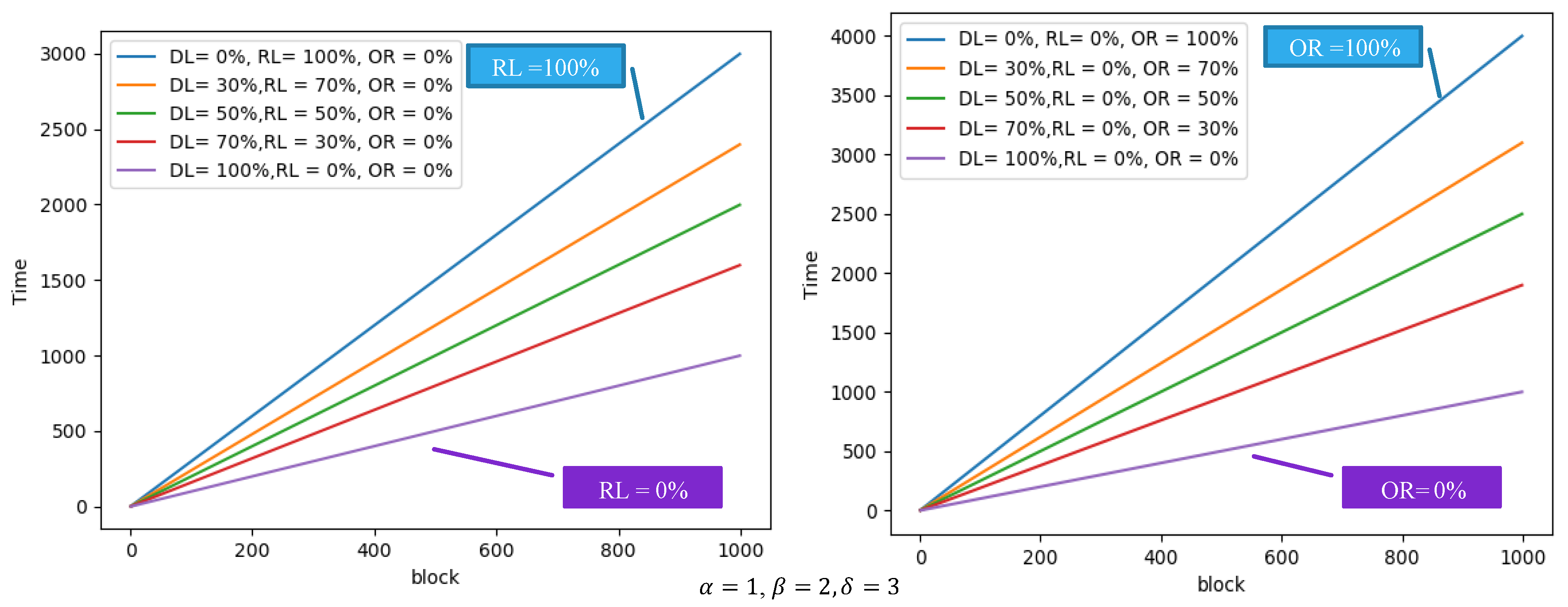
RLMiNumber of Rack Local Map (RLM) in Mapper (i)PrRatio of Partition in Mapper, {P1, P2, …, Pr}
iMapper IDRDLRatio of Disk-Local
jReducer IDRRLRatio of Rack-Local
bBlock IDRORRatio of Off-Rack
Table 3. Terasort with Hadoop Default (DBPP) and block-based DDL (LNBPP).
Map (s)Shuffle (s)Total (min) Map (s)Shuffle (s)Total (min) Map (s)Shuffle (s)Total (min)
Default-Job1-30G2646327Default-Job1-60G2592971Default-Job1-120G282345165
Default-Job2-30G3043127Default-Job2-60G2790676Default-Job2-120G321968165
LNBPP-Job1-30G2229221LNBPP-Job1-60G2472159LNBPP-Job1-120G241475150
LNBPP-Job2-30G2032825LNBPP-Job2-60G2277162LNBPP-Job2-120G251647150
Decrease Time (%)25%30.7%14.8%Decrease Time (%)11.5%18.7%17.7%Decrease Time (%)18.3%27.6%9%
* Default-Job1-30G: “Job1 executing the Default policy with 30 GB data”. ** LNBPP-Job1-30G: “Job1 executing LNBPP with 30 GB data”.
Table 4. Improvement of Hadoop performance by DDL.
Block-DDLKey-DDLBlock& Key-DDL
Default9.8%21.9%34.4%
Block-DDLN/A13.3%27.3%
Key-DDLN/AN/A16.1%

