An Underground Radio Wave Propagation Prediction Model for Digital Agriculture


Department of Computer and Information Technology, Purdue University, West Lafayette, IN 47907, USA
Information 2019, 10(4), 147; https://doi.org/10.3390/info10040147
Submission received: 20 March 2019
/
Revised: 10 April 2019
/
Accepted: 16 April 2019
/
Published: 18 April 2019
(This article belongs to the Section Information and Communications Technology)
Abstract
:Underground sensing and propagation of Signals in the Soil (SitS) medium is an electromagnetic issue. The path loss prediction with higher accuracy is an open research subject in digital agriculture monitoring applications for sensing and communications. The statistical data are predominantly derived from site-specific empirical measurements, which is considered an impediment to universal application. Nevertheless, in the existing literature, statistical approaches have been applied to the SitS channel modeling, where impulse response analysis and the Friis open space transmission formula are employed as the channel modeling tool in different soil types under varying soil moisture conditions at diverse communication distances and burial depths. In this article, an electromagnetic field analysis is presented as an enhanced monitoring approach for subsurface radio wave propagation and underground sensing applications in the field of digital agriculture. The signal strength results are shown for different distances and depths in the subsurface medium. The analysis shows that the lateral wave is the dominant wave in subsurface communications. Moreover, the shallow depths are more suitable for soil moisture sensing and long-range underground communications. The developed paradigm leads to advanced system design for real-time soil monitoring applications.
1. Introduction
The subsurface radio wave propagation is vital for sending and receiving wireless signals in the next-generation precision agriculture Internet of Underground Things (IOUT) [1,2,3]. The Signals in the Soil (SitS) wireless communication approach has only focused mainly on the empirical methods [3,4,5,6,7,8,9,10,11,12,13,14,15,16], thereby ignoring the importance of the physical characteristics behind the fundamental electromagnetic subsurface physics [17,18,19,20,21,22].
The subsurface wireless underground communications involve two different material half-spaces (e.g., soil and air half-space). Moreover, both the transmitter and receiver can be placed in any of the half-spaces, which leads to three different types of subsurface wireless channels, which are different from Over-The-Air (OTA) wireless communications channels. These unique channels involve the soil-to-air half-space, air-to-soil half-space, and subsurface on-soil communications. Hence, the consideration of electromagnetic fields becomes very important in subsurface wireless communications. Therefore, the aim of this article is to present subsurface electromagnetic field analysis (an analytical solution) involving soil and air half-spaces, which is based on Maxwell’s physics. This article presents a subsurface radio wave propagation prediction model based on the fundamental EM analysis related to subsurface propagation modeling that considers the electromagnetic field of a unit vertical and horizontal electric dipole in the presence of a plane boundary.
This underground signals analysis is useful for subsurface radio wave propagation and underground antenna characterization in soil medium. It is also applicable to radio wave propagation in forests and other environments where there is a need for accurate wireless channel models that can be used to produce actual empirical results without the need for any linear and nonlinear regression. In addition, these channel models will also aid in the widespread deployment of agricultural wireless sensor networks, the development of improved efficiency protocols, and the improved subsurface communication system design. In this article, a direct approach based on electromagnetic field analysis has been applied to radio wave propagation in the stratified soil medium for smart farming applications in precision agriculture and the Internet of Underground Things.
The rest of the article is organized as follows: the background and related work is presented in Section 2. The electromagnetic field of a unit vertical electric dipole in the presence of a plane boundary is analyzed in Section 3. In Section 4, the electromagnetic field of a horizontal electric dipole in the presence of a plane boundary is discussed. Model evaluations and results are presented in Section 5. The applications of this work are discussed in Section 6. The paper concludes in Section 7.
2. Background and Related Work
The Per- and Poly-Fluoroalkyl Substances’ (PFAS) management techniques are important in order to establish a proper detection and analysis methods to achieve greater efficiency [23]. Timely PFAS management minimizes risks to humans and environment. PFAS treatment approaches that result from improper detection lead to detrimental environmental effects. Proper PFAS detection will help to reduce the potential of chemical leaching to the soil and water resources and also into the environment.
Among existing techniques, Granular Activated Carbon (GAC) is a growing technology in PFAS treatment in water [23,24,25]. However, there is a significant lack of data and procedure development in terms of fundamental understanding and quantification of the medium properties. The adsorptive and destructive technologies are considered for both soils and water [26,27,28]. Other remediation approaches are anion-exchange, ozofractionation, chemical oxidation, electrochemical oxidation, sonolysis, soil stabilization, and thermal technologies [29,30,31,32,33].
These treatment technologies are not best suited to provide PFAS management systems with almost real-time sensing data to facilitate fast decision making [34,35,36]. Thus, proper treatment cannot be applied at the right place of the waste system at the right time. Failure to consider the spatial variability of PFAS in management decisions results in inefficient management. Accordingly, the potential of chemical leaching from the landfill surface is increased. Timely information of temporal and spatial soil PFAS patterns can significantly aid PFAS decision makers in better managing their treatment operations to achieve higher treatment efficiency. The real-time knowledge of spatial PFAS demand can also further advance our understanding of variable physico-chemical and biological dynamics. Accordingly, more effective management and treatment strategies can be developed for PFAS removal.
The first generation of wireless underground communication systems was developed in the 2000s and was based on the application of the Over-The-Air (OTA) Friis transmission formula to the underground wireless channel [6,15]. In the early 2010s, the second generation of wireless underground communications was developed based on the impulse response analysis and advanced multi-carrier techniques [10,37]. The major development in the second-generation wireless underground communications is the statistical model of the underground channel, which has been developed based on the extensive empirical campaign both in field and testbed environments [9,10]. The model can predict the Root Mean Square (RMS) delay spread, coherence bandwidth, and path loss. Because the statistical model has been developed based on the statistical and information theoretic perspective, it lacks the insight into the physics of subsurface radio wave propagation, which can only be provided by Maxwell–Poynting theory-based signal processing. However, there is no underground channel model available based on the subsurface electromagnetic-based signal processing analysis, and only the numerical evaluations and results have been presented. Accordingly, to gain the physical insight into the propagation of wireless underground communication waves and to ensure that the wireless underground communication system performance is optimal in different subsurface media, it is vital to have an underground propagation prediction model based on electromagnetic using physics principals applicable to radiation efficiency, antenna design, and power transfer at different distances and depths in the soil medium.
Recently, many advanced analytical solutions have been reported in the literature for the Sommerfeld integral [38,39,40,41,42,43]. An alternative solution to the Sommerfeld integral based on the branch-cut integral has been discussed in [42]. An analysis of a two-layered structure using the longitudinal spectrum for space waves, surface waves, and Zenneck waves has been presented in [43]. A Zenneck wave-based UGchannel model has been developed in [44]. However, this model was developed using the approximation of the EM analysis and has higher error.
The aim of this paper is to present the wireless underground communications prediction model for different distances, and depths, under different soil moisture levels, capable of predicting in different soil textures. This work is the first work to develop a subsurface radio wave propagation prediction model completely based on the electromagnetic-based signal processing analysis.
3. The Electromagnetic Field of a Unit Vertical Electric Dipole in the Presence of a Plane Boundary
The change of the soil moisture impacts the signal propagation in the underground soil medium. The increase in Volumetric Water Content (VWC) leads to a decrease in the received signal strength at the underground receiver. In this section, we develop the field solutions by ascertaining the VWC percentage by using underground sensors and accordingly using Peplinski’s model to obtain the complex permittivity of the soil under consideration. The obtained complex permittivity value for a given VWC level is employed in the model along with other soil parameters (e.g., soil type, soil bulk density, burial depth in medium, and communication distance) to predict radio wave propagation for a particular agricultural field. Accordingly, the subsurface communication system can be tailored for site-specific and soil-specific applications. Overall, the developed model can be effectively used to predict propagation characteristics in the soil medium with the change in soil moisture for digital agriculture applications. These developments are vital to understanding the properties of subsurface waves and provide useful insights for system design.
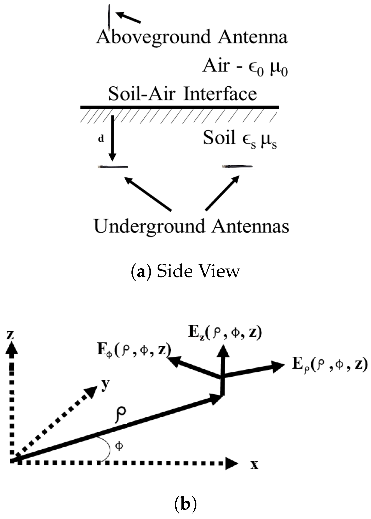
A list of notations used in the paper is given in the “Abbreviations”. The electromagnetic field generated by a vertical electric dipole near the boundary [18] between two quite different material half-spaces is obtained from the explicit integrals for the component differentiation of the electromagnetic field. The vertical dipole with the unit electric moment (i.e., ) is located on the downward-directed z-axis at a distance d from the origin of the coordinates on the interface, i.e., the -plane. A drawing of the geometry of the underground antenna is shown in Figure 1. The electromagnetic field is to be determined at an arbitrary point in rectangular or in cylindrical coordinates. The lower half-space () is Region 1, and the upper half-space () is Region 2. The two regions are characterized by the complex wave numbers , where and with . It is assumed that both regions are nonmagnetic, so that . The time dependence is used.
From Maxwell’s equations, we obtain an ordinary differential equation for :
with:
Other components can be expressed by ,
The equations have been solved in [45], and the complete results for the two regions are summarized below. The following shorthand notation is used:
Region 1, :
Region 2, :
The electromagnetic field at an arbitrary position is the integrals of the components:
In order to evaluate the integrals for the components of the electromagnetic field at in Region 1 when the vertical electric dipole is also in Region 1 at , it is convenient to examine separately for different parts. These are the direct field, the reflected field due to an ideal image, the lateral-wave field, and a correction for the reflected field when this is not accurately that of an ideal image (Figure 2). Specifically, let:
The direct field is given by:
The ideal reflected field is the field at due to an image antenna at . The electric moment of the image is the negative of that of the source.
Given conditions:
the rest field can be written in the following compact form:
where the radial functions and are defined as follows:
Here:
is called the numerical distance. The function is:
where is the Fresnel integral. When the argument p is sufficiently great, specifically when:
and can be approximated as:
If the conditions in (30) are not satisfied, the complete electromagnetic field in Region 1 is given by:
For the complete field in Region 2, the following results are obtained.
where:
The approximations are valid when the conditions:
are satisfied. In this case, and in amplitude, , and the terms of the order are neglected.
4. The Electromagnetic Field of a Horizontal Electric Dipole in the Presence of a Plane Boundary
Consider the x-directed horizontal electric dipole [18] at the point on the downward-directed z-axis in the half-space (Region 1) defined by . Region 2 is defined by . The wave numbers of the two regions are , where and . It is assumed that both regions are nonmagnetic, so that . Based on Maxwell’s equations, the following results are reached:
Moreover, the following ordinary differential equations for and are also obtained:
where:
The six components of the electromagnetic field in the cylindrical coordinates are:
Region 1, :
Where two signs appear, the upper one is for , and the lower is for (see Figure 3).
Region 2, :
In these equations,
and is the integral form of the Bessel function. It is:
With conditions:
the expressions in Region 1 can be simplified.
.
In these formulas,
where:
and:
is the Fresnel integral.
In the simplified expressions, the direct field is given by all terms multiplied by ; the complete reflected field includes all terms with the factor ; and the lateral-wave field consists of the terms multiplied by . The quantities and represent spherical waves traveling radially outward from the dipole at or the image dipole at . The quantity suggests a plane wave that travels upward in Region 1 from the source at to the boundary at , then radially outward in Region 2 as a cylindrical wave to , and finally, vertically downward from the boundary in Region 1 as a plane wave to the point of observation at .
5. Model Evaluations and Results
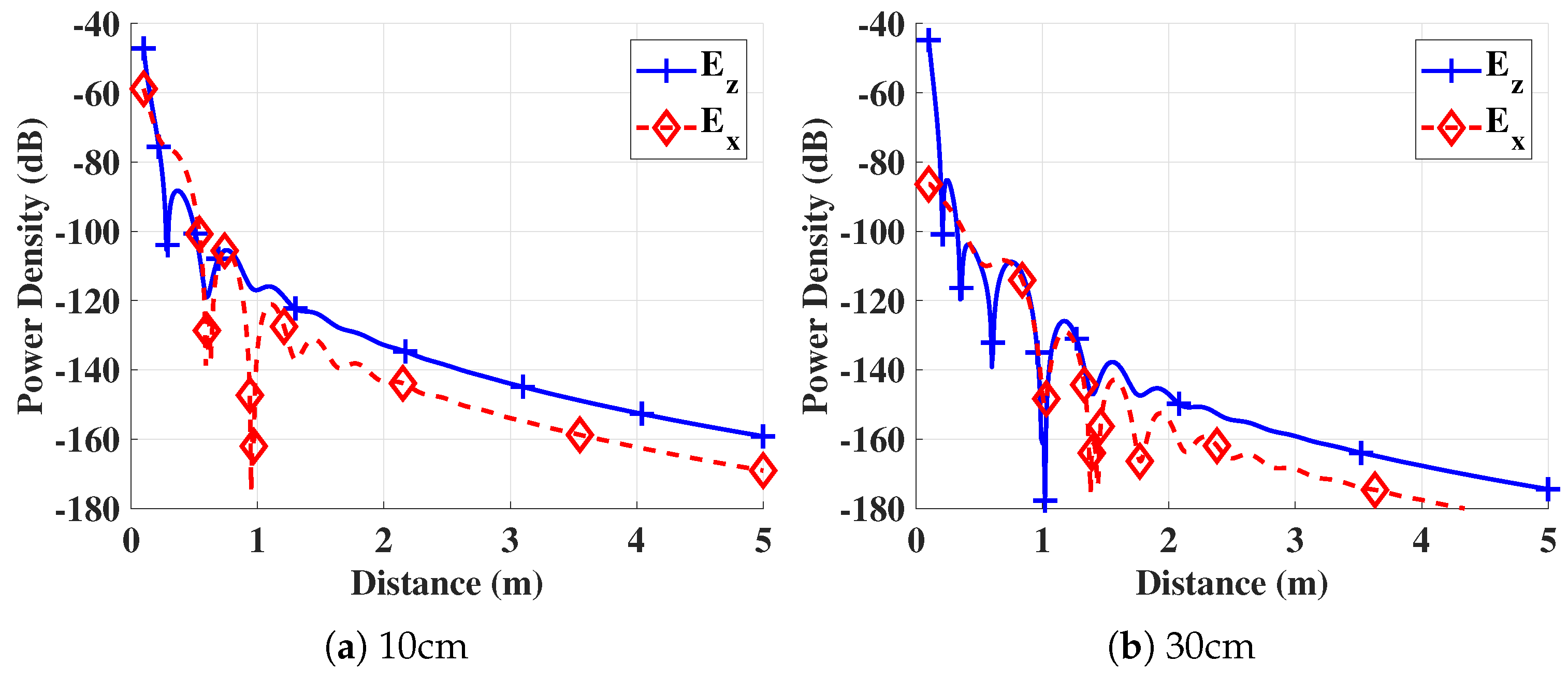
In order to show the path loss in subsurface wireless underground communications, model evaluations were done, and results are shown for a horizontal electric dipole in the presence of a plane boundary. The Volumetric Water Content (VWC) was 20% (obtained through the complex permittivity [46,47]). Due to the lossy characteristics of the soil medium, it is represented through complex permittivity. Moreover, because the soil propagation medium is non-magnetic, the permeability of the free space () was used (Section 3). A total of five transmitter burial depths depths of 10 cm, 20 cm, 30 cm, 40 cm, and 50 cm were considered for the evaluation of an x-directed horizontal electric dipole. The lateral wave power density magnitude is shown as a function of distance. The communication distances up to 5 m were evaluated at the frequency of 433 MHz. From all six components of the lateral signal (e.g., three electric and three magnetic components), the results are only shown for the components and ( with ) in the subsurface region.
The comparison of the power density of and components at different burial depths is shown in Figure 4. It can be observed that at a 10-cm depth (Figure 4a), the power density of the horizontal component , which is the lateral wave component (,0,z), was on par with the component. However, for distances greater than 1 m, the horizontal component became 11 dB weaker as compared to the . This happened because of the higher attenuation of the component in the medium. This became clearer when the depth increased to 30 cm (Figure 4b). At a 30-cm depth, the lateral component had a strong power density at shorter distances (<1 m). With the increase in distance, the horizontal component decreased gradually. Similar results have also been obtained in [10], and those empirical results showing the dominance of the lateral wave confirm the accuracy of this underground propagation prediction model. Moreover, the model accurately captured the physical propagation differences due to the propagation of different components.
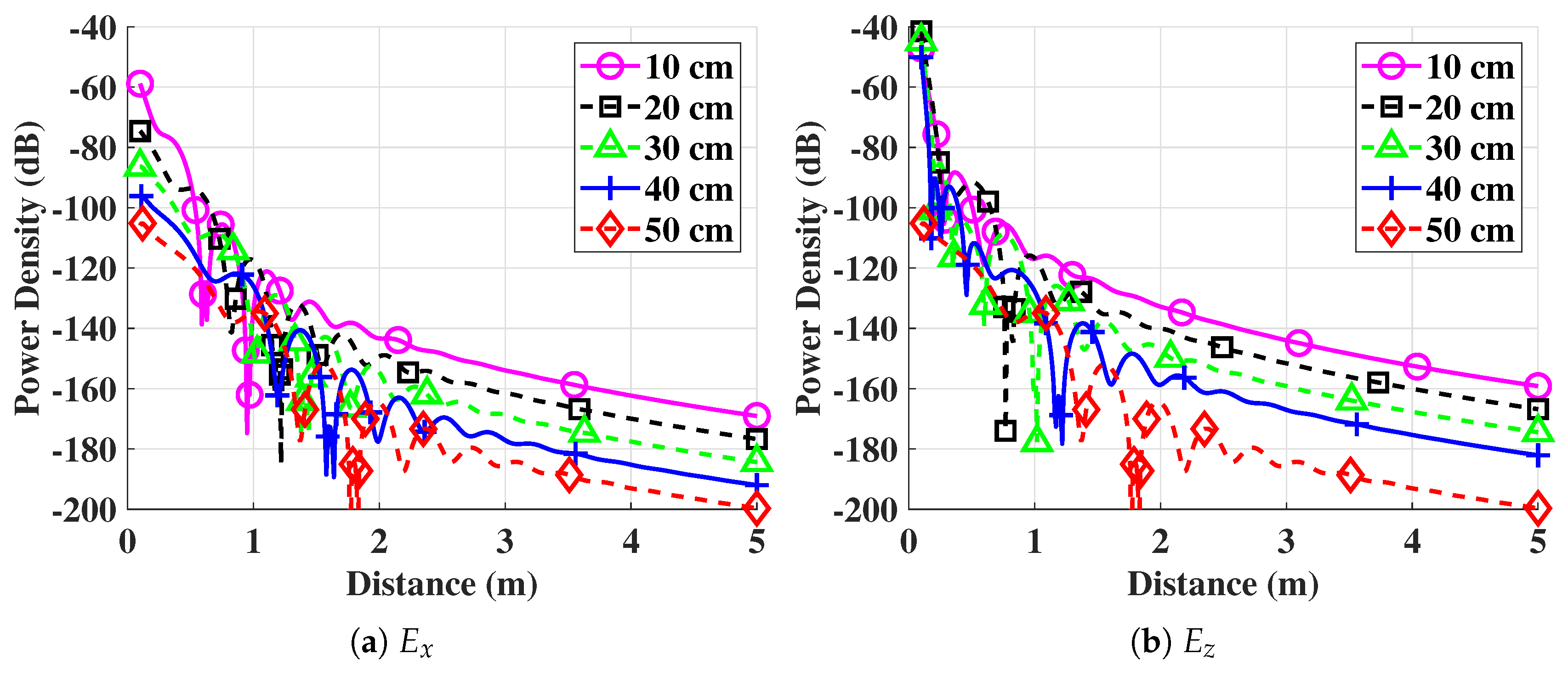
The results of the numerical evaluations of the signal strength for different depths for both the and components are shown in Figure 5. The abrupt drops in the signal strength can be observed for a distance value of less than 2 m for both components. This happened because when the wave traveled in the soil medium, then a cross-sectional plane was formed at a wavelength. At this cross-sectional plane, the intensity of the signal was at the positive maximum value. However, half-way, the reversed direction of the electric field vector was at the negative maximum value, which led to these drops in the power density. At the higher distances, this effect became less significant because of the low signal strength caused by the higher attenuation of the wave traveling in the subsurface medium. Moreover, it can also be observed that the signal strength of the dominant lateral wave decreased with the increase in the depth and distance. The developed model can also capture the water sensitivity of the soil medium.
6. Applications
For an underground communications’ system design, the propagation characteristics of the subsurface soil environment should be determined accurately. This knowledge is also important for underground network design in the Internet of Underground Things (IOUT) in precision agriculture. For accurate soil moisture sensing, the location of the placement of underground nodes plays an important role in node deployment. The analysis presented in the paper can be used to determine the path loss between the underground Transmitter-Receiver pair (T-R), which helps to achieve the maximum coverage area in the crop field with optimal deployment. This model also provides information about the ideal depths in the underground medium. The model output also aids in selecting optimal communication parameters (e.g., modulation scheme and transmit power) for the wireless channel in a particular environment. Without the use of the model, this path loss information can only be obtained through empirical evaluations in the field. These field measurements are site specific, harder to implement in complex field environments, and lead to inefficient and delayed system deployment.
7. Conclusions
In this article, a physical electromagnetic analysis related to subsurface propagation modeling, which considers the electromagnetic field of a unit vertical and horizontal electric dipole in the presence of a plane boundary, has been carried out. It has been shown that the lateral wave is the dominant wave in subsurface communications, and shallow depths are more suitable for long-range communications and sensing. This analysis forms the basis of subsurface radio wave propagation modeling in the stratified soil medium for smart farming applications in precision agriculture [13,20,48,49,50,51] and urban underground infrastructure monitoring [52,53].
Furthermore, we highlight that the empirical evaluations of UG solutions under realistic application requirements is essential due to the interplay between the physical soil medium and radios. The main contribution of this paper is to present the physics-based subsurface propagation prediction model. To this end, we have evaluated the results and have shown the agreement with the empirical channel measurement results obtained through extensive impulse response measurements in an indoor and field testbed. The change of the soil moisture impacts the signal propagation in the underground soil medium [37]. The increase in VWC leads to a decrease in the received signal strength at the underground receiver [10]. The developed approach works by ascertaining the VWC percentage by using underground sensors and accordingly using Peplinski’s model [46] to obtain the complex permittivity of the soil under consideration. The obtained complex permittivity value for a given VWC level can accordingly be inserted into the model along with other soil parameters (e.g., soil type, soil bulk density, burial depth in medium, and communication distance) to predict radio wave propagation for a particular agricultural field. Accordingly, the subsurface communication system can be tailored for site-specific and soil-specific applications. Overall, the developed model can be effectively used to predict propagation characteristics in the soil medium with a change in soil moisture for digital agriculture applications. For future work, we will perform the evaluation of the developed solutions through both unit-level experimentation and simulations and application-level evaluations. The wide variety of applications of UG communications including agriculture, soil contaminants detection, mining, transportation, and border patrol results in a diverse set of requirements that can benefit from this approach.
Funding
This research received no external funding.
Acknowledgments
Publication of this article was funded in part by the Purdue University Libraries Open Access Publishing Fund.
Conflicts of Interest
The authors declare no conflict of interest.
Abbreviations
The following abbreviations are used in this manuscript:
| Notation | Description |
| wavenumber in the soil | |
| wavenumber in the air | |
| wavelength in the soil | |
| phase constant | |
| attenuation constant | |
| permittivity of soil | |
| permeability of free space | |
| l | half length of antenna |
| angular frequency | |
| antenna impedance | |
| transmission line impedance | |
| reflected electric field | |
| reflected current | |
| current amplitude | |
| reflected impedance | |
| characteristics impedance | |
| radiation resistance | |
| current distribution along the antenna | |
| soil-air interface adjusted impedance | |
| return loss | |
| resonant frequency | |
| over-the-air frequency | |
| bandwidth | |
| h | burial depth |
| refractive index of air | |
| refractive index of soil | |
| volumetric water content | |
| bulk density | |
| particle density | |
| , , and | empirical constant |
| , | real and imaginary part of the permittivity of soil |
| S and C | sand and clay particle percentage |
| and | relative permittivity of free water, real and imaginary |
| effective conductivity of soil | |
| , | limit of permittivity of water |
| static permittivity of water | |
| relaxation time of water |
References
- Vuran, M.C.; Salam, A.; Wong, R.; Irmak, S. Internet of Underground Things in Precision Agriculture: Architecture and Technology Aspects. Ad Hoc Netw. 2018, 81, 160–173. [Google Scholar] [CrossRef]
- Vuran, M.C.; Salam, A.; Wong, R.; Irmak, S. Internet of Underground Things: Sensing and Communications on the Field for Precision Agriculture. In Proceeding of the 2018 IEEE 4th World Forum on Internet of Things (WF-IoT) (WF-IoT 2018), Singapore, 5–8 February 2018. [Google Scholar]
- Salam, A.; Vuran, M.C.; Irmak, S. Di-Sense: In situ real-time permittivity estimation and soil moisture sensing using wireless underground communications. Comput. Netw. 2019, 151, 31–41. [Google Scholar] [CrossRef]
- Akkaş, M.A. Channel Modeling of Wireless Sensor Networks in Oil. Wirel. Pers. Commun. 2017, 95, 4337–4355. [Google Scholar] [CrossRef]
- Akyildiz, I.F.; Stuntebeck, E.P. Wireless Underground Sensor Networks: Research Challenges. Ad Hoc Netw. J. 2006, 4, 669–686. [Google Scholar] [CrossRef]
- Akyildiz, I.F.; Sun, Z.; Vuran, M.C. Signal Propagation Techniques for Wireless Underground Communication Networks. Phys. Commun. J. 2009, 2, 167–183. [Google Scholar] [CrossRef]
- Jabbar, S.; Asif Habib, M.; Minhas, A.A.; Ahmad, M.; Ashraf, R.; Khalid, S.; Han, K. Analysis of Factors Affecting Energy Aware Routing in Wireless Sensor Network. Wirel. Commun. Mob. Comput. 2018, 2018, 9087269. [Google Scholar] [CrossRef]
- Konda, A.; Rau, A.; Stoller, M.A.; Taylor, J.M.; Salam, A.; Pribil, G.A.; Argyropoulos, C.; Morin, S.A. Soft Microreactors for the Deposition of Conductive Metallic Traces on Planar, Embossed, and Curved Surfaces. Adv. Funct. Mater. 2018, 28, 1803020. [Google Scholar] [CrossRef]
- Salam, A.; Vuran, M.C.; Irmak, S. Towards Internet of Underground Things in Smart Lighting: A Statistical Model of Wireless Underground Channel. In Proceedings of the 14th IEEE International Conference on Networking, Sensing and Control (IEEE ICNSC), Calabria, Italy, 16–18 May 2017. [Google Scholar]
- Salam, A.; Vuran, M.C.; Irmak, S. Pulses in the Sand: Impulse Response Analysis of Wireless Underground Channel. In Proceedings of the 35th Annual IEEE International Conference on Computer Communications (IEEE INFOCOM 2016), San Francisco, CA, USA, 10–14 April 2016. [Google Scholar]
- Salam, A.; Vuran, M.C. Wireless Underground Channel Diversity Reception with Multiple Antennas for Internet of Underground Things. In Proceedings of the 2017 IEEE International Conference on Communications (ICC), Paris, France, 21–25 May 2017. [Google Scholar]
- Salam, A.; Vuran, M.C. Smart Underground Antenna Arrays: A Soil Moisture Adaptive Beamforming Approach. In Proceedings of the IEEE Conference on Computer Communications (INFOCOM 2017), Atlanta, GA, USA, 1–4 May 2017. [Google Scholar]
- Salam, A. Pulses in the Sand: Long Range and High Data Rate Communication Techniques for Next Generation Wireless Underground Networks; ETD Collection for University of Nebraska: Lincoln, NE, USA, 2018. [Google Scholar]
- Saeed, N.; Al-Naffouri, T.Y.; Alouini, M.S. Towards the Internet of Underground Things: A Systematic Survey. arXiv 2019, arXiv:1902.03844. [Google Scholar]
- Vuran, M.C.; Akyildiz, I.F. Channel model and analysis for wireless underground sensor networks in soil medium. Phys. Commun. 2010, 3, 245–254. [Google Scholar] [CrossRef]
- Sun, Z.; Akyildiz, I. Magnetic Induction Communications for Wireless Underground Sensor Networks. IEEE Trans. Antennas Propag. 2010, 58, 2426–2435. [Google Scholar] [CrossRef]
- Wait, J.; Fuller, J. On Radio Propagation Through Earth: Antennas and Propagation. IEEE Trans. Antennas Propag. 1971, 19, 796–798. [Google Scholar] [CrossRef]
- King, R.W.P.; Owens, M.; Wu, T.T. Lateral Electromagnetic Waves; Springer: New York, NY, USA, 1992. [Google Scholar]
- King, R.; Wu, T. Lateral waves: Formulas for the magnetic field. J. Appl. Phys. 1983, 54, 507–514. [Google Scholar] [CrossRef]
- Salam, A.; Vuran, M.C. EM-Based Wireless Underground Sensor Networks. In Underground Sensing; Pamukcu, S., Cheng, L., Eds.; Academic Press: Cambridge, MA, USA, 2018; pp. 247–285. [Google Scholar] [CrossRef]
- King, R.W.P. New formulas for the electromagnetic field of a vertical electric dipole in a dielectric or conducting half-space near its horizontal interface. J. Appl. Phys. 1982, 53, 8476–8482. [Google Scholar] [CrossRef]
- Sarkar, T.K.; Lombardi, G.; Monebhurrun, V.; Krairiksh, M. Guest Editorial for the Special Issue on Radio Wave Propagation. IEEE Trans. Antennas Propag. 2018, 66, 6470–6475. [Google Scholar] [CrossRef]
- Ross, I.; McDonough, J.; Miles, J.; Storch, P.; Thelakkat Kochunarayanan, P.; Kalve, E.; Hurst, J.; Dasgupta, S.; Burdick, J. A review of emerging technologies for remediation of PFASs. Remediat. J. 2018, 28, 101–126. [Google Scholar] [CrossRef]
- Benskin, J.P.; Li, B.; Ikonomou, M.G.; Grace, J.R.; Li, L.Y. Per-and polyfluoroalkyl substances in landfill leachate: patterns, time trends, and sources. Environ. Sci. Technol. 2012, 46, 11532–11540. [Google Scholar] [CrossRef]
- Konda, A.; Morin, S.A. Flow-directed synthesis of spatially variant arrays of branched zinc oxide mesostructures. Nanoscale 2017, 9, 8393–8400. [Google Scholar] [CrossRef]
- Buck, R.C.; Franklin, J.; Berger, U.; Conder, J.M.; Cousins, I.T.; De Voogt, P.; Jensen, A.A.; Kannan, K.; Mabury, S.A.; van Leeuwen, S.P. Perfluoroalkyl and polyfluoroalkyl substances in the environment: Terminology, classification, and origins. Integr. Environ. Assess. Manag. 2011, 7, 513–541. [Google Scholar] [CrossRef] [PubMed]
- Backe, W.J.; Day, T.C.; Field, J.A. Zwitterionic, cationic, and anionic fluorinated chemicals in aqueous film forming foam formulations and groundwater from US military bases by nonaqueous large-volume injection HPLC-MS/MS. Environ. Sci. Technol. 2013, 47, 5226–5234. [Google Scholar] [CrossRef]
- Stoller, M.A.; Konda, A.; Kottwitz, M.A.; Morin, S.A. Thermoplastic building blocks for the fabrication of microfluidic masters. RSC Adv. 2015, 5, 97934–97943. [Google Scholar] [CrossRef]
- Allred, B.M.; Lang, J.R.; Barlaz, M.A.; Field, J.A. Orthogonal zirconium diol/C18 liquid chromatography–tandem mass spectrometry analysis of poly and perfluoroalkyl substances in landfill leachate. J. Chromatogr. A 2014, 1359, 202–211. [Google Scholar] [CrossRef]
- Huset, C.A.; Barlaz, M.A.; Barofsky, D.F.; Field, J.A. Quantitative determination of fluorochemicals in municipal landfill leachates. Chemosphere 2011, 82, 1380–1386. [Google Scholar] [CrossRef]
- Perez-Toralla, K.; Konda, A.; Bowen, J.J.; Jennings, E.E.; Argyropoulos, C.; Morin, S.A. Rational Synthesis of Large-Area Periodic Chemical Gradients for the Manipulation of Liquid Droplets and Gas Bubbles. Adv. Funct. Mater. 2018, 28, 1705564. [Google Scholar] [CrossRef]
- Merino, N.; Qu, Y.; Deeb, R.A.; Hawley, E.L.; Hoffmann, M.R.; Mahendra, S. Degradation and removal methods for perfluoroalkyl and polyfluoroalkyl substances in water. Environ. Eng. Sci. 2016, 33, 615–649. [Google Scholar] [CrossRef]
- Rahman, M.F.; Peldszus, S.; Anderson, W.B. Behaviour and fate of perfluoroalkyl and polyfluoroalkyl substances (PFASs) in drinking water treatment: A review. Water Res. 2014, 50, 318–340. [Google Scholar] [CrossRef]
- Hu, X.C.; Andrews, D.Q.; Lindstrom, A.B.; Bruton, T.A.; Schaider, L.A.; Grandjean, P.; Lohmann, R.; Carignan, C.C.; Blum, A.; Balan, S.A.; et al. Detection of poly-and perfluoroalkyl substances (PFASs) in US drinking water linked to industrial sites, military fire training areas, and wastewater treatment plants. Environ. Sci. Technol. Lett. 2016, 3, 344–350. [Google Scholar] [CrossRef]
- Hamid, H.; Li, L.Y.; Grace, J.R. Review of the fate and transformation of per-and polyfluoroalkyl substances (PFASs) in landfills. Environ. Pollut. 2018, 235, 74–84. [Google Scholar] [CrossRef]
- Farooq, M.U.; Ahmad, A.; Hameed, A. Opposition-based initialization and a modified pattern for Inertia Weight (IW) in PSO. In Proceedings of the 2017 IEEE International Conference on INnovations in Intelligent SysTems and Applications (INISTA), Gdynia, Poland, 3–5 July 2017; pp. 96–101. [Google Scholar] [CrossRef]
- Salam, A.; Vuran, M.C. Impacts of Soil Type and Moisture on the Capacity of Multi-Carrier Modulation in Internet of Underground Things. In Proceedings of the 2016 25th International Conference on Computer Communication and Networks (ICCCN), Waikoloa, HI, USA, 1–4 August 2016. [Google Scholar]
- Sommerfeld, A. Über die Ausbreitung der Wellen in der drahtlosen Telegraphie. Ann. Phys. 1909, 333, 665–736. [Google Scholar] [CrossRef]
- Sommerfeld, A. Über die Ausbreitung der Wellen in der drahtlosen Telegraphie. Ann. Phys. 1926, 386, 1135–1153. [Google Scholar] [CrossRef]
- Ling, R.; Scholler, J.; Ufimtsev, P.Y. The propagation and excitation of surface waves in an absorbing layer. Progr. Electromagn. Res. 1998, 19, 49–91. [Google Scholar] [CrossRef]
- Ward, S.H.; Hohmann, G.W.; Nabighian, M. Electromagnetic theory for geophysical applications. In Electromagnetic Methods in Applied Geophysics; Geological Publishing House: Beijing, China, 1988; Volume 1, pp. 131–311. [Google Scholar]
- Bhattacharyya, A.K. Longitudinal Spectral Solutions for the Sommerfeld Half-Space Problem: Presenting New Perspectives for Electromagnetic Field Solutions in an Axially Layered Structure. IEEE Antennas Propag. Mag. 2018, 60, 72–82. [Google Scholar] [CrossRef]
- Bhattacharyya, A.K. Analysis of two-layered structure using longitudinal spectrum: Space wave, surface wave, and Zenneck wave. IEEE Antennas Propag. Mag. 2019, 60, 72–82. [Google Scholar] [CrossRef]
- Dong, X.; Vuran, M.C. A Channel Model for Wireless Underground Sensor Networks Using Lateral Waves. In Proceedings of the 2011 IEEE Global Telecommunications Conference (GLOBECOM 2011), Kathmandu, Nepal, 5–9 December 2011. [Google Scholar]
- Barlow, H.; Cullen, A. Surface waves. Proc. IEE Part III Radio Commun. Eng. 1953, 100, 329–341. [Google Scholar] [CrossRef]
- Peplinski, N.; Ulaby, F.; Dobson, M. Dielectric properties of soil in the 0.3–1.3 GHz range. IEEE Trans. Geosci. Remote Sens. 1995, 33, 803–807. [Google Scholar] [CrossRef]
- Salam, A.; Vuran, M.C.; Dong, X.; Argyropoulos, C.; Irmak, S. A Theoretical Model of Underground Dipole Antennas for Communications in Internet of Underground Things. IEEE Trans. Antennas Propag. 2019, 67. [Google Scholar] [CrossRef]
- Salam, A.; Shah, S. Internet of Things in Smart Agriculture: Enabling Technologies. In Proceedings of the 2019 IEEE 5th World Forum on Internet of Things (WF-IoT 2019), Limerick, Ireland, 15–18 April 2019. [Google Scholar]
- Salam, A. Underground Soil Sensing Using Subsurface Radio Wave Propagation. In Proceedings of the 5th Global Workshop on Proximal Soil Sensing, Columbia, MO, USA, 28–31 May 2019. [Google Scholar]
- Salam, A. A Path Loss Model for Through the Soil Wireless Communications in Digital Agriculture. In Proceedings of the 2019 IEEE International Symposium on Antennas and Propagation, Atlanta, GA, USA, 7–12 July 2019. [Google Scholar]
- Salam, A. Underground Environment Aware MIMO Design Using Transmit and Receive Beamforming in Internet of Underground Things. In Proceedings of the 2019 International Conference on Internet of Things (ICIOT 2019), San Diego, CA, USA, 25–30 June 2019. [Google Scholar]
- Salam, A.; Shah, S. Urban Underground Infrastructure Monitoring IoT: The Path Loss Analysis. In Proceedings of the 2019 IEEE 5th World Forum on Internet of Things (WF-IoT 2019), Limerick, Ireland, 15–18 April 2019. [Google Scholar]
- Salam, A. A Comparison of Path Loss Variations in Soil using Planar and Dipole Antennas. In Proceedings of the 2019 IEEE International Symposium on Antennas and Propagation, Atlanta, GA, USA, 7–12 July 2019. [Google Scholar]
Figure 1.
The drawing of the geometry of the underground antenna in the soil propagation medium: (a) schematic; (b) coordinate system.
Figure 1.
The drawing of the geometry of the underground antenna in the soil propagation medium: (a) schematic; (b) coordinate system.

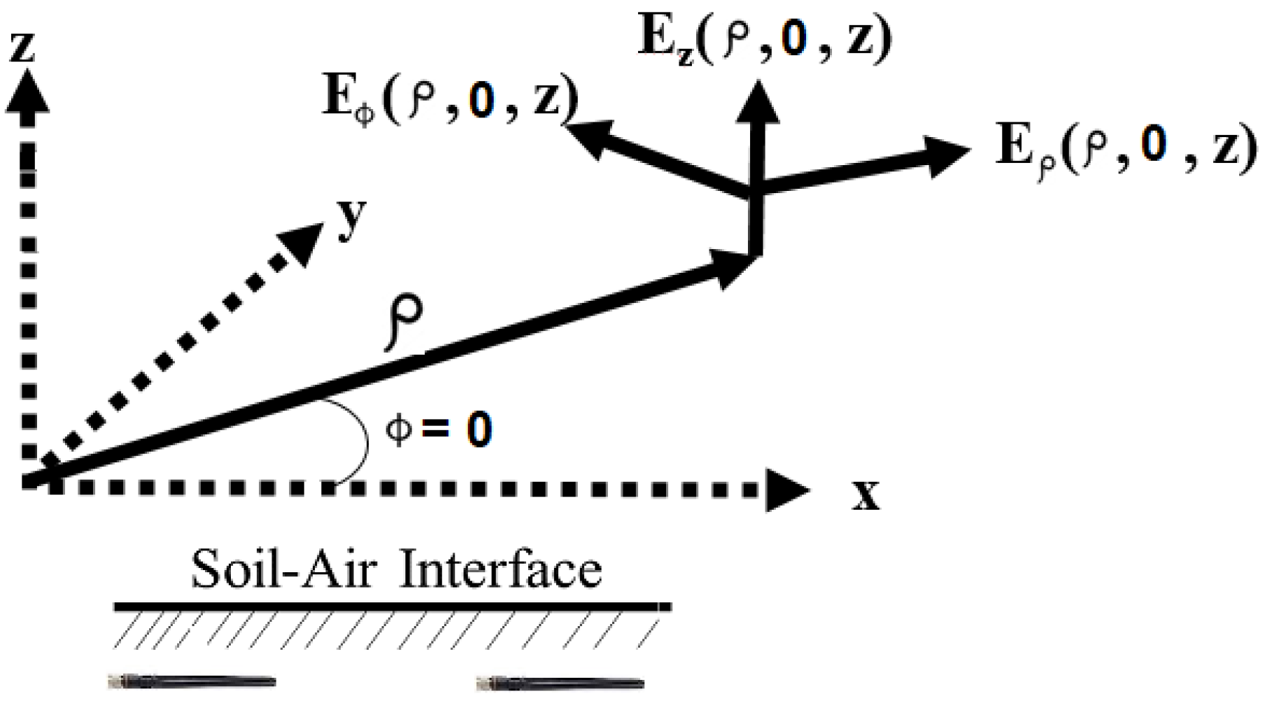
Figure 2.
The coordinates for a lateral wave at the surface, .

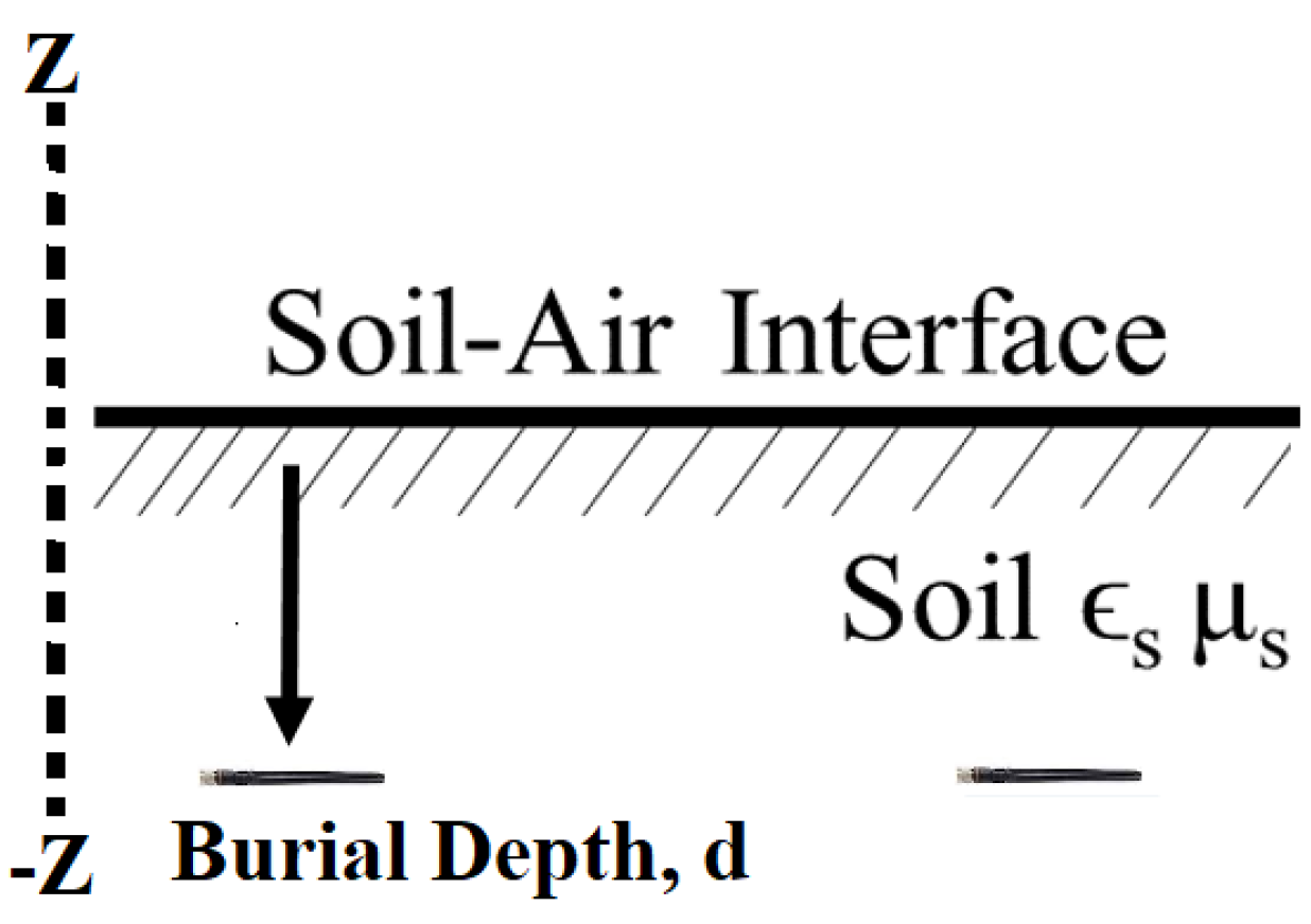
Figure 3.
The burial depth and the z-axis.

Figure 4.
The comparison of the power density of and components at different burial depths: (a) 10-cm depth; (b) 30-cm depth.
Figure 4.
The comparison of the power density of and components at different burial depths: (a) 10-cm depth; (b) 30-cm depth.

Figure 5.
The power density for different burial depths: (a) component; (b) component.

© 2019 by the author. Licensee MDPI, Basel, Switzerland. This article is an open access article distributed under the terms and conditions of the Creative Commons Attribution (CC BY) license (http://creativecommons.org/licenses/by/4.0/).
Share and Cite
MDPI and ACS Style
Salam, A. An Underground Radio Wave Propagation Prediction Model for Digital Agriculture. Information 2019, 10, 147. https://doi.org/10.3390/info10040147
AMA Style
Salam A. An Underground Radio Wave Propagation Prediction Model for Digital Agriculture. Information. 2019; 10(4):147. https://doi.org/10.3390/info10040147
Chicago/Turabian StyleSalam, Abdul. 2019. "An Underground Radio Wave Propagation Prediction Model for Digital Agriculture" Information 10, no. 4: 147. https://doi.org/10.3390/info10040147
Note that from the first issue of 2016, this journal uses article numbers instead of page numbers. See further details here.