A Hybrid Algorithm for Forecasting Financial Time Series Data Based on DBSCAN and SVR


Abstract
:1. Introduction
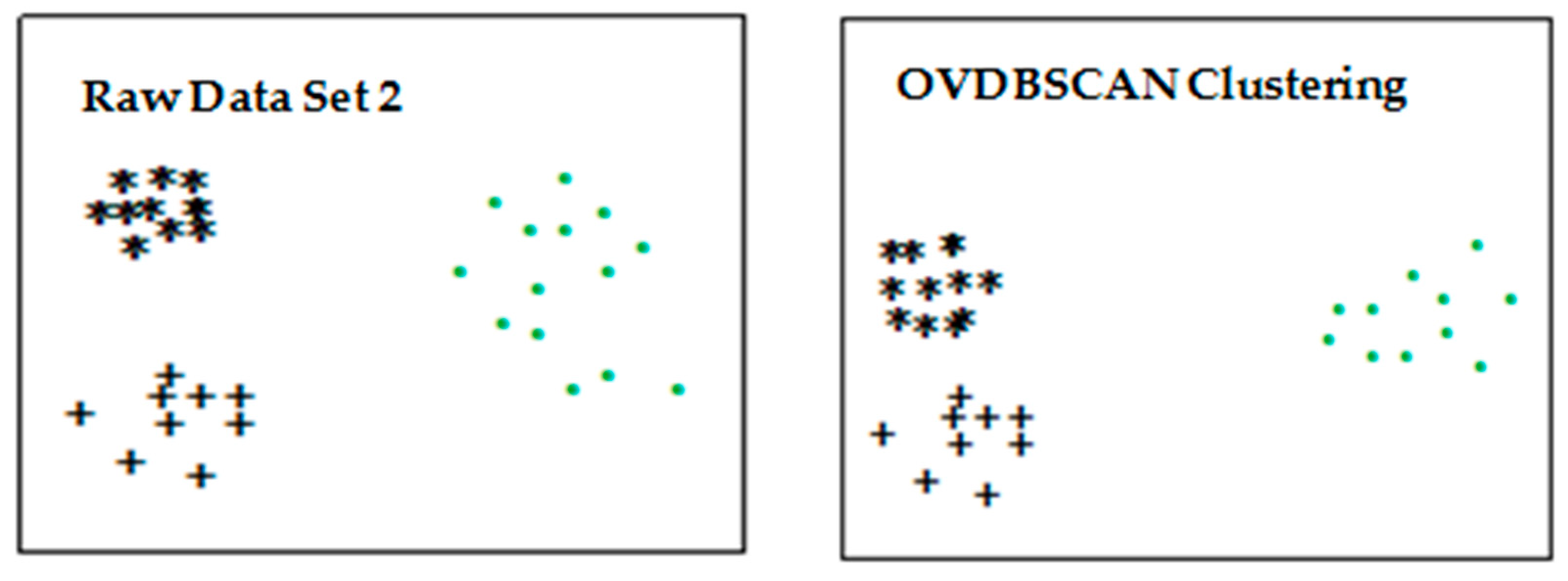
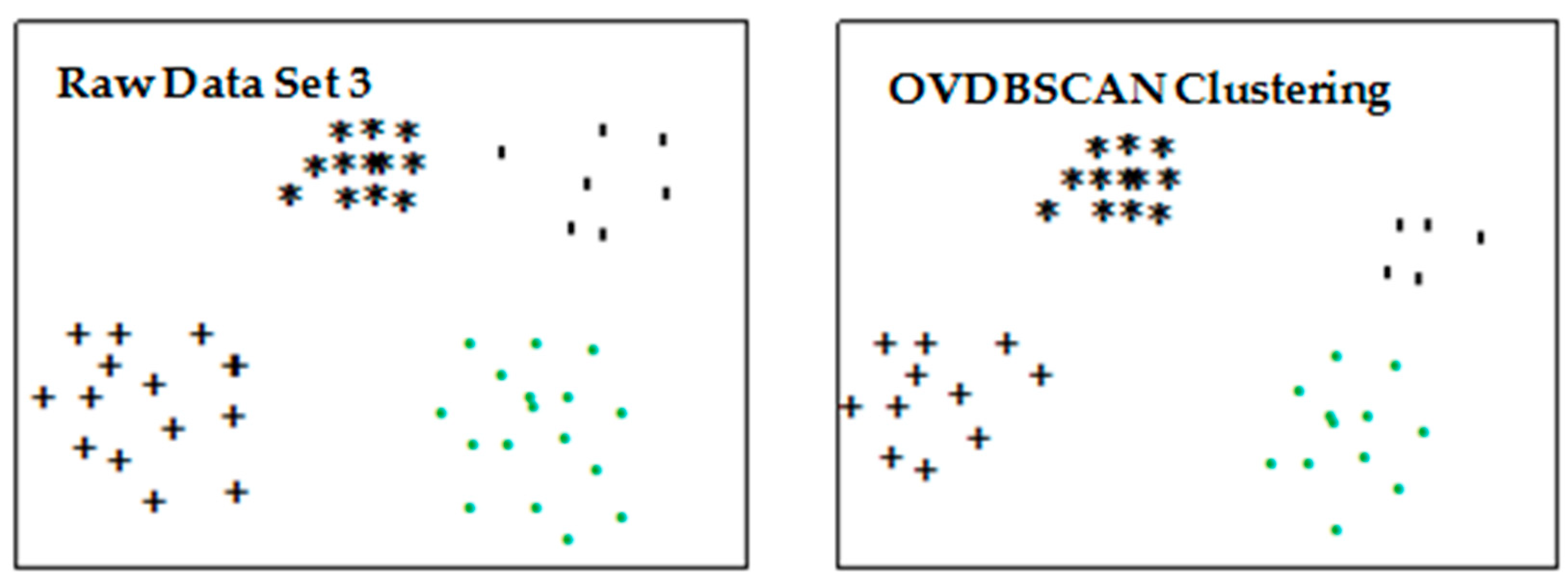
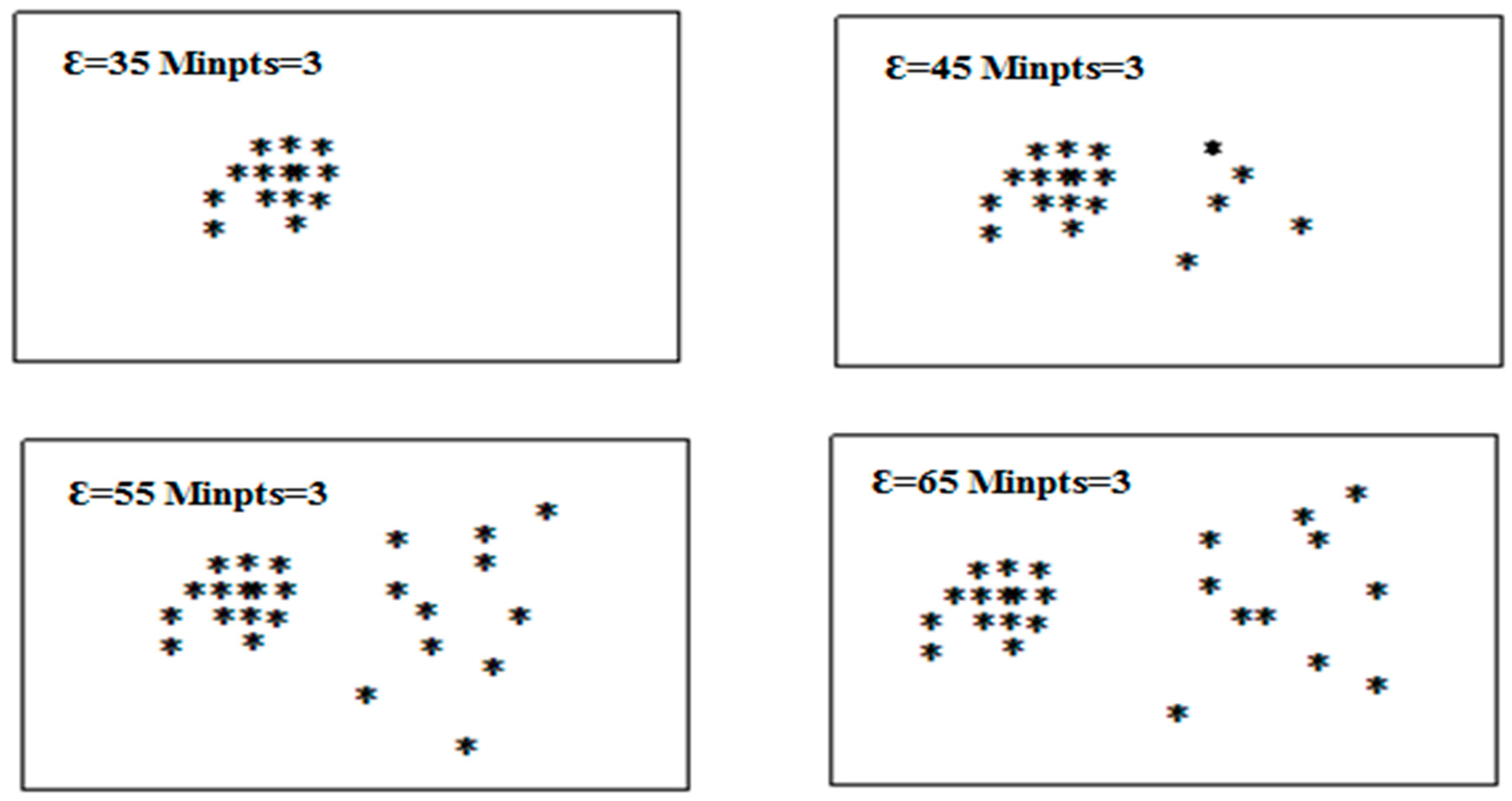
- The parameters of the DBSCAN algorithm are sensitive and global, so it cannot effectively cluster datasets of different densities. This paper proposes an Optimization Initial Points and Variable-Parameter DBSCAN (OVDBSCAN) algorithm based on parameter adaption;
- This paper combines the OVDBSCAN algorithm with SVR and proposes a new “hybridize OVDBSCAN with SVR” (HOS) algorithm. By establishing the regression prediction model, the regression prediction of the unsteady noise data is realized, and the prediction accuracy of stock price and the financial index is improved.
2. Related Work
3. Hybridizing OVDBSCAN with a Support Vector Regression Algorithm
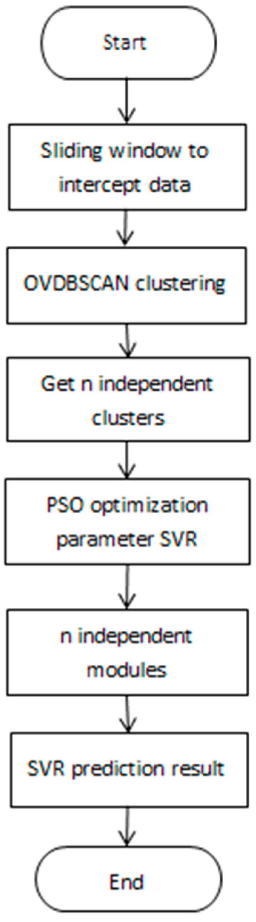
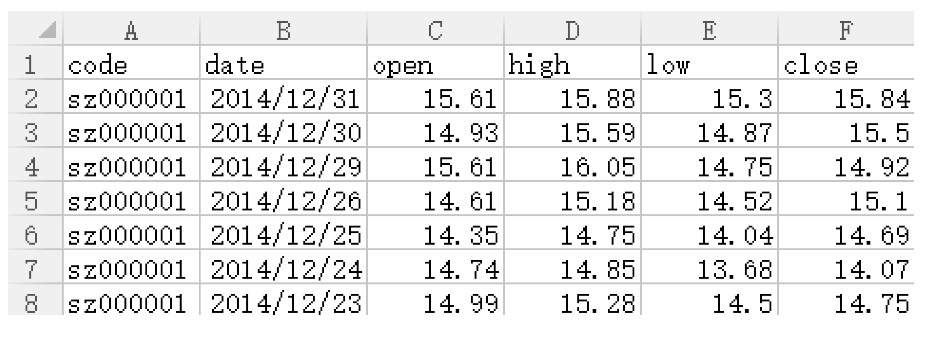
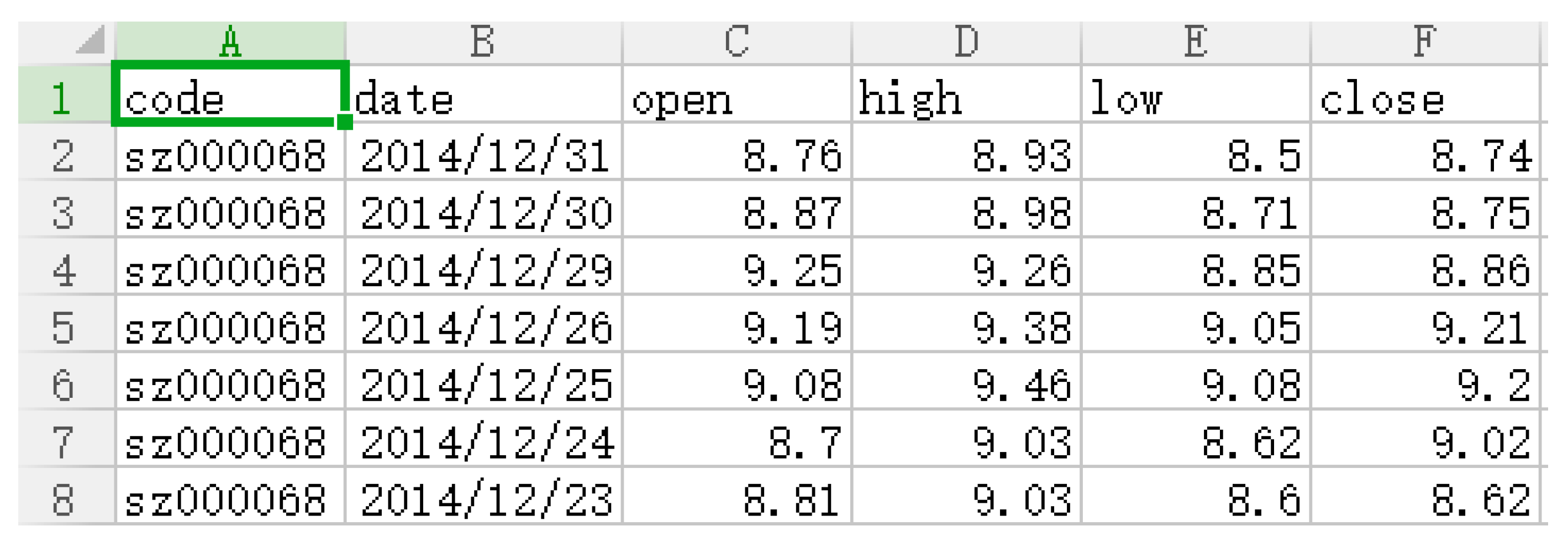
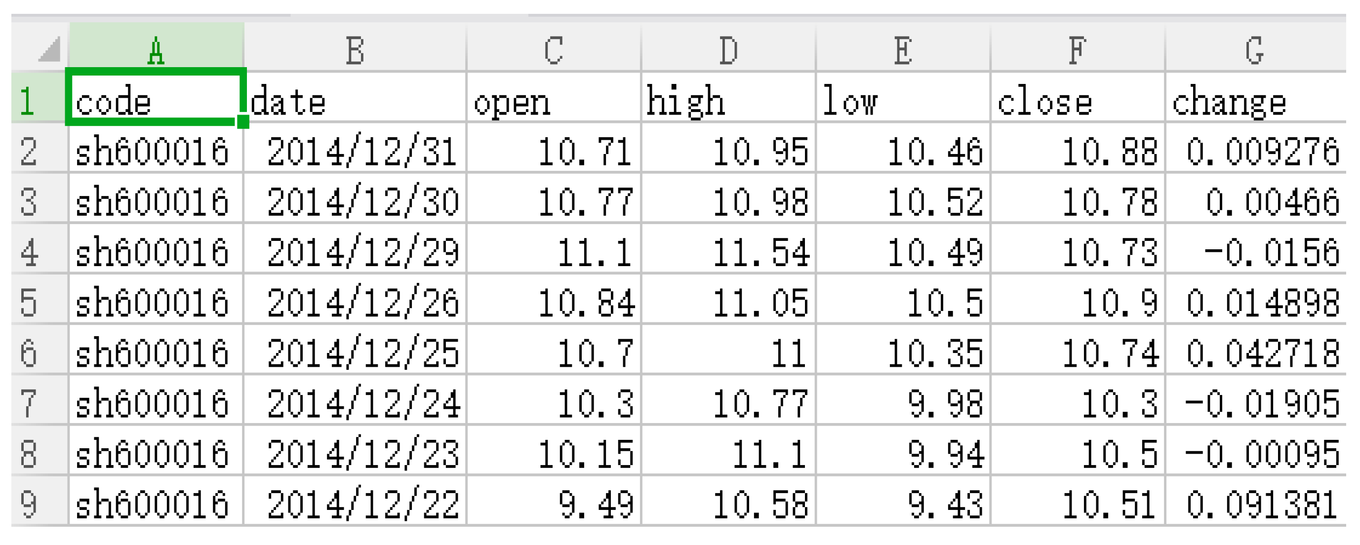
- The width of the sliding window is fixed. The data of n − 1 day are selected as the input data, and the data of the nth day as the output data, so that the data with a span of m years can be mined and studied. The format of the time series data intercepted by the sliding window is as follows, where I is the input sequence, O is the output sequence, x is the n − 1 input data on the nth day, and y is the output data on the nth day:
- There are two basic domain parameters in the OVDBSCAN algorithm: represents the distance threshold of a certain domain, and MinPts represents the number of sample points in the domain with radius First of all, select point p, find the distance of m points closest to point p, and calculate its average value. Then calculate the average distance of m nearest points from all points and store it in the distance_all of the structure. The average distance dataset of all points is clustered through DBSCAN to obtain cps clustering results, and the maximum value of the average distance point is obtained for each class i in cps. Then the distance between p and m closest to it is going to be of that kind of a point. The obtainedis clustered from small to large, and the smallest X is selected. MinPts remains unchanged, and DBSCAN clustering is performed on the dataset. Choose the second smallest until all are used. After clustering, n independent clusters A and their center points will be obtained.
- Model training of -SVR is carried out for n independent clusters A. Since the dataset is nonlinear, SVR introduces the kernel function to solve the nonlinear problem. The expression isThe radial basis function is used to select appropriate parameters, namely the penalty coefficient C, insensitive loss coefficient , and width coefficient , to train the cluster A model. The expression is as follows:
- Cluster , trained by model ε-SVR, is optimized for particle swarm optimization (PSO) parameters: can be set by past experience. Mean square error is obtained by k-fold cross validation:where is the predicted value of .
- After optimizing the parameters, the cluster that was optimized by the parameters is trained, and the model is obtained.
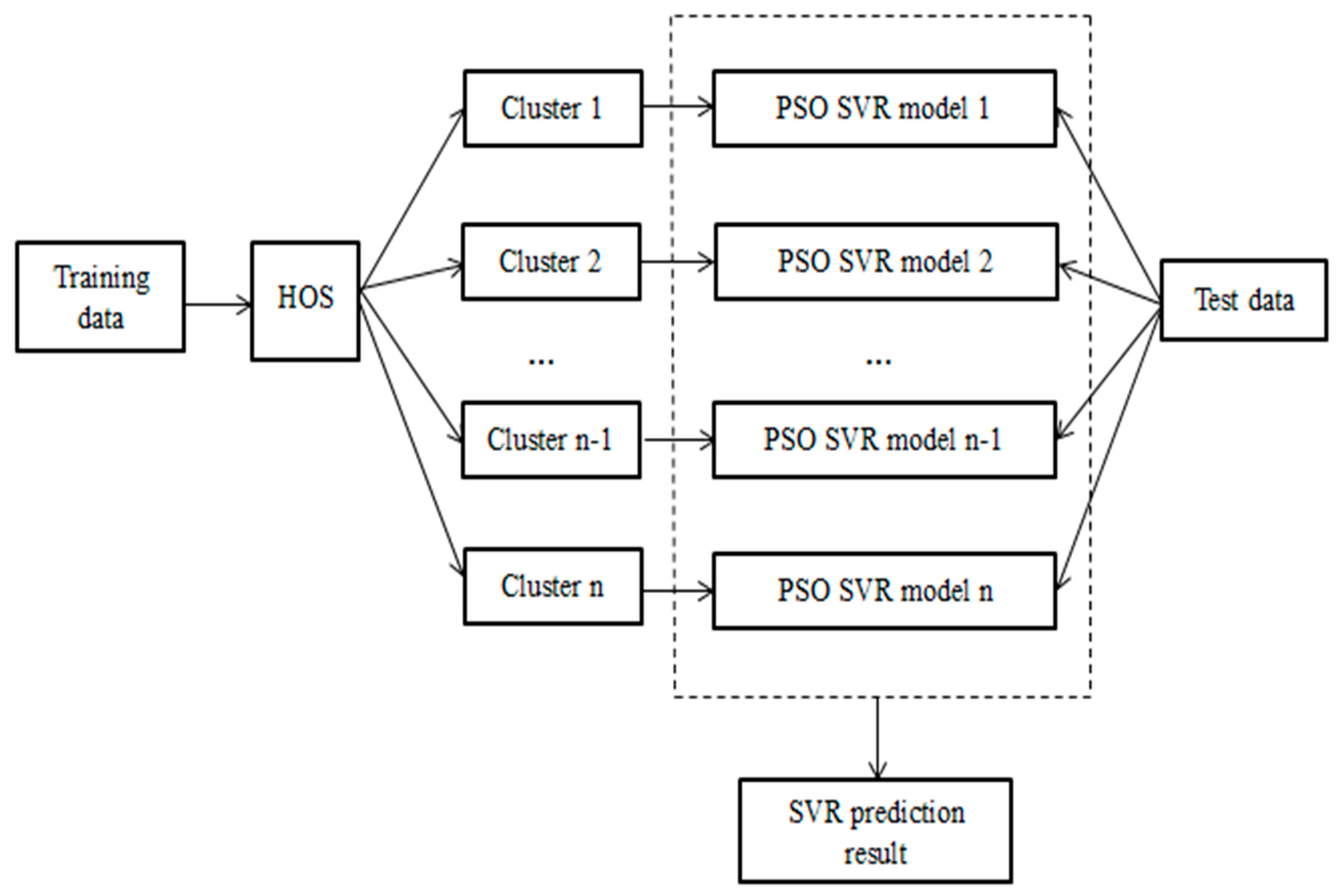
- The test data are matched with n cluster centers after clustering using the DBSCAN algorithm to find the most similar W cluster center and the model M corresponding to the W cluster.
- The predicted value of test data is calculated with the SVR of the corresponding model M. Complete dataset mining and regression analysis.
3.1. DBSCAN Parameter Optimization
- Find the distance of m points closest to P and average them. Find the average distance of m closest points from all points;
- The average distance dataset of m nearest points of all points is clustered through DBSCAN, and cps clustering results are obtained;
- Find the maximum value of the average distance point for each class i in cps;
- The distance between point P and the closest point m to it is the distance of this point.
- The obtained in the above paper is sorted from small to large to start clustering;
- Select the smallest . MinPts remains unchanged. DBSCAN clustering is performed on the dataset;
- Select the second smallest. MinPts remains unchanged. Cluster the data marked as noise;
- Cycle through the above operations until all are used up and the clustering ends.
3.2. PSO Optimization Parameters
3.2.1. Particle Swarm Optimization Principle
3.2.2. PSO to Optimize
- Divide the training data into k parts: , , ..., ;
- Use the current (c,) for training, and obtain mean square error (MSE) by cross-validation;
- Initialize i, and let it equal 1;
- Use as the test dataset and the other as the training set;
- Calculate the MSE of the ith subset. Perform i = i + 1. Return to the fifth step until i = k + 1;
- Calculate the average value of k times of MSE;
- Select the average MSE value after k-fold cross-validation, and record the Pbest and Gbest of individuals and groups. Continue to find better (c, Repeat steps 2 through 8 until the set number of times is satisfied;
- End.
3.3. The Thought of the HOS Algorithm
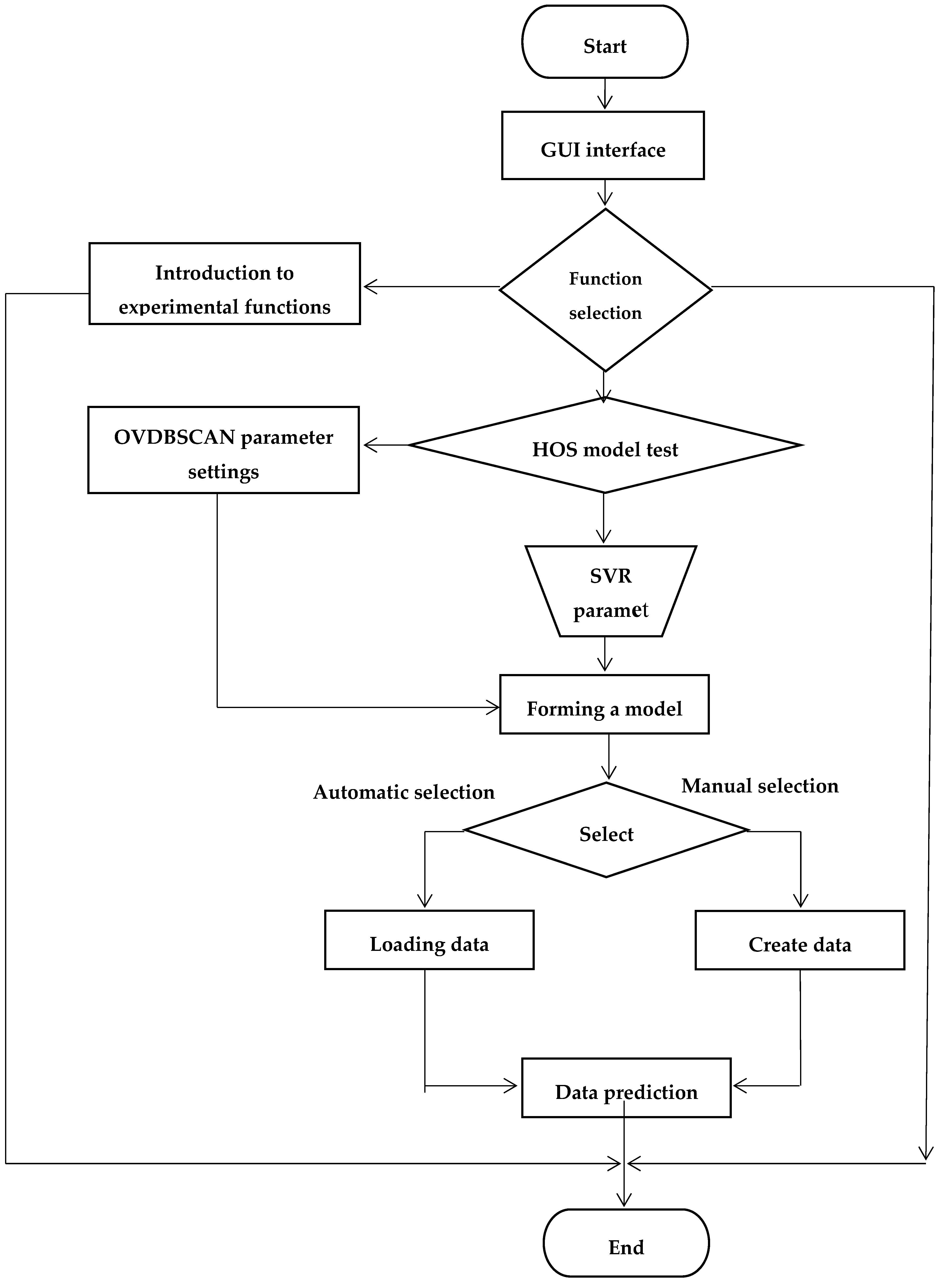
- System interface module;
- Experimental introduction module. Explain the function of each module briefly;
- Experimental module for SVR model design. Implement various functions of SVR (dataset loading, parameter settings, regression demonstration).
4. Research on Financial Time Series Predictions Based on HOS Algorithm
4.1. Optimization of Clustering Algorithm Based on DBSCAN Algorithm
4.1.1. Experimental Design
- = 23.012816, = 78.175813;
- = 27.56658, = 80.039573, = 80.039673;
- = 40.1995502, = 83.743656;
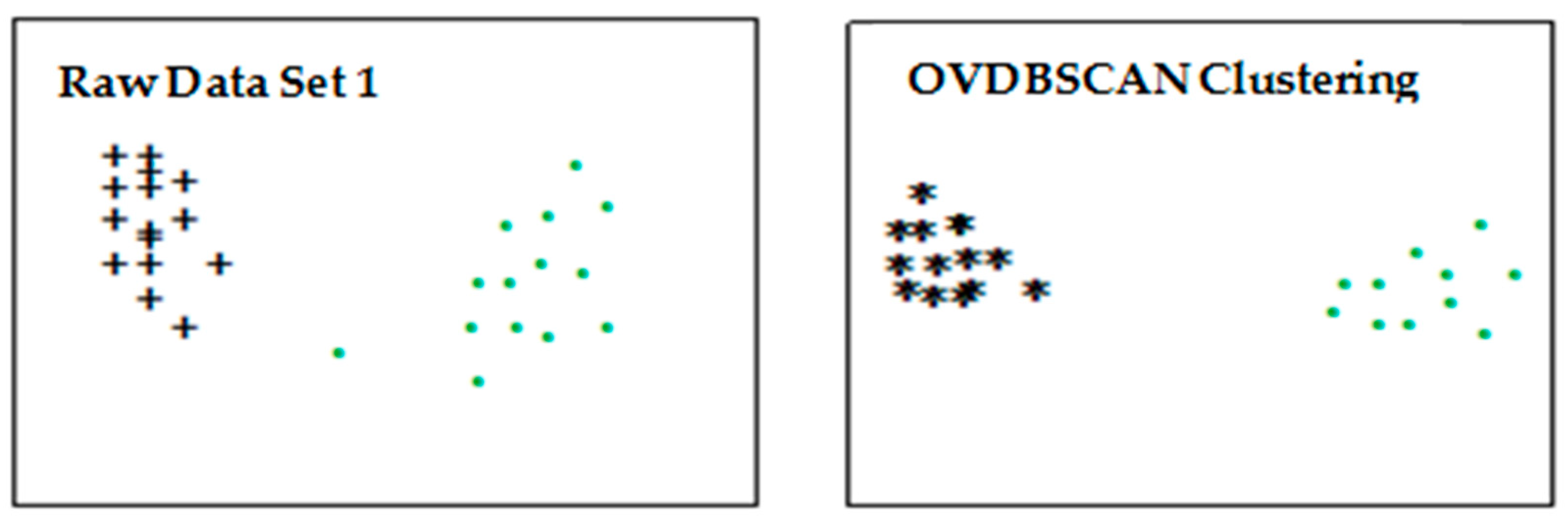
4.1.2. Experimental Results
4.2. Financial Index Prediction Based on HOS Algorithm
4.2.1. Experimental Design
4.2.2. Experimental Results
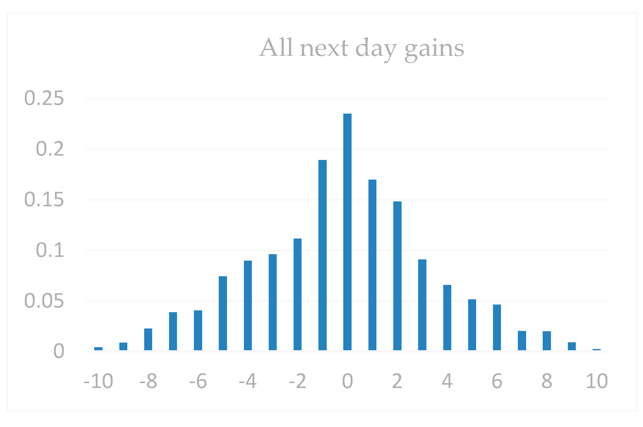
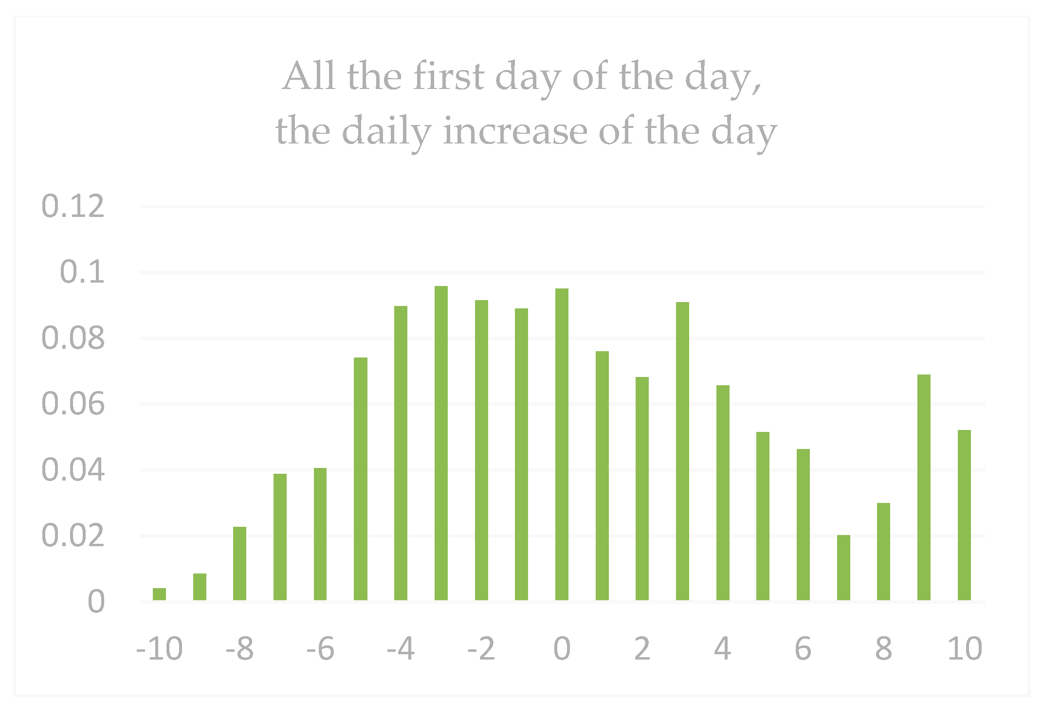
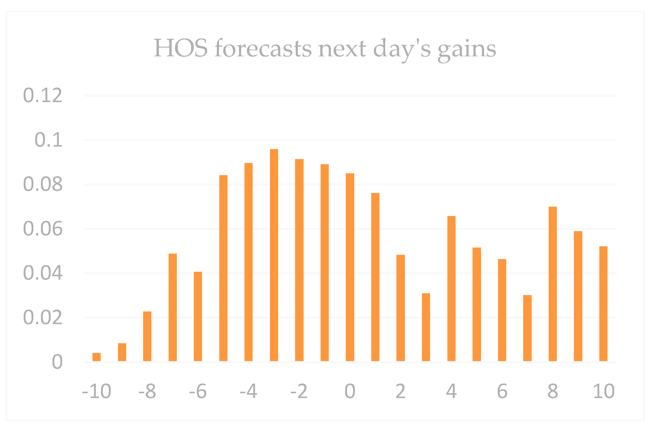
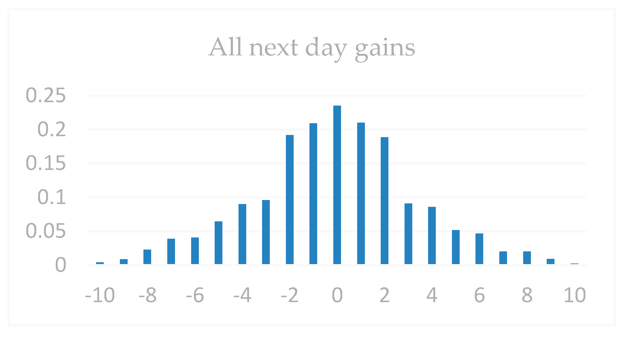
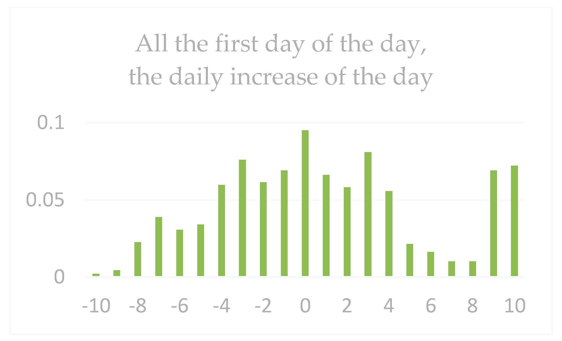
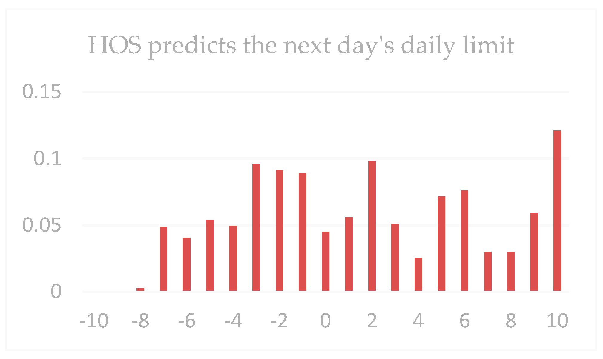
4.3. Prediction of the Next-Day Trading Limit of a Stock Based on the HOS Algorithm
4.3.1. Experimental Design
4.3.2. Experimental Results
4.4. Stock Price Predicting Based on HOS Algorithm
4.4.1. Experimental Design
4.4.2. Experimental Results
5. Conclusions
Author Contributions
Funding
Acknowledgments
Conflicts of Interest
References
- Dablemont, S.; Verleysen, M.; Van Bellegem, S. Modelling and Forecasting financial time series of “tick data”. Forecast. Financ. Mark. 2007, 5, 64–105. [Google Scholar]
- Washio, T.; Shinnou, Y.; Yada, K.; Motoda, H.; Okada, T. Analysis on a Relation Between Enterprise Profit and Financial State by Using Data Mining Techniques. In New Frontiers in Artificial Intelligence; Springer: Berlin/Heidelberg, Germany, 2006. [Google Scholar]
- Yan, L.J. The present situation and future development trend of financial supervision in China. Cina Mark. 2010, 35, 44. [Google Scholar]
- Liao, T.W. Clustering of time series data—A survey. Pattern Recogn. 2005, 38, 1857–1874. [Google Scholar] [CrossRef]
- Rubin, G.D.; Patel, B.N. Financial Forecasting and Stochastic Modeling: Predicting the Impact of Business Decisions. Radiology 2017, 283, 342. [Google Scholar] [CrossRef] [PubMed]
- Qadri, M.; Ahmad, Z.; Ibrahim, J. Potential Use of Data Mining Techniques in Information Technology Consulting Operations. Int. J. Sci. Res. Publ. 2015, 5, 1–4. [Google Scholar]
- Xu, Y.; Ji, G.; Zhang, S. Research and application of chaotic time series prediction based on Empirical Mode Decomposition. In Proceedings of the IEEE Fifth International Conference on Advanced Computational Intelligence, Nanjing, China, 18–20 October 2012. [Google Scholar]
- Ertöz, L.; Steinbach, M.; Kumar, V. Fiding Clusters of Different Sizes, Shapes, and Densities in Noise, High Dimensional Data; SIAM: Philadelphia, PA, USA, 2003. [Google Scholar]
- Li, L.H.; Tian, X.; Yang, H.D. Financial time series prediction based on SVR. Comput. Eng. Appl. 2005, 41, 221–224. [Google Scholar]
- Fu, Z.Q.; Wang, X.F. The DBSCAN algorithm based on variable parameters. Netw. Secur. Technol. Appl. 2018, 8, 34–36. [Google Scholar]
- Li, L.; Xu, S.; An, X.; Zhang, L.D. A Novel Approach to NIR Spectral Quantitative Analysis: Semi-Supervised Least-Squares Support Vector Regression Machine. Spectrosc. Spectr. Anal. 2011, 31, 2702–2705. [Google Scholar]
- Agrawal, R.; Faloutsos, C.; Swami, A. Efficient similarity search in sequence database. In Proceedings of the 4th International Conference on Foundations of Data Organization and Algorithms, Chicago, IL, USA, 13–15 October 1993; Springer: London, UK, 1993; pp. 69–848. [Google Scholar]
- Park, J.; Sriram, T.N. Robust estimation of conditional variance of time series using density power divergences. J. Forecast. 2017, 36, 703–717. [Google Scholar] [CrossRef]
- Rojas, I.; Pomares, H. Time Series Analysis and Forecasting; Springer: Berlin/Heidelberg, Germany, 2016. [Google Scholar]
- Das, G.; Lin, k.; Mannila, H.; Renganathan, G.; Smyth, P. Rule discovery from time series. In Proceedings of the Fourth International Conference on Knowledge Discovery and Data Mining, New York, NY, USA, 27–31 August 1998. [Google Scholar]
- Hsu, S.H.; Hsieh, P.A.; Chih, T.C.; Hsu, K.C. A two-stage architecture for stock price forecasting by integrating self-organizing map and support vector regression. Expert Syst. Appl. 2009, 36, 7947–7951. [Google Scholar] [CrossRef] [Green Version]
- Huang, C.L.; Tsai, C.Y. A hybrid SOFM-SVR with a filter-based feature selection for stock market forecasting. Expert Syst. Appl. 2009, 36, 1529–1539. [Google Scholar] [CrossRef]
- Zhang, G.P. Time series forecasting using a hybrid ARIMA and neural network model. Neurocomputing 2003, 50, 159–175. [Google Scholar] [CrossRef]
- Folkes, S.R.; Lahav, O.; Maddox, S.J. An artificial neural network approach to the classification of galaxy spectra. Mon. Not. R. Astron. Soc. 2018, 283, 651–665. [Google Scholar] [CrossRef]
- Tang, J.H. A review on the nonlinear time series model of regularly sampled data. Math. Progress 1989, 18, 22–43. [Google Scholar]
- Xiong, Z.F. Wavelet Method for Fractal Dimension Estimation of Financial Time Series. Syst. Eng. Theory Pract. 2002, 22, 48–53. [Google Scholar]
- Xu, M.; Huang, C. Financial Benefit Analysis and Forecast Based on Symbolic Time Series Method. CMS 2011, 19, 1–9. [Google Scholar]
- Li, B.; Zhang, J.P.; Liu, X.J. Time-series Detection of Uncertain Anomalies Based on Hadoop. Chin. J. Sens. Actuators 2015, 7, 1066–1072. [Google Scholar]
- Box, G.E.P.; Jenkins, G.M. Time Series Analysis: Forecasting and Control. J. Time 2010, 31, 303. [Google Scholar]
- Xi, L.; Muzhou, H.; Lee, M.H.; Li, J.; Wei, D.; Hai, H.; Wu, Y. A new constructive neural network method for noise processing and its application on stock market prediction. Appl. Soft Comput. 2014, 15, 57–66. [Google Scholar] [CrossRef]
- Kumar, K.M.; Reddy, A.R.M. A fast DBSCAN clustering algorithm by accelerating neighbor searching using Groups method. Pattern Recognit. 2016, 58, 39–48. [Google Scholar] [CrossRef]
- Limwattanapibool, O.; Arch-Int, S. Determination of the appropriate parameters for K-means clustering using selection of region clusters based on density DBSCAN (SRCD-DBSCAN). Expert Syst. 2017, 34, e12204. [Google Scholar] [CrossRef]
- Wang, F.S.; Chen, L.H. Particle Swarm Optimization (PSO); Springer: Berlin/Heidelberg, Germany, 2013. [Google Scholar]
- Gou, J.; Lei, Y.X.; Guo, W.P.; Wang, C.; Cai, Y.Q.; Luo, W. A novel improved particle swarm optimization algorithm based on individual difference evolution. Appl. Soft Comput. 2017, 57, 468–481. [Google Scholar] [CrossRef]
- Shah, G.H. An improved DBSCAN, a density based clustering algorithm with parameter selection for high dimensional data sets. In Proceedings of the Nirma University International Conference on Engineering, Ahmedabad, India, 28–30 November 2013. [Google Scholar]
- Wei, W.; Jiang, J.; Liang, H.; Gao, L.; Liang, B.; Huang, J.; Zang, N.; Liao, Y.; Yu, J.; Lai, J.; et al. Application of a Combined Model with Autoregressive Integrated Moving Average (ARIMA) and Generalized Regression Neural Network (GRNN) in Forecasting Hepatitis Incidence in Heng County, China. PLoS ONE 2016, 11, e0156768. [Google Scholar] [CrossRef] [PubMed]
- Wu, H.; Cai, Y.; Wu, Y.; Zhong, R.; Li, Q.; Zheng, J.; Lin, D.; Li, Y. Time series analysis of weekly influenza-like illness rate using a one-year period of factors in random forest regression. BioSci. Trends 2017, 11, 292–296. [Google Scholar] [CrossRef] [PubMed]
- Lodwick, W.A.; Jamison, K.D. A computational method for fuzzy optimization. In Uncertainty Analysis in Engineering and Sciences: Fuzzy Logic, Statistics and Neural Network Approach; Avvub, B.M., Guota, M.M., Eds.; Kluwer Academic Publisher: Boston, MA, USA, 1998. [Google Scholar]


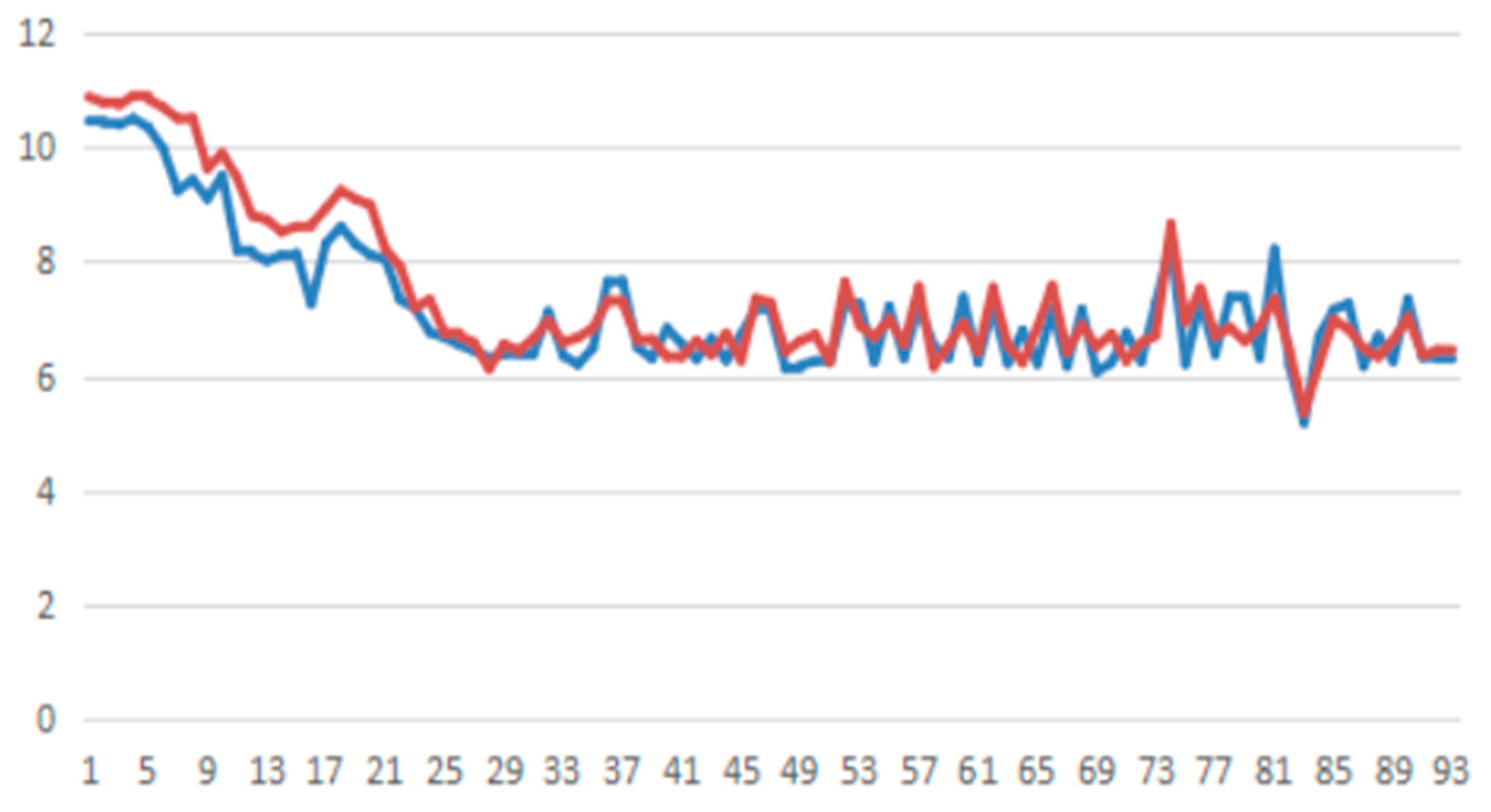
 actual value
  predicted value).
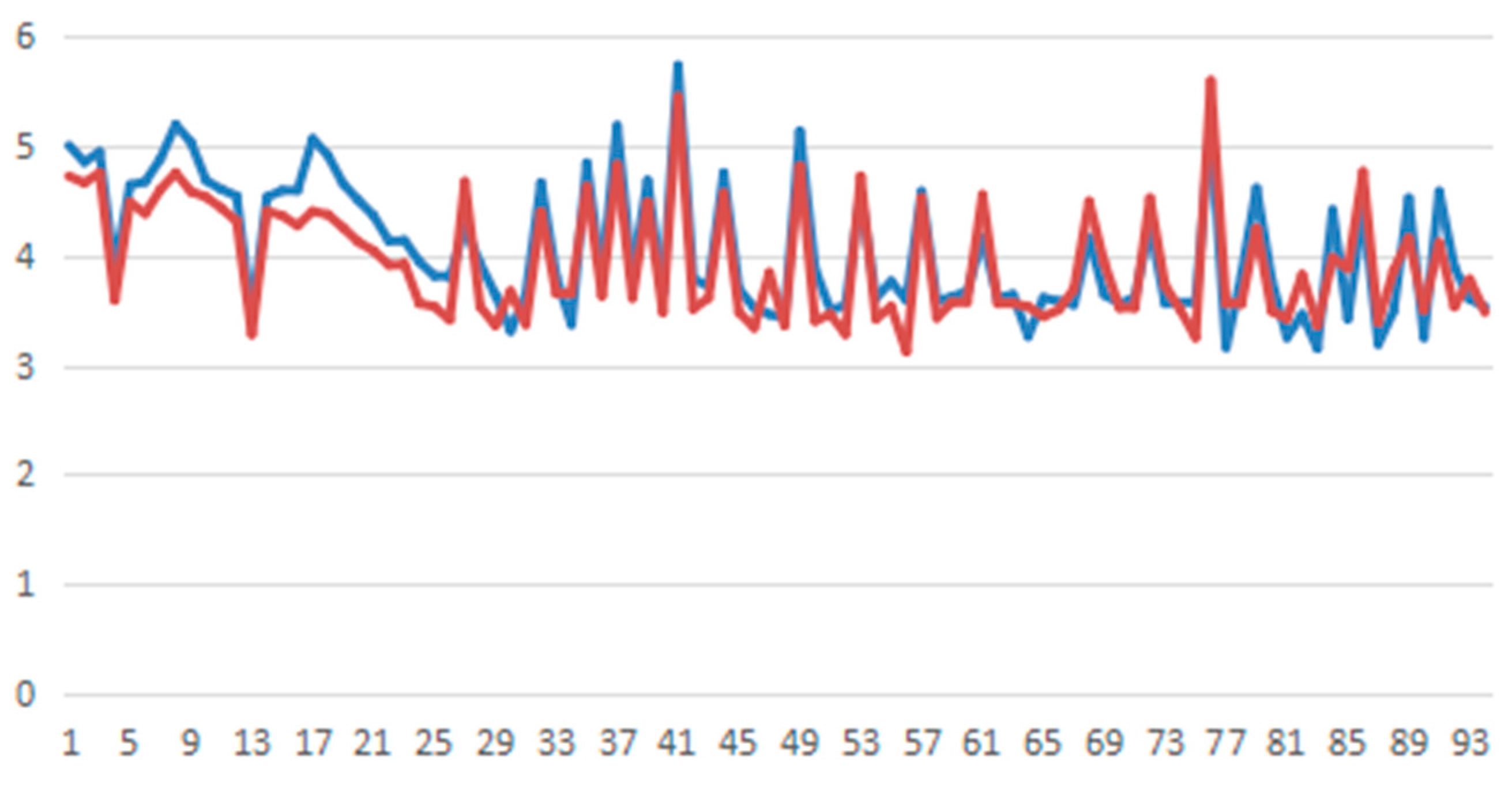
 actual value
  predicted value).

| Packet Number | Training Data | Test Data |
|---|---|---|
| 1 | 2013.1.4–2014.4.4 | 2014.4.5–2014.9.4 |
| 2 | 2013.2.4–2014.5.4 | 2014.5.5–2014.10.4 |
| 3 | 2013.3.4–2014.6.4 | 2014.6.5–2014.11.4 |
| 4 | 2013.4.4–2014.7.4 | 2013.7.5–2014.12.31 |
| HOS | Numerical Value | SVR | Numerical Value | PSO | Numerical Value |
|---|---|---|---|---|---|
| k | 25 | Maximum value of c | 100 | Local search capability | 1.5 |
| cps | 2000 | Maximum value of c | 0.01 | Global search capability | 1.7 |
| Maximum value of | 1000 | Maximum evolutionary quantity | 200 | ||
| Maximum value of | 0.01 | Maximum population value | 20 | ||
| 0.01 | Cross-validation k | 5 |
| Dataset | MSE | MAE | MAPE |
|---|---|---|---|
| 1 | 4567 | 53.62 | 0.7318 |
| 2 | 5926 | 59.38 | 0.9637 |
| 3 | 4857 | 58.16 | 0.9368 |
| 4 | 3598 | 48.71 | 0.6862 |
| Dataset | MSE | MAE | MAPE |
|---|---|---|---|
| 1 | 27,853 | 163.12 | 2.7518 |
| 2 | 365,819 | 429.68 | 6.3294 |
| 3 | 13,829 | 265.42 | 3.5291 |
| 4 | 21,964 | 103.55 | 2.1372 |
| Dataset | MSE | MAE | MAPE |
|---|---|---|---|
| 1 | 26,197 | 153.28 | 2.2275 |
| 2 | 48,392 | 162.53 | 2.5296 |
| 3 | 8375 | 68.97 | 1.3625 |
| 4 | 19,374 | 77.82 | 1.6482 |
| Dataset Number | Training Data | Test Data |
|---|---|---|
| 1 | 2013.01.04–2014.8.31 | 2014.9.01–2014.11.31 |
| 2 | 2013.01.04–2014.9.30 | 2014.10.01–1014.12.31 |
| Dataset 1 | Gain < −9 | Gain < −5 | Gain < −3 | Gain > 0 | Gain > 3 | Gain > 5 | Gain > 9 |
|---|---|---|---|---|---|---|---|
| All next-day gains | 0.57 | 4.62 | 11.86 | 48.37 | 9.06 | 4.35 | 1.3 |
| All the first daily limits | 2.08 | 7.32 | 13.57 | 62.52 | 35.95 | 22.73 | 12.66 |
| HOS | 1.03 | 10.0 | 17.92 | 60.39 | 37.62 | 23.83 | 16.18 |
| Dataset 2 | Gain < −9 | Gain < −5 | Gain < −3 | Gain > 0 | Gain > 3 | Gain > 5 | Gain > 9 |
|---|---|---|---|---|---|---|---|
| All next-day gains | 0.38 | 1.69 | 6.97 | 57.25 | 15.03 | 5.75 | 1.58 |
| All the first daily limits | 0.26 | 2.21 | 11.06 | 66.82 | 39.97 | 25.41 | 13.05 |
| HOS | 0 | 1.58 | 7.89 | 71.02 | 46.35 | 38.07 | 17.01 |
| Data Source | Training Data | Test Data |
|---|---|---|
| Minsheng Bank | 2013.1.4–2014.8.15 | 2014.8.16–2014.12.31 |
| China Unicom | 2013.1.4–2014.8.15 | 2014.8.16–2014.12.31 |
© 2019 by the authors. Licensee MDPI, Basel, Switzerland. This article is an open access article distributed under the terms and conditions of the Creative Commons Attribution (CC BY) license (http://creativecommons.org/licenses/by/4.0/).
Share and Cite
Huang, M.; Bao, Q.; Zhang, Y.; Feng, W. A Hybrid Algorithm for Forecasting Financial Time Series Data Based on DBSCAN and SVR. Information 2019, 10, 103. https://doi.org/10.3390/info10030103
Huang M, Bao Q, Zhang Y, Feng W. A Hybrid Algorithm for Forecasting Financial Time Series Data Based on DBSCAN and SVR. Information. 2019; 10(3):103. https://doi.org/10.3390/info10030103
Chicago/Turabian StyleHuang, Mengxing, Qili Bao, Yu Zhang, and Wenlong Feng. 2019. "A Hybrid Algorithm for Forecasting Financial Time Series Data Based on DBSCAN and SVR" Information 10, no. 3: 103. https://doi.org/10.3390/info10030103
APA StyleHuang, M., Bao, Q., Zhang, Y., & Feng, W. (2019). A Hybrid Algorithm for Forecasting Financial Time Series Data Based on DBSCAN and SVR. Information, 10(3), 103. https://doi.org/10.3390/info10030103