Object Recognition Using Non-Negative Matrix Factorization with Sparseness Constraint and Neural Network

Abstract

UAVs (unmanned aerial vehicles) have been widely used in many fields, where they need to be detected and controlled. Small-sample UAV recognition requires an effective detecting and recognition method. When identifying a UAV target using the backward propagation (BP) neural network, fully connected neurons of BP neural network and the high-dimensional input features will generate too many weights for training, induce complex network structure, and poor recognition performance. In this paper, a novel recognition method based on non-negative matrix factorization (NMF) with sparseness constraint feature dimension reduction and BP neural network is proposed for the above difficulties. The Edgeboxes are used for candidate regions and Log-Gabor features are extracted in candidate target regions. In order to avoid the complexity of the matrix operation with the high-dimensional Log-Gabor features, preprocessing for feature reduction by downsampling is adopted, which makes the NMF fast and the feature discriminative. The classifier is trained by neural network with the feature of dimension reduction. The experimental results show that the method is better than the traditional methods of dimension reduction, such as PCA (principal component analysis), FLD (Fisher linear discrimination), LPP (locality preserving projection), and KLPP (kernel locality preserving projection), and can identify the UAV target quickly and accurately.

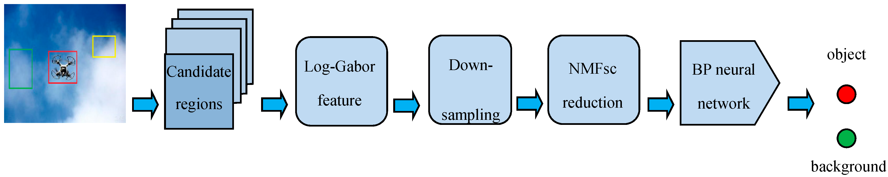
1. Introduction

UAVs (unmanned aerial vehicles) have been widely used in the military and civilian fields in recent years because of their advantages of small size, low cost, low noise, strong maneuverability, high concealment, and superior stability. They can be applied to enemy investigation, dangerous area detection, target tracking, electronic interference, communication relay, and even small-sized weapons. Therefore, it is necessary to detect and monitor non-cooperative UAVs using our UAVs in the air. Through monitoring the border area and other national troops by UAVs in real-time, the border surveillance of wide areas can be realized economical, and it plays a certain security role for the country and society.

It is difficult to identify UAVs because of the variety in illumination, shapes, scales, attitudes, and background in the air. Considering the possibility that the UAV could be hovering in air, the detection method for static images is suitable for UAV targets. We need a fast and effective method to detect targets in a static image. The region proposal method is the first and foremost in importance, while traditional time-consuming sliding window method is not advisable. As can be seen from the following state, the EdgeBoxes method is faster and more accurate than other methods. We select the EdgeBoxes method to extract the region of interest, as it satisfies the real-time requirement.

As for recognition, BP (back propagation) neural network can approximate any nonlinear function. It has many advantages, such as strong ability for suppressing noise, fault tolerance, adaptive learning and parallel processing ability [1,2,3]. It is widely used in the field of target detection. The convolutional neural network of deep learning has achieved excellent results in the field of object detection, however, it needs a large number of data samples to train the network of deep learning. In actual work, such as the UAV object recognition in this paper, it is too difficult to get so many training samples, and it would be easy to overfit under the conditions of limited/few datasets. According to this problem, designing a kind of object recognition method using back propagation neural network is necessary for small sample UAV recognition.

Compared with convolutional neural networks, the back propagation neural network has a short training time and can adapt to environmental change. The accuracy of recognition can meet most of the application requirements [4,5,6,7]. However, when BP neural network is used for UAV target recognition, the high-dimensional input feature makes the network structure complex and reduces training performance, so it is necessary to reduce the original high-dimensional feature before training classifier.

The commonly used methods of feature reduction include principal component analysis (PCA), Fisher linear discriminant analysis (FLD), locality preserving projection (LPP), and so on. The principal component analysis method is simple and efficient, but it is not suitable for high-dimensional nonlinear data structure [8]. Locality preserving projection (LPP) not only solves the problem that in the linear method it is difficult to maintain the nonlinear manifold of the data, but also overcomes the shortcoming that in the nonlinear method it is difficult to obtain the low-dimension projection of new samples. LPP has a good local discriminant ability [9]. The kernel local preserving projection (KLPP) maps the low-dimensional, linear, and inseparable data into high-dimensional space through the kernel function, and has a better ability to extract nonlinear feature than LPP [10]. However, LPP is an unsupervised learning method. When the illumination and attitude of the target change, or the two classes are close and even overlapped, the recognition rate will decline. The process of matrix transforming to vector is easy to bring a dimensionality curse for LPP method, and the amount of calculation is very large.

Non-negative matrix factorization (NMF) is a dimension-reduction technique based on a low-rank approximation of the feature space. Besides providing a reduction in the number of features, NMF guarantees that the features are non-negative, producing additive models that respect, for example, the non-negativity of physical quantities [11]. One of the most useful properties of NMF is that it usually produces a sparse representation of the data. Such a representation encodes much of the data using few ‘active’ components, which makes the encoding easy to interpret. The sparse representation can inhibit the effects of the occlusion, illumination variation, and rotation for feature extraction.

Therefore, a novel UAV target recognition method, based on NMF with sparseness constraint (NMFsc) [12] feature dimension reduction and BP neural network, is proposed in this paper. The Log-Gabor features are extracted from the UAV target image in the first, and then the high-dimensional Log-Gabor features are reduced by the NMFsc algorithm. The BP neural network classifier is used to training and recognition after feature reduction. Compared with PCA (principal component analysis), FLD (Fisher linear discrimination), LPP (locality preserving projection), and KLPP (kernel locality preserving projection), and other algorithms, the method of NMFsc with BP neural network overcomes the problem of both working in real-time and accuracy, and improves the recognition performance. Figure 1 is the flowchart of our algorithm.

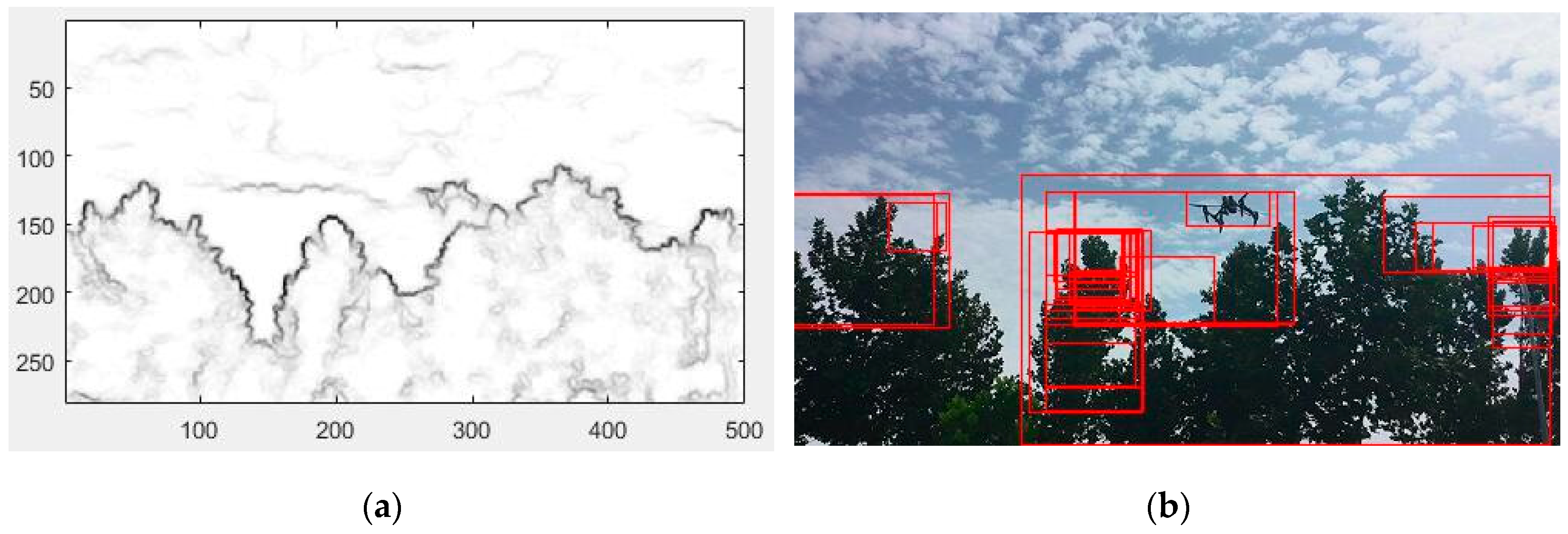
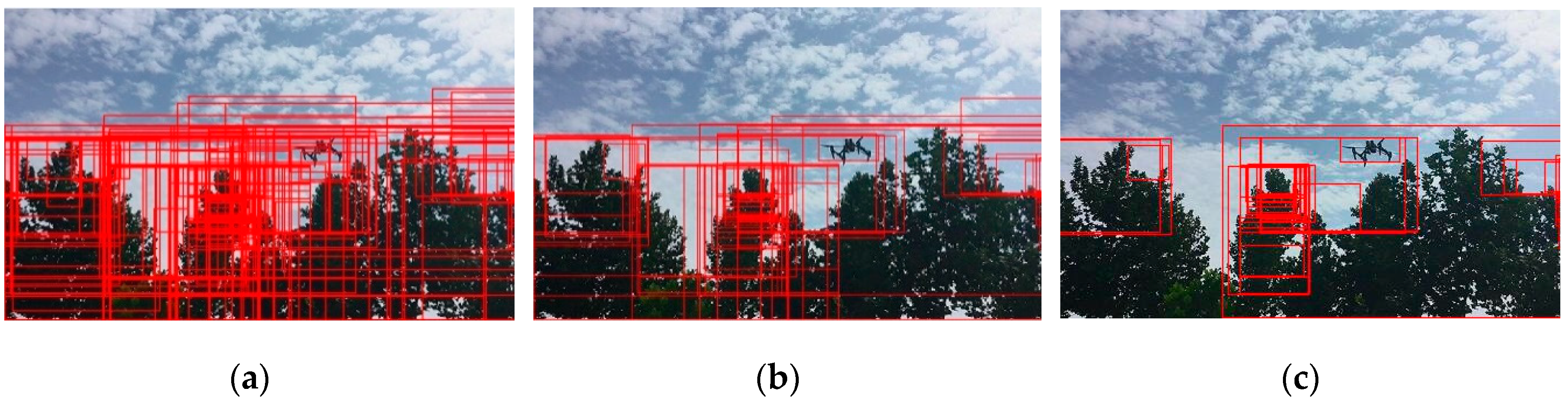
2. UAV Interesting Candidate Regions: Generation and Selection

2.1. Related Algorithms of Region Proposal

These proposal algorithms are broadly divided into two categories: grouping methods and window scoring methods. Grouping methods generate multiple segments of an image which are likely to contain objects. The most common approach to grouping methods is to do hierarchical image segmentation and merge segments according to the similarities between those segments. Most grouping algorithm performance relies on initial segmentation algorithms.

The SelectiveSearch [13] proposal method is one of the well-known methods. SelectiveSearch is based on multiple hierarchical segmentation using superpixels. SelectiveSearch has been broadly used as the proposal method of choice by many state-of-the-art object detectors, including the R-CNN [14] and Fast R-CNN [15] detectors. For covering a diverse set of regions, different kinds of grouping strategies and color spaces are used, which produce high recall at fast speeds—a few seconds per image. However, there is no scoring mechanism on the proposals; therefore, proposals cannot be ranked. Carreira and Sminchisescu [16], CMPC, and Endres and Hoiem [17] methods solve multiple graph cuts with different seeds and parameters to generate class-independent proposals. Both of these methods generate binary foreground/background segments, with each obtained foreground segment as an object hypothesis, and both of these methods learn to predict the segments that cover complete objects and rank proposals accordingly. However, both algorithms are slow due to their reliance on the gPb edge detector, but generate high-quality segmentation masks.

On the other hand, window scoring methods are very different, with each window score being calculated according to how likely it is to contain an object. This approach generates a bounding box much faster than the grouping methods. However, this approach has low localization accuracy. Objectness [18] is a window-based approach in which each candidate window score is calculated according to different image cues. This method uses saliency, color contrast, edge density, and superpixel straddling cues to obtain the characteristics of images, and adopts Bayesian’s framework to combine several cues. The last advantage of objectness is its slow emergence of drawback, which appears at a snail’s speed. This method has low localization accuracy, but the first few proposals it obtains are of high quality.

Rahtu et al. [19] begins with a large number of randomly sampled boxes from an objectness and multiplies them with proposal regions generated from single, pair, and triplet superpixel segmentations.

EdgeBoxes [20] is another window-based approach, and is among the fastest object proposal generation methods. EdgeBoxes generates object proposals directly from the edges of an image.

Table 1. Comparison of different region proposal methods.

Method	Approach	Time (s)	Recall Results	Detection Results
SelectiveSearch [13]	Grouping	10	***	***
Rantalankila [22]	Grouping	10	·	**
CPMC [16]	Grouping	250	**	*
Endres and Hoiem [17]	Grouping	100	***	**
Objectness [18]	Window scoring	3	*	·
Rahtu [19]	Window scoring	3	·	*
EdgeBoxes [20]	Window scoring	0.3	***	***
Bing [21]	Window scoring	0.2	*	·

·, *, **, *** indicate progressively better results.

shows results of the different approaches. The EdgeBoxes approach is significantly faster and more accurate than previous approaches. The only methods with comparable accuracy are SelectiveSearch and CPMC, but these are considerably slower. The only method with comparable speed is BING [21], but BING has the worst accuracy of all evaluated methods at IoU of 0.7 [20].

2.2. UAV Interesting Candidate Regions Selection

Through the analysis above, the EdgeBoxes method has good performance in speed and accuracy. We select the EdgeBoxes method to obtain the interesting candidate regions. As the UAV might hover in the air, we detect and identify the UAV target in static images. The 0.2 s region proposal time satisfies practical requirement. The image effect of EdgeBoxes method is shown in Figure 2.

3. Feature Extraction and Dimension Reduction

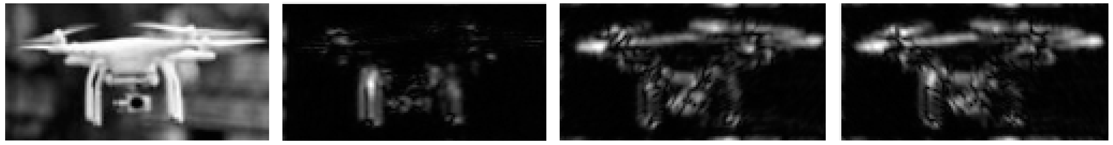
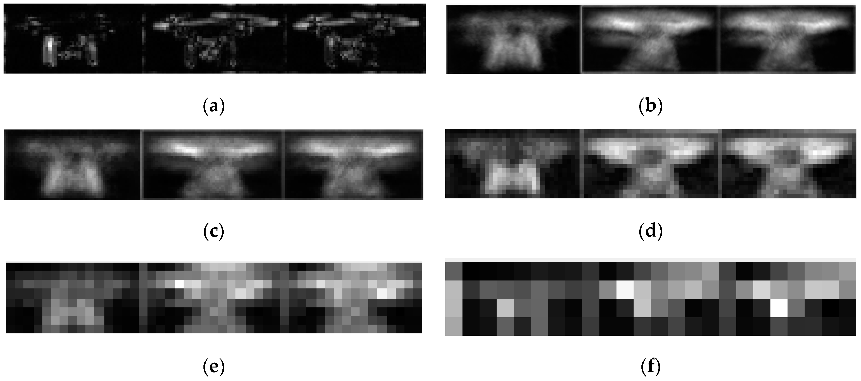
3.1. Log-Gabor Feature Extraction

Field proposes an alternate method to perform both the DC compensation and to overcome the bandwidth limitation of a traditional Gabor filter. The Log-Gabor filter has a response that is Gaussian when viewed on a logarithmic frequency scale instead of a linear one. This allows more information to be captured in the high frequency areas and also has desirable high pass characteristics.

Log-Gabor filters in frequency domain can be defined in polar coordinates by H (f, θ) = H_f × H_θ, where H_f is the radial component and H_θ, the angular one:

$$H(f,\theta )=\exp \left\{\frac{-{[\ln (f/f_0)]}^2}{2{[\ln ({\sigma }_f/f_0)]}^2}\right\}\times \exp \left\{\frac{-{(\theta -{\theta }_0)}^2}{2{\sigma }_{\theta }^2}\right\}$$

(1)

where f₀ is the central frequency; θ₀, the filter direction; σ_f defines the radial bandwidth; and σ_θ defines the angular bandwidth. In order to maintain constant shape ratio filters, the ratio of σ_f/f₀ should be maintained constant. In the following experiments, the shape parameter is chosen such that each filter has a bandwidth of approximately 2 octaves and the filter bank was constructed with a total of 8 orientations and 5 scales.

Amplitude of Log-Gabor shows the local energy spectrum of image, and it should be regarded as the intensity of edge of specific orientation.

UAV image is filtered by Log-Gabor to extract features. This is an image convolution operation, as follows:

$$L{G}_{u,v}(x,y)=E(x,y)\ast {\mathsf{\Phi }}_{u,v}(x,y)$$

(2)

where * expresses convolution operation, E (x, y) is the UAV image, and Φ_u,v (x, y) is a Log-Gabor filter with u scales and v orientations. LG_u,v (x, y) is the result of convolution operation. Generally, amplitude will be selected.

In order to improve the computing speed of filtering and convolution, the scale and orientation of filter are selected as 1 and 3 separately. The parameters are empirically selected, which σ_θ is 1.5 and σ_f/f₀ is 0.65. Figure 3 shows the convolution result of UAV with one scale and three orientations.

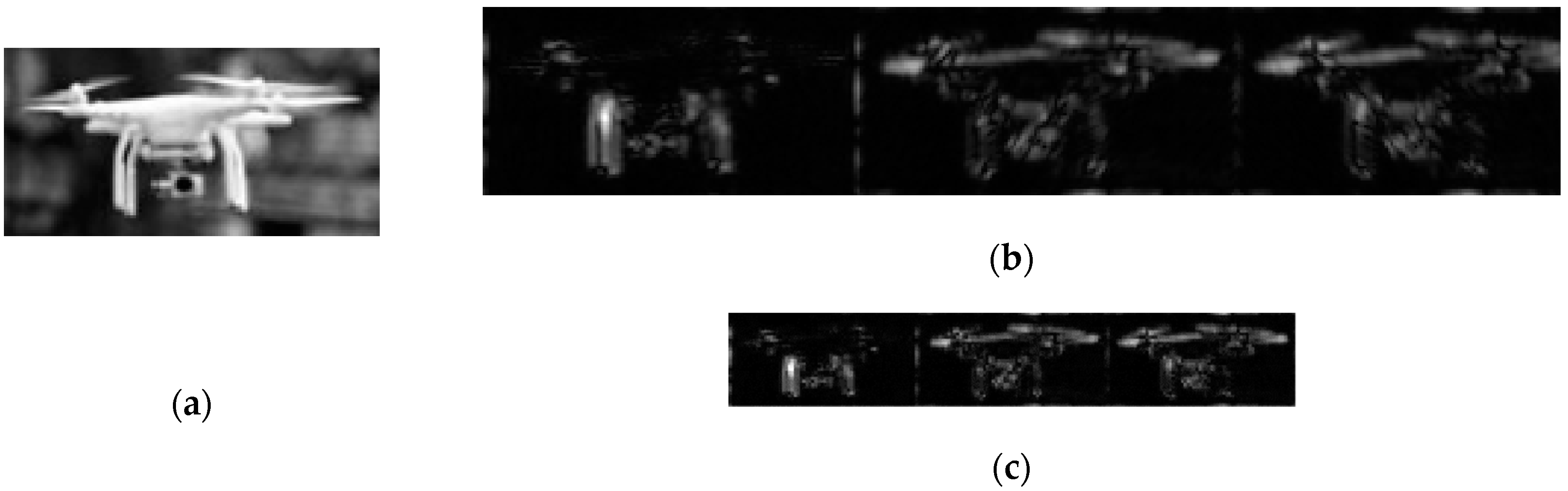
3.2. Preprocessing for Log-Gabor Feature Reduction by Downsampling

The sample image is transformed to 24,576-dimensional features by Log-Gabor filter with one scale and three orientations. Although the information of high-dimensional features is very rich, it is also redundant. NMFsc on such a high-dimensional matrix is not conducive to obtaining effective discriminative features. Also, the time of matrix decomposition of NMF is long, and it cannot achieve the best recognition performance. Therefore, we need a method to reduce the dimensions of Log-Gabor feature before NMFsc.

The method of downsampling is a simple and effective method. It has a fast speed and good recognition result according to the following experiments in this paper. It can reduce the original dimensions to 6144 or 1536 dimensions by using downsampling once or twice.

Figure 4a is an UAV image and Figure 4b is Log-Gabor filtering images of one scale and three orientations. Figure 4c is a downsampling image of Figure 4b. As shown in Figure 4, although the dimension of downsampling image is reduced, the main information is retained.

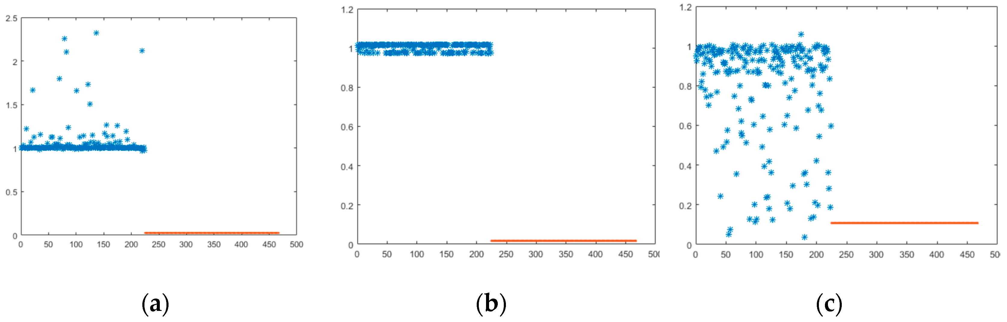
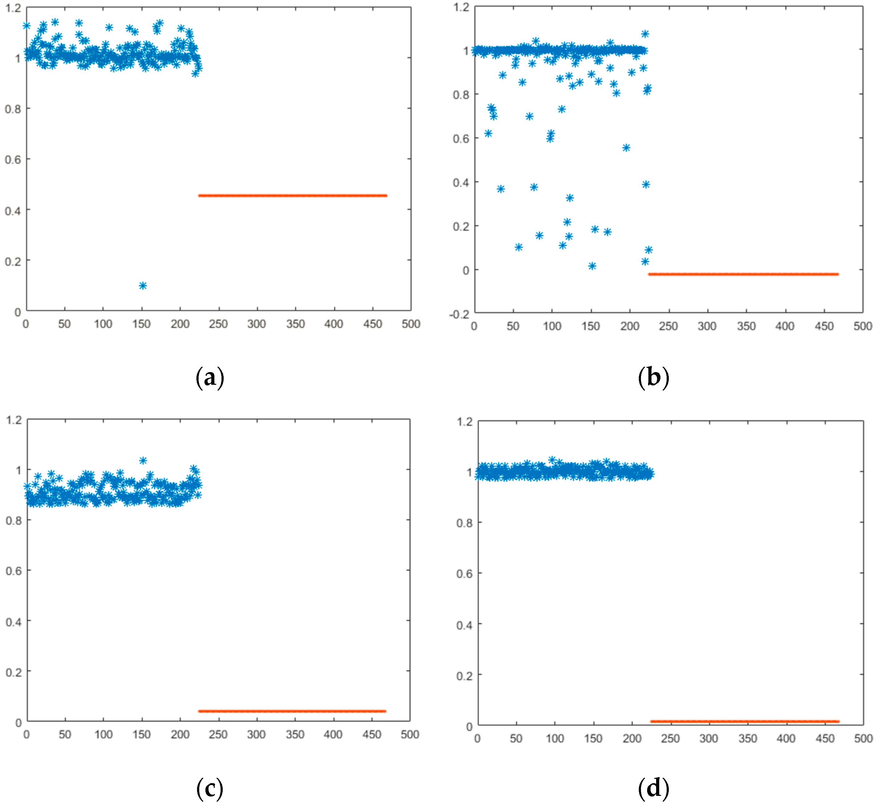
3.3. Feature Reduction by Non-Negative Matrix Factorization with Sparseness Constraints (NMFsc)

Lee and Seung published a non-negative matrix decomposition algorithm in Nature, which is a non-negative decomposition of all elements in a matrix in 1999. Negative results can be found in the results of matrix decomposition from the point of view of computation, but negative elements often lack physical meaning in practical problems. It has no negative values in the decomposition result because of its decomposition algorithm and has attracted the attention of many scientists and researchers.

Non-negative data are decomposed by non-negative data, and a simple and effective multiplicative iterative algorithm is used under non-negative constraints. The information about the local features of the object is contained in the learning base vector. Compared with the traditional principal component analysis (PCA), the results of the non-negative matrix factorization accord with the intuitive experience of the brain and have a clear physical meaning.

Non-negative matrix factorization (NMF) [23] is a method for finding such a representation. Given a non-negative data matrix V, NMF finds an approximate factorization V ≈ WH into non-negative factors W and H. The non-negativity constraints make the representation purely additive (allowing no subtractions), in contrast to many other linear representations such as principal component analysis (PCA) and independent component analysis (ICA).

Non-negative matrix factorization is a linear, non-negative approximate data representation. Denoting the (N-dimensional) measurement vectors v^t (t = 1, …, T), a linear approximation of the data is given by

$$v^t\approx {\displaystyle \sum _{i=1}^M{w}_i{h}_i^t=W{h}^t}$$

(3)

where W is an N × M matrix containing the basis vectors w_i as its columns.

Arranging the measurement vectors v^t into the columns of an N × T matrix V, V can now be described:

V ≈ WH

(4)

Given a data matrix V, the optimal choice of matrices W and H are defined to be those non-negative matrices that minimize the reconstruction error between V and WH. Various error functions have been proposed, perhaps the most widely used is the squared error (Euclidean distance) function.

$$E(W,H)={\Vert V-WH\Vert }^2={\displaystyle \sum _{i,j}{(V_{ij}-{(WH)}_{ij})}^2}$$

(5)

Although the minimization problem is convex in W and H separately, it is not convex in both simultaneously. Paatero gave a gradient algorithm for this optimization, whereas Lee and Seung devised a multiplicative algorithm that is somewhat simpler to implement and also showed good performance.

Definition NMF with sparseness constraints [24,25] (NMFsc) [12] as follows:

Given a non-negative data matrix V of size N × T, find the non-negative matrices W and H of sizes N × M and M × T (respectively) such that

$$E(W,H)={\Vert V-WH\Vert }^2$$

(6)

is minimized, under optional constraints

$$\begin{array}{l}\mathrm{sparseness}(w_i)=S_w,\forall i\\ \mathrm{sparseness}(h_i)=S_h,\forall i\end{array}$$

(7)

where w_i is the i:th column of W and h_i is the i:th row of H. Here, M denotes the number of components, and S_w and S_h are the desired sparsenesses of W and H (respectively). These three parameters are set by the user.

The process of feature reduction based on NMFsc:

(a)

Vectorization of the UAV sample image. The pixels of sample image are rearranged by column. The two-dimensional matrix A_i (i = 1, 2, …, m) of p × q is converted to n × 1 one-dimensional column vector v_i (where n = p × q). Then, m samples form n × m matrix V = [v₁ v₂ … v_m], of which each column of the matrix represents a sample image.

(b)

The formula V_n×m ≈ W_n×r H_r×m is written as v_i = Wh_i of column form, where the one column v_i of V corresponds to one column h_i of H. In other words, v_i is the linear combination of all row vectors of the base matrix W and the weight coefficient h_i. Therefore, under the W subspace, the h_i of low dimension can replace the original sample v_i of high dimension. When the NMF coefficient matrix of UAV image is solved, the image feature is obtained. The quality of projection coefficient h_i is determined by the base matrix W. The few base vectors of W should satisfy the description and approximation of raw data.

Figure 5 shows that information of image after downsampling of different number and NMFsc dimension reduction. As shown in Figure 5b,c, the information of image are reserved basically after downsampling once or twice. However, as the number of downsampling increasing, more and more information about image is lost. Hence, it is best to perform downsampling once or twice, whereby it reduces the dimensions while preserving the basic information of the image.

4. Target Recognition Using BP Neural Network

4.1. Principle of BP Neural Network

The BP algorithm is one of the most highly studied neural network (NN) algorithms due to its self-adaptation, self-learning, robustness, and generalizability. The BPNN with a three-layered topology can approach any nonlinear function with precision [26].

Equation (8) shows the relationship between the input and output of hidden neurons. The output of the whole network is y, the desired output is y’, and the error function is defined as e = y’ − y.

$$I_j=f_1(P_j)=f_1\left({\displaystyle \sum _{i=1}^n{w}_{ij}{X}_i+{\theta }_j}\right),(i=1,2,\cdots ,n;j=1,2,\cdots ,m),$$

(8)

$$y=f_2(Q)=f_2\left({\displaystyle \sum _{j=1}^m{w}_{jk}{I}_j+{\theta }_k}\right),(j=1,2,\cdots ,m;k=1)$$

(9)

The training process of BPNN continuously adjusts the weight and the threshold in order to minimize the network error. In this article, the transfer function for hidden layers is ‘tansig’ and that for the output layer is ‘purelin’.

Back propagation neural network (BPNN) is a simple architecture that involves a forward calculation of a network input vector to compare to a desired output vector and an error correction that propagates backwards from the output vector. The network consists of layers: an input layer, an output layer, and a usually hyperbolic tangent or sigmoid, to create a scaled output of the hidden processing element. All other processing elements in the hidden layer are summed and transformed in a similar manner. The output of the hidden layer becomes the input of the output layer, where summation and transformation also occur. During training, the output of output layer is compared to the desired output, and an error is computed. The weights are subsequently adjusted by taking the derivative of the error with respect to the connection weights. The procedure is repeated in an iterative fashion until a desired number of iterations are completed, or the error between the desired and calculated output is below a specified criterion.

4.2. The Design of the BP Neural Network Classifier

The design of the BP neural network classifier includes the design of the input layer, hidden layer, and output layer. It includes the design of the parameters of initial weight, neuron excitation function, learning rate, expectation error, and more. The steps to build the BP neural network are as follows:

(1)

Designing the input layer: the input node equals the extracted feature dimension of image. The actual input node is the reduction feature dimension by NMFsc in this paper.

(2)

Designing the hidden layer:

(a)

The number of hidden layers—increasing the number of hidden layers can improve the generalization performance of the network, reduce the error, and increase the recognition rate, but also make the network complex and the training time long. Hence, three layers of neural network are used in this paper.

(b)

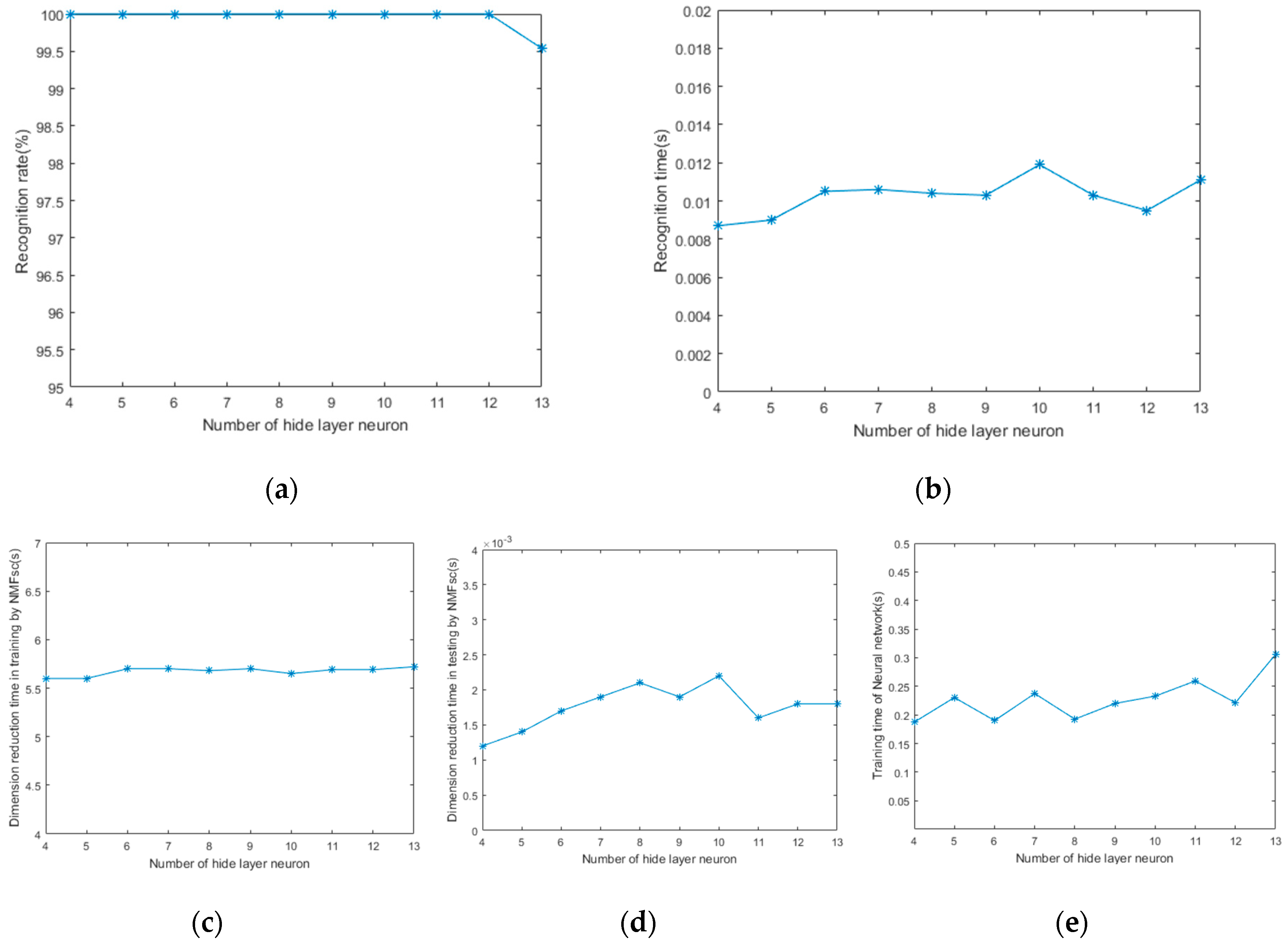
The number of hidden layer neurons—the number of the hidden layer neurons should be in a reasonable range. Too few and it will be easy to fall into the local minimum and the trained network may not converge, with low recognition rate and poor fault tolerance. Too many will make the network structure complex, generalization ability poor, training time long, real-time performance bad, and recognition rate low. The recommended empirical formulas are provided for reference in practice:

$$n_1=\sqrt{n+m}+a$$

(10)

$$n_2=\sqrt{n\times m}$$

(11)

The number of neurons in the hidden layer is obtained from formulas, in which m is the number of neurons in the output layer, n is the number of neurons in the input layer, and a is the integer of 1–10.

It is easier to observe and control the accuracy by adjusting the number of hidden layer neurons than increasing the number of hidden layers. Therefore, in general, the number of neurons in the hidden layer is considered for change first. When the single hidden layer cannot meet the requirements, other hidden layers will be added. However, it is best to have no more than two hidden layers. It has been proven, theoretically, that the three-layer BP neural network with sigmoid nonlinear function is able to approximate any continuous function to any accuracy.

(3)

Designing output layer—the categories of identifying target are directly used for the output node of the neural network. In this paper, as only the UAV target needs to be identified, the number of output nodes is set to 1.

(4)

Initialization of weight and threshold with uniformly distributed random numbers—it is very important for the initialization of weight and threshold in nonlinear systems. If the initial weight is too large, the weighted input will be entered into the saturation area of the activation function, which leads to the stagnation of the adjustment. Randomization is particularly important in the implementation of the BP model. If the weights are not initialized randomly, the learning process may not converge. In this paper, the initial weights are taken from the random numbers between (−1,1).

(5)

Giving the input samples, desired output, neuron activation function, and learning rate—the activation function has a considerable influence on the convergence effect of the network. Each input of the neuron corresponds to a specific weight, and the weighted sum of the input determines the activation state of the neuron. The learning rate determines the variation of the weight during each training. Too high a learning rate leads to network oscillation, and too low a learning rate leads to slow convergence and long training times. In general, it tends to choose a smaller learning rate to ensure the stability of the system. In this paper, expected error is set to 0.01, the transfer function of the hidden layer neuron is a tangent S function ‘tansig’, the transfer function of the output layer is a linear function ‘purelin’, the training function is ‘LM’, and the number of learning times is set to 10,000.

(6)

Training the sample data—with the sample data inputted, the actual output of the hidden layer and output layer are obtained, and the hidden layer error and the output layer error are calculated. If the error cannot reach the set value, the error signal is returned along the original path, and the network weight and threshold are corrected according to the error feedback. When the error or the learning time reach the set value through repeating the above process, the training is completed.

5. Experiments Results

To evaluate our proposed method, we collect 2000 UAV images from internet and our practical shooting videos, which 1000 images for train and 1000 images for test. All calculations are implemented using MATLAB 2015b on an Intel i5 2.6 GHz processor with 8 GB memory and Windows 10 64-bit operating system.

By counting the aspect ratio of the UAV images, the aspect ratio 1:2 is obtained, and the all sample images are normalized to 64 × 28 size.

(1) Candidate region extraction

Figure 6 shows the candidate regions with different degree using the EdgeBoxes extraction method. The parameter is optimized for detecting boxes at intersection over union (IoU) of 0.7. The other parameters are set alpha = 0.65, beta = 0.90, opts.multiscale = 0, model.opts.sharpen = 0. The number of candidate regions in Figure 6a is more than the number in Figure 6b with the parameter max number of boxes. However, a large amount of candidate regions increases the calculation work, which will lead to inefficiency. Hence, we use an appropriate parameter, such as Figure 6c. For the image size 500 × 281, the time is 0.068 s. The time difference is about 0.001 s with the parameter “max number of boxes” varying from 50 to 1000.

(2) Feature extraction and dimensionality reduction:

Log-Gabor feature is extracted from candidate regions of the steps above. In order to speed up the detection, Log-Gabor filters of one scale and three directions are adopted. The filter time of Log-Gabor for the single sample image is 0.003 s, which fully satisfies the real-time need. These amplitudes of Log-Gabor filtering image are used in this paper, and all column pixels are concatenated into a single vector. It generates 24,576-dimensional feature vector.

Although the 24,576 high-dimensional feature information is rich but also redundant. NMF on such a high-dimensional matrix is not beneficial to getting effective identification feature, and the matrix decomposition time is long. Also, it cannot achieve the best recognition rate. The method of downsampling is a simple and easy method, which has a fast speed and good recognition result. The dimension of the feature is reduced to 6144~12 dimensions by downsampling. In order to test the effect of downsampling and NMFsc on the recognition results, the normalized 224 positive sample images and 243 negative sample images are used. The feature is reduced to 10 dimensions by NMFsc, which is used as the input of the neural network. The number of hidden layers are four, and the neural network has three layers. The experimental results are shown in the

Table 2. Experimental results of Log-Gabor feature downsampling and NMFsc.

Feature Dimensions of Log-Gabor	Number of Downsampling	Dimension Reduction Time by NMFsc in Training (s)	Recognition Rate (%)	Error Rate (%)
24,576	0	97	91	0
6144	1	22	100	0
1536	2	5.6	100	0
384	3	1.5	100	0
96	4	0.4	99.5	0
24	5	0.09	94	0
24	6	Not using NMFsc	91	0
12	6.5	Not using NMFsc	85	0
6	7	Not using NMFsc	48	0

.

As shown in Table 2, using the original 24,576-dimensional Log-Gabor features are not conducive to matrix transformation of NMFsc and improving the recognition rate. Although the 24,576-dimensional features have abundant information, they are redundant. High-dimensional feature makes the NMFsc complex, and leads to long computing times. Also, it is difficult to effectively extract discriminative information. The recognition rate using the original 24,576-dimensional Log-Gabor features is not as good as the downsampling.

The dimensionality reduction time of NMFsc decreases with the feature dimension. The recognition performance remains basically unchanged when the Log-Gabor feature dimensions are above 384. With the feature dimensions decreasing, the recognition performance begins to decline, which indicates that the discrimination information is lost in the case of downsampling.

Figure 7 shows the probability distribution of recognition result for the normalized 224 positive samples and 243 negative sample images. The ordinate (Y-axis) of Figure 7 is the probability distribution of recognition rate, and the abscissa (X-axis) is 467 sample images. The 224 positive samples are from 1 to 224 on abscissa, and 243 negative samples are from 244 to 467. For positive samples, the performance is best when the probability is greater than or equal to 1 and, for negative samples, the performance is best when the probability is close to 0.

As shown in Figure 7, the results of 6144- and 1536-dimensional Log-Gabor features are very similar. The result of 6144 dimensions is slightly better than of 1536 dimensions, while the results of 12-dimensional Log-Gabor features without using NMFsc reduction is very different from others, which it has poor performance. It is hard to distinguish between positive samples and negative samples from Figure 7c. The results show that the feature reduced by NMFsc contains the main discriminating information.

Table 3. Experimental comparison of NMFsc and NMF.

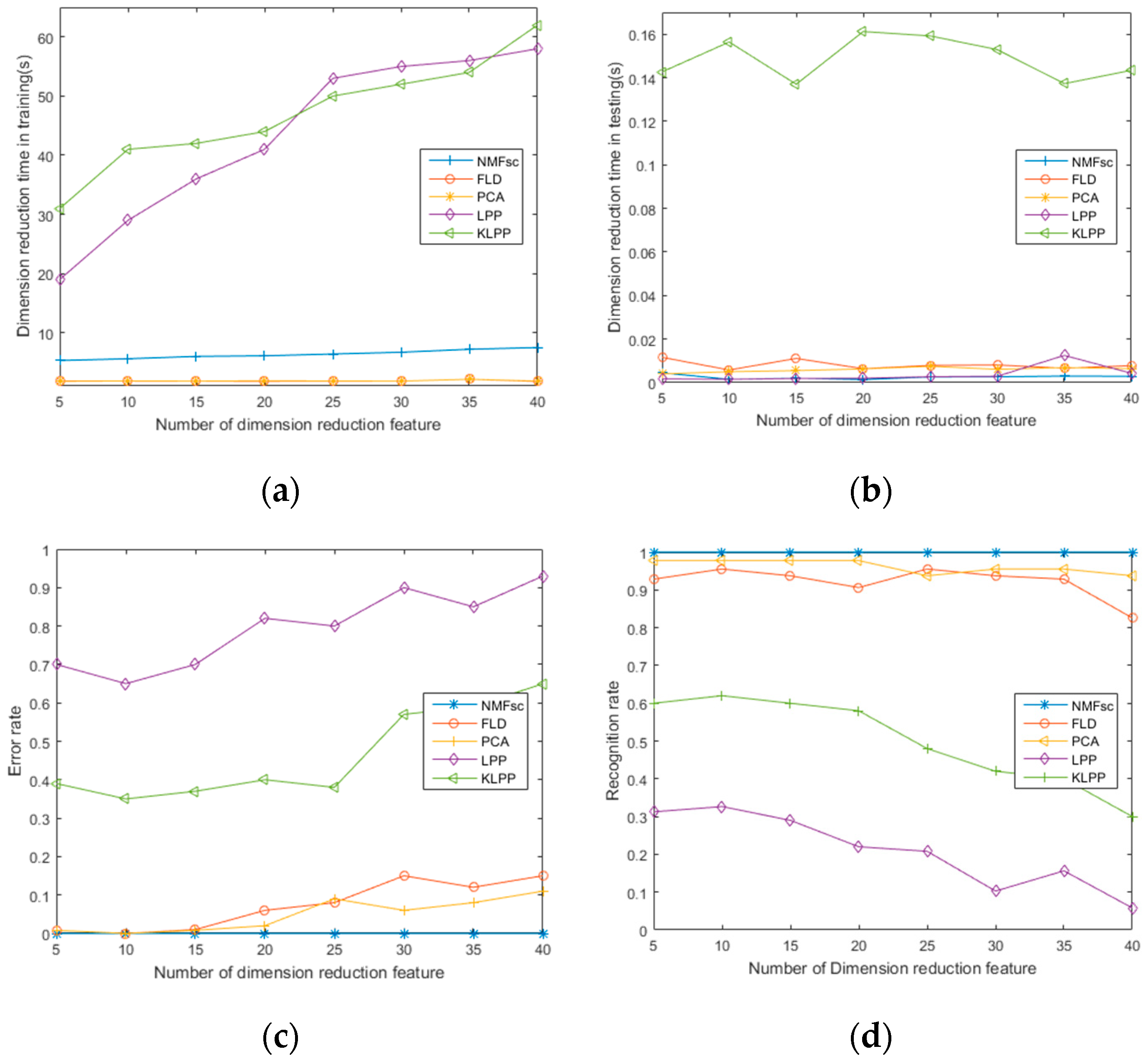
	Recognition Rate (%)	Error Rate (%)	Average Dimension Reduction Time in Training (s)	Average NN Training Time (s)	Average Dimension Reduction Time in Testing (s)	Average Recognition Time (s)
NMFsc	100	0	5	0.2416	0.0021	0.0105
NMF	0.9967	0	15	0.2459	0.0026	0.0121

shows the comparable results of the classical NMF and NMF with sparseness constraint (NMFsc). We can see that the NMFsc is better than the classical NMF in the dimension reduction time and the recognition rate.

After downsampling twice of the original Log-Gabor feature, the 1536-dimensional features are formed, and then the 1536-dimensional features are reduced to 5~40 dimensions by different dimension reduction method. The better dimension reduction algorithm is selected by comparing the comprehensive effect of dimension reduction and recognition result. The probability distribution of the simulation results is shown in Figure 8, and the dimensionality reduction time of each method is shown in

Table 4. Dimension reduction time of different methods.

Method	Average Time for Training Sample (s)	Average Time for Testing Sample (s)
PCA	1.87	0.006
FLD	1.88	0.021
NMFsc	5.6	0.002
LPP	43	0.004
KLPP	48	0.153

.

PCA and Fisher linear discriminant (FLD) analysis are simple calculations, highly efficient and having the shortest time in dimension reduction than others. NMF can be considered to be an optimization problem, which a simple iterative method for solving U and V matrixes. The solving method has fast convergence speed and small storage space. The dimension reduction time of the manifold learning algorithm, LPP, is longer because the dense matrix is to be solved. The dimension reduction time of KLPP algorithm is also longer because the data are mapped to kernel space.

Figure 9 shows the experimental comparison of different reduction method. As shown in Figure 9, the dimension reduction time increases with the increasing of the feature dimension, and the difference of various methods is large. The recognition rate reaches the best when feature dimension is 10 to 20.

By analyzing, comprehensively, dimension reduction efficiency, training performance, and recognition results, NMFsc obtains the coordination in real-time, accuracy, network performance, and other aspects. The combination of NMFsc and BP neural network can achieve better recognition results. When the dimension is in the range of 5–15, the recognition rate is better. When the dimension exceeds 20, the recognition rate begins to decrease, and training and recognition time increase slowly. Considering real-time and accuracy, 10-dimensional Log-Gabor features are selected for subsequent training and recognition.

(3) Training and recognition of BP neural network

Both the number of hidden layers and the number of hidden layer neurons have an effect on the accuracy and time of recognition for BP neural network. According to Formula (10), the number of neurons of hidden layer ranges from 4 to 13 when using a three-layer network. Precision is set to 0.01. As shown in Figure 10, the performance of training and recognition varies with the number of neurons in the hidden layer. As the number of hidden layer neurons increases, the training time slowly increases. The recognition rate is 100% when the number of neurons is from 4 to 12. While the number of neurons continues to rise, the recognition rate begins to decrease. The result shows that regarding the number of neurons in the hidden layer, more is not necessarily better, and there will be an extreme value. The best number of neurons can be selected to achieve the best recognition performance through many experiments.

We select 1000 images for UAV detection test from the frame of our practical shooting videos. Figure 11 shows the UAV detection results. There are 993 UAV images that are accurately detected, and 5 UAV objects that are not detected because of their complicated background, poor illumination, and far distance. The accuracy rate is 99.7%. Also, there are 16 candidate regions of error recognition. This is because of the similarity between the UAV and candidate regions in the case of certain illumination, shape, and angle.

(4) Experimental comparison with FasterR-CNN

Deep learning has achieved great success in the application of large samples. However, for the small sample of UAV images, how about the performance? We have done some experiments to address this. Faster R-CNN [27] is used in the experiment, and VGG-16 is selected for the feature extraction network. A total of 300 UAV images are selected as training samples to be sent to the network. The experimental result is shown in Figure 12. The AP (Average Precision) value is 0.984.

A comparison between Faster R-CNN and our method is shown in

Table 5. Comparison with Faster-RCNN.

	Precision (%)	Average Testing Time (s)	Average Training Time	Computer Cost	Image Annotation
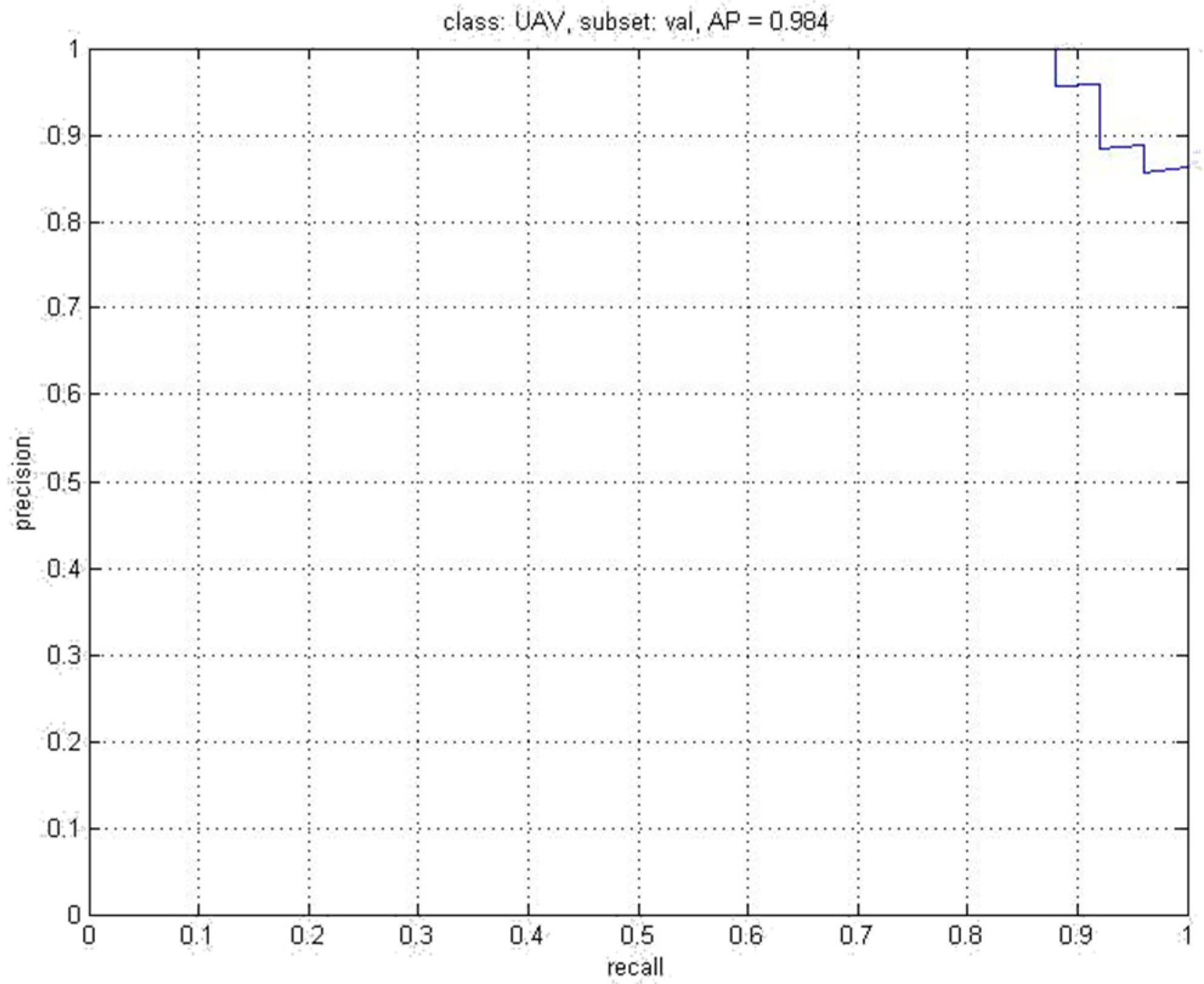
Faster R-CNN [27]	98.4	0.12	14 h	High	Many
Our method	98.6	0.16	seconds	Low	Less

. The precision of the two methods is very close. However, regarding the training time, computer cost, and image annotation, our method has the advantage. Experimental results show that Faster R-CNN takes 14 h of training time cost, while our method only requires 6 s for training. Deep learning has high hardware requirements. Our method does not require a large number of samples to be trained and has small time cost, good real-time performance, and high precision. By the comprehensive analysis, the method proposed in this paper is feasible.

6. Conclusions

For the problem that the BP neural network is hard to effectively train to discriminate high-dimensional features, NMFsc feature reduction and the BP neural network are used together in this paper. The high-dimensional Log-Gabor features are reduced to low dimensions by the NMF with sparseness constraint algorithm, and then input into the BP network to train the classifier to improve the recognition performance. The experimental results show that the method overcomes the problem of both working in real-time and the accuracy of the traditional dimensionality reduction method, and the feature reduction is superior to the common methods, such as PCA, FLD, LPP, KLPP, and others. It is especially suitable for the target recognition of high-dimension features. For the UAV object recognition and detection in this paper, we achieve satisfactory results. How to reduce error recognition will be the question to address by follow-up research work—the methods of moving object detection could be used. Also, deep learning techniques for small samples would be researched in this field.

References

- Jian, C.F.; Li, M.; Qiu, K.Y.; Zhang, M.Y. An improved NBA-based step design intention feature recognition. Future Gener. Comput. Syst. Int. J. Escienc. 2018, 88, 357–362. [Google Scholar] [CrossRef]
- Zhao, Y.X.; Zhou, D.; Yan, H.L. An improved retrieval method of atmospheric parameter profiles based on the BP neural network. Atmos. Res. 2018, 213, 389–397. [Google Scholar] [CrossRef]
- Qiao, J.F.; Li, M.; Liu, J. A fast pruning algorithm for neural network. Acta Electron. Sinca 2010, 38, 830–834. [Google Scholar]
- Sheng, Y.X. Drivers’ state recognition and behavior analysis based on BP neural network algorithm. J. Yanshan Univ. 2016, 40, 367–371. [Google Scholar]
- Zhao, R.; Qi, C.J.; Duan, L.F. Identification of rice rolling leaf based on BP neural network. J. South. Agric. 2018, 49, 2103–2109. [Google Scholar]
- Liu, Y.G.; Hou, L.L.; Qin, D.T.; Hu, M.H. Coal Seam Hardness Hierarchical Identification Method Based on BP Neural Network. J. Northeast. Univ. (Natl. Sci.) 2018, 39, 1163–1168. [Google Scholar]
- Gan, L.; Tian, L.H.; Li, C. Traffic sign recognition method based on multi-feature combination and BP neural network. Comput. Eng. Des. 2017, 38, 2783–2813. [Google Scholar]
- Ma, Y.; Lv, Q.B.; Liu, Y.Y. Image sparsity evaluation based on principle component analysis. Acta Phys. Sin. 2013, 62, 1–11. [Google Scholar]
- Zhang, L.M.; Qiao, L.S.; Chen, S.C. Graph-optimized locality preserving projections. Pattern Recognit. 2010, 43, 1993–2002. [Google Scholar] [CrossRef]
- Raghavendra, U.; Rajendra Acharya, U.; Ng, E.Y.K.; Tan, J.H.; Gudigar, A. An integrated index for breast cancer identification using histogram of oriented gradient and kernel locality preserving projection features extracted from thermograms. Quant. InfraRed Thermogr. J. 2016, 13, 195–209. [Google Scholar] [CrossRef]
- Cui, Z.Y.; Cao, Z.J.; Yang, J.Y.; Feng, J.L.; Ren, H.L. Target recognition in synthetic aperture radar images via non-negative matrix factorisation. IET Radar Sonar Navig. 2015, 9, 1376–1385. [Google Scholar] [CrossRef]
- Hoyer, P.O. Non-negative matrix factorization with sparseness constraints. J. Mach. Learn. Res. 2004, 5, 1457–1469. [Google Scholar]
- Uijlings, J.; van de Sande, K.; Gevers, T.; Smeulders, A. Selective search for object recognition. Int. J. Comp. Vis. 2013, 104, 154–171. [Google Scholar] [CrossRef]
- Girshick, R.; Donahue, J.; Darrell, T.; Malik, J. Rich feature hierarchies for accurate object detection and semantic segmentation. arXiv, 2014; arXiv:1311.2524. [Google Scholar]
- Girshick, R. Fast R-CNN. arXiv, 2015; arXiv:1504.08083. [Google Scholar]
- Carreira, J.; Sminchisescu, C. CPMC: Automatic object segmentation using constrained parametric min-cuts. IEEE Trans. Pattern Anal. Mach. Intell. 2012, 34, 1312–1328. [Google Scholar] [CrossRef] [PubMed]
- Endres, I.; Hoiem, D. Category-independent object proposals with diverse ranking. IEEE Trans. Pattern Anal. Mach. Intell. 2014, 36, 222–234. [Google Scholar] [CrossRef]
- Alexe, B.; Deselaers, T.; Ferrari, V. Measuring the objectness of image windows. IEEE Trans. Pattern Anal. Mach. Intell. 2012, 34, 2189–2202. [Google Scholar] [CrossRef] [PubMed]
- Rahtu, E.; Kannala, J.; Blaschko, M. Learning a category independent object detection cascade. In Proceedings of the 2011 IEEE International Conference on Computer Vision (ICCV), Barcelona, Spain, 6–13 November 2011; pp. 1052–1059. [Google Scholar]
- Zitnick, C.L.; Dollár, P. Edge boxes: Locating object proposals from edges. Lecture Notes in Computer Science. In Computer Vision–ECCV; Springer: Cham, Switzerland, 2014; pp. 391–405. [Google Scholar]
- Cheng, M.M.; Zhang, Z.; Lin, W.Y.; Torr, P. BING: Binarized normed gradients for objectness estimation at 300 fps. In Proceedings of the IEEE Conference on Computer Vision and Pattern Recognition, Columbus, OH, USA, 23–28 June 2014; pp. 3286–3293. [Google Scholar]
- Rantalankila, P.; Kannala, J.; Rahtu, E. Generating object segmentation proposals using global and local search. In Proceedings of the 2014 IEEE Conference on Computer Vision and Pattern Recognition (CVPR), Columbus, OH, USA, 23–28 June 2014; pp. 2417–2424. [Google Scholar]
- Lee, D.D.; Seung, H.S. Learning the parts of objects by non-negative matrix factorization. Nature 1999, 401, 788–791. [Google Scholar] [CrossRef] [PubMed]
- Jiao, Y.; Zhang, Y.; Chen, X.; Yin, E.; Jin, J.; Wang, X.Y.; Cichocki, A. Sparse group representation model for motor imagery EEG classification. IEEE J. Biomed. Health Inform. 2018. [Google Scholar] [CrossRef] [PubMed]
- Zhang, Y.; Nam, C.S.; Zhou, G.X.; Jin, J.; Wang, X.Y.; Cichocki, A. Temporally constrained sparse group spatial patterns for motor imagery BCI. IEEE Trans. Cybern. 2018, 1–11. [Google Scholar] [CrossRef]
- Ding, S.F.; Su, C.Y.; Yu, J.Z. An optimizing BP neural network algorithm based on genetic algorithm. Artif. Intell. Rev. 2011, 36, 153–162. [Google Scholar] [CrossRef]
- Ren, S.; He, K.; Girshick, R.; Sun, J. Faster R-CNN: Towards real-time object detection with region proposal networks. IEEE Trans. Pattern Anal. Mach. Intell. 2015, 39. [Google Scholar] [CrossRef] [PubMed]