A Feature Selection and Classification Method for Activity Recognition Based on an Inertial Sensing Unit

Abstract

The purpose of activity recognition is to identify activities through a series of observations of the experimenter’s behavior and the environmental conditions. In this study, through feature selection algorithms, we researched the effects of a large number of features on human activity recognition (HAR) assisted by an inertial measurement unit (IMU), and applied them to smartphones of the future. In the research process, we considered 585 features (calculated from tri-axial accelerometer and tri-axial gyroscope data). We comprehensively analyzed the features of signals and classification methods. Three feature selection algorithms were considered, and the combination effect between the features was used to select a feature set with a significant effect on the classification of the activity, which reduced the complexity of the classifier and improved the classification accuracy. We used five classification methods (support vector machine [SVM], decision tree, linear regression, Gaussian process, and threshold selection) to verify the classification accuracy. The activity recognition method we proposed could recognize six basic activities (BAs) (standing, going upstairs, going downstairs, walking, lying, and sitting) and postural transitions (PTs) (stand-to-sit, sit-to-stand, stand-to-lie, lie-to-stand, sit-to-lie, and lie-to-sit), with an average accuracy of 96.4%.

1. Introduction

With the rapid development of artificial intelligence, activity recognition has become an important emerging field of research. Different technical means that recognize the human activities of users employing different embedded sensors have been actively studied [1]. Early research focused on recognizing activities with signals coming from one or more standalone motion sensors that were attached to the human body, at locations chosen by the researcher. Because vision-based activity recognition analyses include a high cost and environmental restrictions [2], human activity recognition (HAR) systems have been used to receive the state of the user by wearable inertial sensors attached to the user’s body to measure and evaluate their action patterns [3,4].

Raw data collected from sensors recognize human activities through machine learning algorithms [5,6]. The main application areas of this research are low-complexity systems such as single-chip microcomputers, which only use a small amount of data. Accurate signal processing and feature selection are fast becoming key problems in the field of attitude recognition.

Most wearable devices with sensors are still limited by hardware resources, preventing real-time and fast access to activity recognition results that require a lot of computation [7]. Therefore, in order to make HAR more applicable to wearable devices with limited hardware resources, traditional analysis methods based on deep learning theory have mostly been abandoned by researchers [8].

The feature extraction methods of the HAR system can be divided into three categories, namely, time features, frequency features, and a combination of both [9]. Jarraya et al. selected 280 features from a total of 561 by means of a nonlinear Choquet integral feature selection approach, classified six basic actions by using the random forest, and finally obtained a better classification effect. However, the large number of selected features affected the performance of the classifier [10]. Doewes et al. used the minimum redundancy and maximum correlation feature selection algorithms to analyze the number of selected features and the classification accuracy under different proportions of training sets and test sets, and considered the operation time of the classification process. However, only two classifiers, the support vector machine (SVM) and multilayer perception (MLP), were analyzed, and the MLP training easily dropped into a local optimum, which resulted in a training failure and an affected accuracy evaluation [11]. Li et al. proposed a feature set selection algorithm based on adaptive character activity and improved genetic algorithm, which could dynamically guide the process of feature selection and obtain small-scale feature sets on the basis of a higher classification accuracy and a faster running time. However, the proposed algorithm could not deal with a large search space, including a large feature space and a large-scale mode [12]. Ridok et al. proposed a feature selection method based on a fast correlation-based filter (FCBF) to achieve data preprocessing, and proved that the accuracy of classification could reach 100%. However, only the Artificial Immune Recognition System 2 (AIRS2) algorithm was used as the classification model, which could not determine if it was applicable to other classifiers [13].

On the basis of fully studying the time-domain and frequency-domain features of acceleration and angular velocity, this study used the feature selection method to find the optimal feature subset, and further employed a variety of classification models to evaluate the classification accuracy. The selection of classifiers for activity recognition was determined by many factors. In addition to accuracy, factors such as ease of development, computational complexity, and speed of execution could also affect the choice of classifiers [14]. Although the deep learning algorithm could achieve a high accuracy, the paper applied a low complexity system with a small amount of data, and the classifier structure was more complicated and had higher hardware requirements. Feature selection is the process of selecting a subset of original features based on clearly defined evaluation criteria, which can eliminate irrelevant and redundant features [15]. Feature selection does not change the original representation of the feature set, compared to other dimensionality reduction techniques based on projection, such as linear discriminate analysis or principal component analysis [16], and online classification with the selected features is more flexible. The organization of this article is as follows: In the second section, the system framework is introduced; in the third section, the signal processing and feature selection method based on SVM are introduced; in the fourth section, the classification effects of the feature sets are verified by multiple classification models, and the experimental results are analyzed and discussed; and the fifth section presents the conclusions of this research.

2. System Frameworks

The HAR model proposed in this paper is composed of six parts—signal acquisition, signal processing, feature extraction, feature selection, classification model training, and classification prediction (as shown in Figure 1). In this study, the data were obtained from a tri-axial acceleration sensor and a tri-axial angular velocity sensor for signal processing, feature calculation, and feature selection. Finally, the selected features were trained for classification and prediction [17].

A total of 50% of the data was used for feature selection, 35% of the data was used for classification model training, and the other 15% was used for precision evaluation [18]. Signal acquisition is the collection and processing of sensor data from available sources. In general, signal conditioning (e.g., noise reduction, digitization amplification) is always required to adapt the sensing signal to the application requirements [19]. The feature extraction process is responsible for obtaining meaningful features that describe the data, and allows for a better representation and understanding of the phenomena under study. The extracted features provide the most effective features through feature selection and input them into the classifier in order to train the classification model [20]. Finally, the classification model is verified.

3. Signal Processing, Feature Extraction, and Feature Selection

3.1. Signal Processing and Feature Extraction

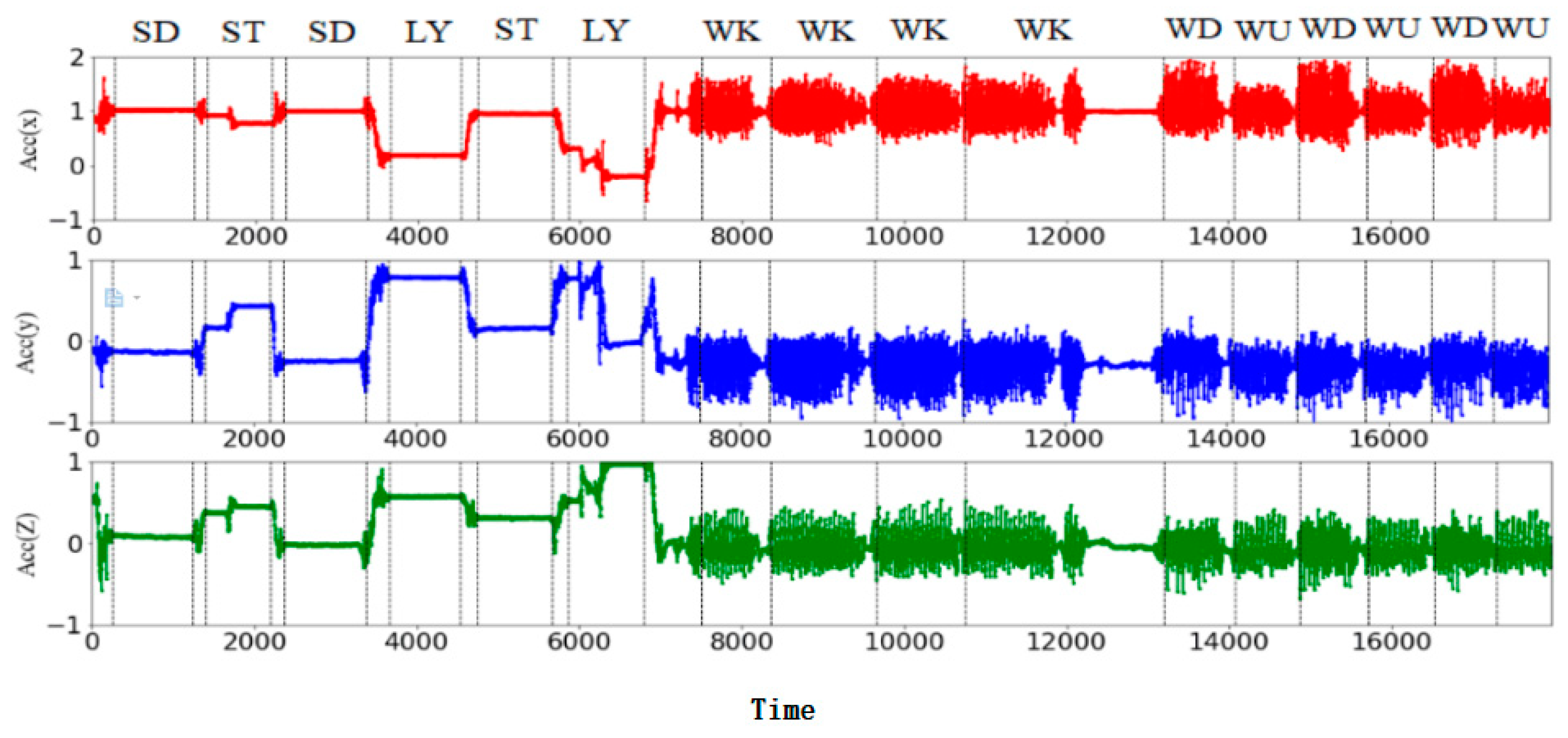
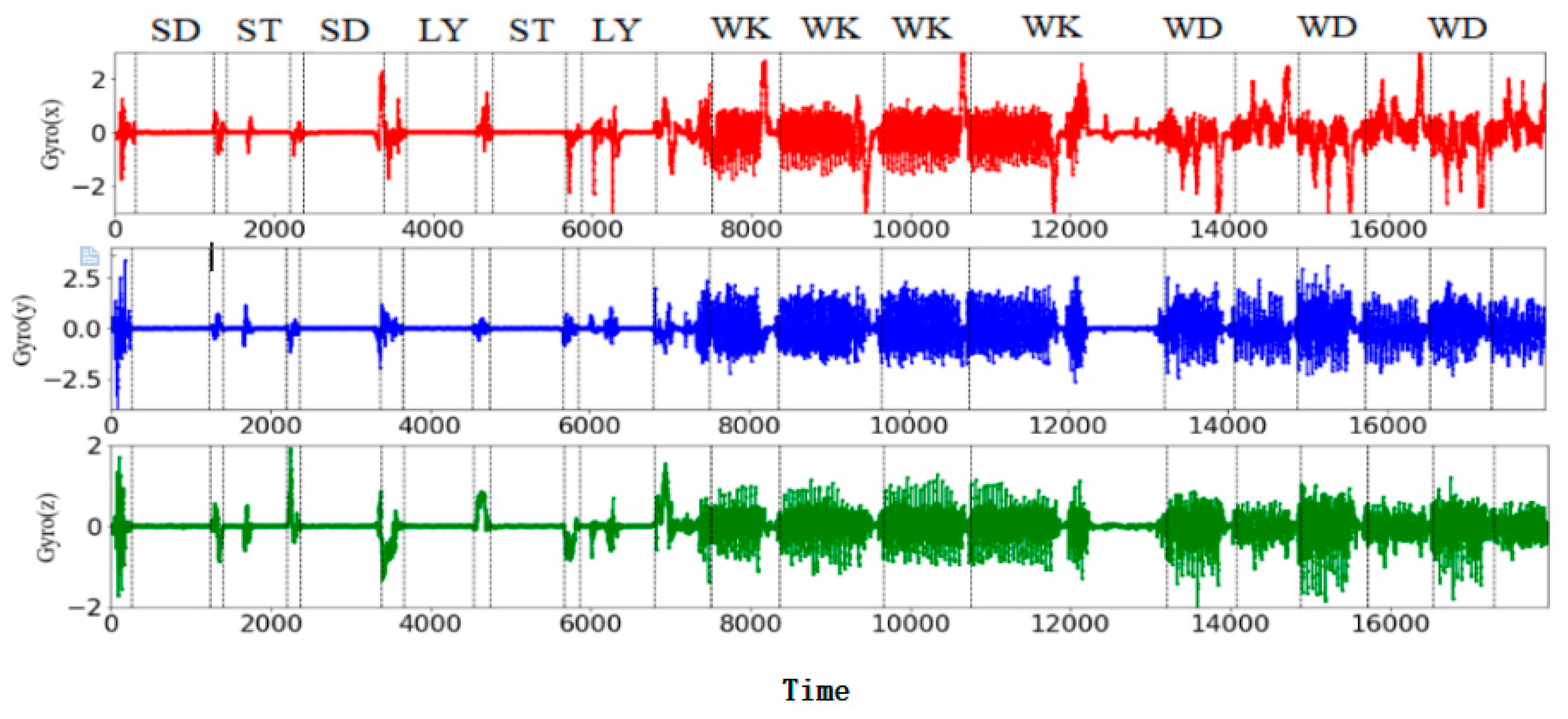
Firstly, the tri-axial acceleration signal and tri-axial angular velocity signal of the inertial sensor corresponding to six basic motions (walking (WK), walking upstairs (WU), walking downstairs (WD), standing (SD), sitting (ST), and lying (LY)) were obtained in the experiment, as shown in Figure 2 and Figure 3.

Since the energy spectrum of human body motion is mainly in the range of 0–15 Hz, a median filter and a third-order low-pass Butterworth filter with a 20-Hz cutoff frequency were used to filter the six-axis signal to remove noise. The angular velocity signal was high-pass filtered to remove any DC offset that would affect the gyroscope. Similarly, a low-pass Butterworth filter with a cut-off frequency of 0.3 Hz was used to separate gravity acceleration signals from tri-axial acceleration signals, including tAcc-xyz, tGyro-xyz, and tGravityacc-xyz [21]. The resulting acceleration signals, gravity acceleration signals, and angular velocity signals provide information about the user’s body movements, the person’s orientation (for example, helping to distinguish between lying down and standing up), and the movement patterns in which people perform certain activities [22].

Subsequently, the body acceleration signals and angular velocity signals were calculated with the difference calculation to obtain Jerk signals (a certain amount of information was known about the characteristics of related activities, and was successfully applied to the test of patients [23]), respectively represented by taccjerk-xyz and tgyrojerk-xyz.

In addition, the formula $\sqrt{x^2+y^2+z^2}$ was used to calculate the triaxial acceleration, triaxial angular velocity, and gravity component, that is, tAccMag, tGyroMag, and tGravityAccMag, respectively [24]. The processed signal allowed the reduction of data dimensions and meant that the data were independent of the direction.

Furthermore, it was necessary to solve the angle between the tri-axial signal vector and the gravity component, that is, tAccAng and tGyroAng, respectively. The angle between the earth’s gravity and the sensor device had a good effect on the static action.

Finally, the real value Fast Fourier Transformation (FFT) algorithm was used to transform these windows into the frequency domain, resulting in facc-xyz, fgyro-xyz, and faccjerk-xyz [25].

The commonly used features are statistical measures including the mean, variance, standard deviation, root mean square [26], fast Fourier transform (FFT), coefficients [27], and discrete cosine transform (DCT) coefficients [28].

After the signal processing was completed as described above, these signals were used as variables for estimating the feature vector of each mode, and the behavior was modeled using a windowed method (the average human walking rhythm is at least 1.5 steps/second); each window sample preferably had at least a complete walking cycle. The rectangular sensor window of the overlapping window factory was used to extract the acceleration sensor signal. After selecting the appropriate window factory, various features were extracted from the acceleration signal of the single window factory to obtain the feature vector.

Table 1. Time domain features of the x-axis.

Type Description	Definitions
Arithmetic mean tAcc-X	$\overline{v}=\frac{1}{N}{\displaystyle \sum _{i=1}^N{v}_i}$
Sample Standard deviation tAcc-X	$s={\left(\frac{1}{N-1}{\displaystyle \sum _{i=1}^N{(v_i-\overline{v})}^2}\right)}^{1/2}$
Sample Variance tAcc-X	$s^2=\frac{1}{N-1}{\displaystyle \sum _{i=1}^N{(v_i-\overline{v})}^2}$
Median tAcc-X	$median\left(v_i\right)$
Median absolute deviation tAcc-X	$median\left(\left|v_i-median\left(v_i\right)\right|\right)$
Largest values tAcc-X	$\max \left(v_i\right)$
Smallest value tAcc-X	$\min \left(v_i\right)$
Sample Range tAcc-X	$r=\max \left(v_i\right)-\min \left(v_i\right)$
Inter-quartile range tAcc-X	$IQR=Q3\left(v_i\right)-Q1\left(v_i\right)$
Mean crossing rate tAcc-X	$\frac{1}{N-1}{\displaystyle {\sum }_{i=1}^{N-1}{\displaystyle \prod \{\left(v_i-\overline{v}\right)\ast \left(v_{i-1}-\overline{v}\right)<0\}}}$
Skewness tAcc-X	$skew=\frac{{\displaystyle \sum {\left(V-\mu \right)}^3}}{N{\sigma }^3}$
Kurtosis tAcc-X	$Kurt=\frac{{\displaystyle \sum {\left(V-\mu \right)}^3}}{N{\sigma }^4}-3$
Curve Length tAcc-X	$CL=\frac{1}{N-1}{\displaystyle {\sum }_{i=2}^N\left|v_{i-1}-v_i\right|}$
Slope tAcc-X	$Slop=\max \left|v_{i-1}-v_i\right|$
Power tAcc-X	$P\left(v\right)=\frac{1}{N}{\displaystyle {\sum }_{i=1}^N{\left(v_i\right)}^2}$
Root Mean Square tAcc-X	$RMS={\left(\frac{1}{N}{\displaystyle {\sum }_{i=1}^N{v}_i^2}\right)}^{1/2}$
Mean Euclidean distance tAcc-X	$L2=\frac{1}{N-1}\sqrt{{\displaystyle {\sum }_{i=2}^N{\left(v_{i-1}-v_i\right)}^2}}$
10th percentile tAcc-X	$percentile\left(v,10\right)$
25th Percentile tAcc-X	$percentile\left(v,25\right)$
50th Percentile tAcc-X	$percentile\left(v,50\right)$
75th Percentile tAcc-X	$percentile\left(v,75\right)$
90th Percentile tAcc-X	$percentile\left(v,90\right)$

shows 22 measures applied to the x-axis.

Table 2. Correlation feature between signal pairs of the x-axis and y-axis.

Type Description	Definitions
Covariance tAcc-XY	$Cov\left(v,u\right)=\frac{1}{N-1}{\displaystyle {\sum }_{i=1}^N\left(v_i-\overline{v}\right)}\left(u_i-\overline{u}\right)$
Correlation coefficient tAcc-XY	$r_{vu}=\frac{{\displaystyle {\sum }_{i=1}^N\left(v_i-\overrightarrow{v}\right)\left(u_i-\overline{u}\right)}}{\sqrt{{\displaystyle {\sum }_{i=1}^N{\left(v_i-\overline{v}\right)}^2}}\sqrt{{\displaystyle {\sum }_{i=1}^N{\left(u_i-\overline{u}\right)}^2}}}$

shows the correlation feature between signal pairs of the x-axis and y-axis. All of the above signal-processing methods correspond to the time domain and frequency domain, respectively, as shown in

Table 3. Processing method corresponding to Arithmetic-mean.

Feature	Feature Description	Feature	Feature Description	Feature	Feature Description
0	Mean tAcc-X	10	Mean tAccJerk-Y	20	Mean fAcc-X
1	Mean tAcc-Y	11	Mean tAccJerk-Z	21	Mean fAcc-Y
2	Mean tAcc-Z	12	Mean tGyroJerk-X	22	Mean fAcc-Z
3	Mean tGyro-X	13	Mean tGyroJerk-Y	23	Mean fGyro-X
4	Mean tGyro-Y	14	Mean tGyroJerk-Z	24	Mean fGyro-Y
5	Mean tGyro-Z	15	Mean tAccMag	25	Mean fGyro-Z
6	Mean tGravityAcc-X	16	Mean tGyroMag	26	Mean fAccJerk-X
7	Mean tGravityAcc-Y	17	Mean tGravityAccMag	27	Mean fAccJerk-Y
8	Mean tGravityAcc-Z	18	Mean tAccAng	28	Mean fAccJerk-Z
9	Mean tAccJerk-X	19	Mean tGyroAng

and

Table 4. Features derived from raw sensor data.

Feature	Name
0–28	Arithmetic-mean (tAcc-X,Y,Z, tGyro-X,Y,Z, tGravityAcc-X,Y,Z, tAccJerk-X,Y,Z, tGyroJerk-X,Y,Z, tAccMag, tGyroMag, tGravityAccMag, tAccAng, tGyroAng, fAcc-X,Y,Z, fGyro-X,Y,Z, fAccJerk-X,Y,Z)
29–57	Median (tAcc-X,Y,Z, tGyro-X,Y,Z, tGravityAcc-X,Y,Z, tAccJerk-X,Y,Z, tGyroJerk-X,Y,Z, tAccMag, tGyroMag, tGravityAccMag, tAccAng, tGyroAng, fAcc-X,Y,Z, fGyro-X,Y,Z, fAccJerk-X,Y,Z)
58–86	Largest-values (tAcc-X,Y,Z, tGyro-X,Y,Z, tGravityAcc-X,Y,Z, tAccJerk-X,Y,Z, tGyroJerk-X,Y,Z, tAccMag, tGyroMag, tGravityAccMag, tAccAng, tGyroAng, fAcc-X,Y,Z, fGyro-X,Y,Z, fAccJerk-X,Y,Z)
87–115	Smallest-value (tAcc-X,Y,Z, tGyro-X,Y,Z, tGravityAcc-X,Y,Z, tAccJerk-X,Y,Z, tGyroJerk-X,Y,Z, tAccMag, tGyroMag, tGravityAccMag, tAccAng, tGyroAng, fAcc-X,Y,Z, fGyro-X,Y,Z, fAccJerk-X,Y,Z)
116–144	Sample-Variance (tAcc-X,Y,Z, tGyro-X,Y,Z, tGravityAcc-X,Y,Z, tAccJerk-X,Y,Z, tGyroJerk-X,Y,Z, tAccMag, tGyroMag, tGravityAccMag, tAccAng, tGyroAng, fAcc-X,Y,Z, fGyro-X,Y,Z, fAccJerk-X,Y,Z)
145–173	Skewness (tAcc-X,Y,Z, tGyro-X,Y,Z, tGravityAcc-X,Y,Z, tAccJerk-X,Y,Z, tGyroJerk-X,Y,Z, tAccMag, tGyroMag, tGravityAccMag, tAccAng, tGyroAng, fAcc-X,Y,Z, fGyro-X,Y,Z, fAccJerk-X,Y,Z)
174–202	Kurtosis (tAcc-X,Y,Z, tGyro-X,Y,Z, tGravityAcc-X,Y,Z, tAccJerk-X,Y,Z, tGyroJerk-X,Y,Z, tAccMag, tGyroMag, tGravityAccMag, tAccAng, tGyroAng, fAcc-X,Y,Z, fGyro-X,Y,Z, fAccJerk-X,Y,Z)
203–231	Sample-Range (tAcc-X,Y,Z, tGyro-X,Y,Z, tGravityAcc-X,Y,Z, tAccJerk-X,Y,Z, tGyroJerk-X,Y,Z, tAccMag, tGyroMag, tGravityAccMag, tAccAng, tGyroAng, fAcc-X,Y,Z, fGyro-X,Y,Z, fAccJerk-X,Y,Z)
232–260	Inter-quartile-range (tAcc-X,Y,Z, tGyro-X,Y,Z, tGravityAcc-X,Y,Z, tAccJerk-X,Y,Z, tGyroJerk-X,Y,Z, tAccMag, tGyroMag, tGravityAccMag, tAccAng, tGyroAng, fAcc-X,Y,Z, fGyro-X,Y,Z, fAccJerk-X,Y,Z)
261–289	10th-percentile (tAcc-X,Y,Z, tGyro-X,Y,Z, tGravityAcc-X,Y,Z, tAccJerk-X,Y,Z, tGyroJerk-X,Y,Z, tAccMag, tGyroMag, tGravityAccMag, tAccAng, tGyroAng, fAcc-X,Y,Z, fGyro-X,Y,Z, fAccJerk-X,Y,Z)
290–318	25th-Percentile (tAcc-X,Y,Z, tGyro-X,Y,Z, tGravityAcc-X,Y,Z, tAccJerk-X,Y,Z, tGyroJerk-X,Y,Z, tAccMag, tGyroMag, tGravityAccMag, tAccAng, tGyroAng, fAcc-X,Y,Z, fGyro-X,Y,Z, fAccJerk-X,Y,Z)
319–347	50th-Percentile (tAcc-X,Y,Z, tGyro-X,Y,Z, tGravityAcc-X,Y,Z, tAccJerk-X,Y,Z, tGyroJerk-X,Y,Z, tAccMag, tGyroMag, tGravityAccMag, tAccAng, tGyroAng, fAcc-X,Y,Z, fGyro-X,Y,Z, fAccJerk-X,Y,Z)
348–376	75th-Percentile (tAcc-X,Y,Z, tGyro-X,Y,Z, tGravityAcc-X,Y,Z, tAccJerk-X,Y,Z, tGyroJerk-X,Y,Z, tAccMag, tGyroMag, tGravityAccMag, tAccAng, tGyroAng, fAcc-X,Y,Z, fGyro-X,Y,Z, fAccJerk-X,Y,Z)
377–405	90th-Percentile (tAcc-X,Y,Z, tGyro-X,Y,Z, tGravityAcc-X,Y,Z, tAccJerk-X,Y,Z, tGyroJerk-X,Y,Z, tAccMag, tGyroMag, tGravityAccMag, tAccAng, tGyroAng, fAcc-X,Y,Z, fGyro-X,Y,Z, fAccJerk-X,Y,Z)
406–425	Mean-crossing-rate (tAcc-X,Y,Z, tGyro-X,Y,Z, tGravityAcc-X,Y,Z, tAccJerk-X,Y,Z, tGyroJerk-X,Y,Z, tAccMag, tGyroMag, tGravityAccMag, tAccAng, tGyroAng)
426–445	Root-Mean-Square (tAcc-X,Y,Z, tGyro-X,Y,Z, tGravityAcc-X,Y,Z, tAccJerk-X,Y,Z, tGyroJerk-X,Y,Z, tAccMag, tGyroMag, tGravityAccMag, tAccAng, tGyroAng)
446–465	Power (tAcc-X,Y,Z, tGyro-X,Y,Z, tGravityAcc-X,Y,Z, tAccJerk-X,Y,Z, tGyroJerk-X,Y,Z, tAccMag, tGyroMag, tGravityAccMag, tAccAng, tGyroAng)
466–485	Slope (tAcc-X,Y,Z, tGyro-X,Y,Z, tGravityAcc-X,Y,Z, tAccJerk-X,Y,Z, tGyroJerk-X,Y,Z, tAccMag, tGyroMag, tGravityAccMag, tAccAng, tGyroAng)
486–505	Information-entropy (tAcc-X,Y,Z, tGyro-X,Y,Z, tGravityAcc-X,Y,Z, tAccJerk-X,Y,Z, tGyroJerk-X,Y,Z, tAccMag, tGyroMag, tGravityAccMag, tAccAng, tGyroAng)
506–525	Mean-Euclidean-distance (tAcc-X,Y,Z, tGyro-X,Y,Z, tGravityAcc-X,Y,Z, tAccJerk-X,Y,Z, tGyroJerk-X,Y,Z, tAccMag, tGyroMag, tGravityAccMag, tAccAng, tGyroAng)
526–545	Median-Absolute-deviation (tAcc-X,Y,Z, tGyro-X,Y,Z, tGravityAcc-X,Y,Z, tAccJerk-X,Y,Z, tGyroJerk-X,Y,Z, tAccMag, tGyroMag, tGravityAccMag, tAccAng, tGyroAng)
546–551	Covariance (tAcc-XY,YZ,XZ, tGyro-XY,YZ,XZ)
552–557	Correlation coefficient (tAcc-XY,YZ,XZ, tGyro-XY,YZ,XZ)
558–566	f_maxInds (fAcc-X,Y,Z, fGyro-X,Y,Z, fAccJerk-X,Y,Z)
567–575	f_meanFreq (fAcc-X,Y,Z, fGyro-X,Y,Z, fAccJerk-X,Y,Z)
576–584	f_bandsEnergy (fAcc-X,Y,Z, fGyro-X,Y,Z, fAccJerk-X,Y,Z)

.

The signal amplitude region is helpful for identifying the active period of the tri-axial signals in the time domain. It is defined as the sum of dividing the absolute values of all axes by the number of samples in the signal window [29].

Information entropy is used to measure the uncertainty in information theory, so as to estimate the information provided by signals. The normalized information entropy of the signal size is used to estimate. The quartile range indicator is used to calculate the difference between the upper (Q3) and lower quartile (Q1) of a set of sorted elements. These quartiles are the points that divide the data into 25% and 75% [30].

The autoregressive coefficient is the coefficient found by the Burg method, which conforms to the autoregressive model of inputs. This operation is applied to the signals in the time domain, and produces outputs corresponding to the four features of the algorithm sequence [31]. Considering that each point is proportional to its amplitude, the weighted average of the signals gives the average frequency of the signals. The spectral energy of the frequency band returns energy measurements in a manner similar to the energy function, but only within the interval between the frequency signals. Starting from scratch, we selected continuous intervals with three different bandwidths (8, 16, and 24 points) [32].

3.2. Feature Selection

This study focuses on three feature selection algorithms (Fisher_score, ReliefF, and Chi_square), and filtering methods of feature selection, because these methods are independent of the selected classifier. In order to reduce the computational complexity and improve the classification accuracy, this study synthesized three feature selection methods (Fisher_score, ReliefF, and Chi_square) to perform feature selection.

3.2.1. Fisher_score

The Fisher score algorithm is defined as the gradient of the logarithmic likelihood relative to the model parameter, and describes how the parameter helps to generate a specific example [33]. If a feature is discriminative, the variance between the feature and the same class of samples should be as small as possible, and the variance between the samples should be as large as possible. This is conducive to the subsequent operations of classification, prediction, etc. ${\mu }_{f_i}$ denotes the average of the i-th feature $f_i$ in the sample, and ${\mu }_{f_i}^k$ denotes the average of the i-th feature $f_i$ in the sample in the k-th class. We can then give each feature a score. The Fisher score is defined as follows:

$$F(f_i)=\frac{{\displaystyle \sum _{i=1}^c{n}_k{({\mu }_{f_i}^k-{\mu }_{f_i})}^2}}{{\displaystyle \sum _{k=1}^c{\displaystyle \sum _{y_i=k}{(f_{\mu }-{\mu }_{f_i}^k)}^2}}}$$

(1)

where $n_k$ represents the number of samples of the k-th class and $f_{\mu }$ represents the value of the i-th feature in the j-th sample.

3.2.2. ReliefF

A series of Relief algorithms (including the first proposed and later expanded ones, Relief and ReliefF) are considered the best evaluation algorithms for filter types [34]. The ReliefF algorithm randomly takes a sample R from the training sample set each time; finds k neighbor samples from the same sample set of the sample point R each time, finds k neighbor samples from different sample sets; and then randomly selects multiple sample points to update the feature weights, obtain the feature weight ranking, and set the threshold to select the effective features.

3.2.3. Chi_square

Chi_square has been successfully used in facial image analysis applications [35]. The chi-square test is a hypothesis test method for counting data. It is used for the correlation analysis of two categorical variables or for comparing the ratio of two or more sample rates, that is, testing the theoretical frequency and the actual frequency (the degree of fit between the actual frequency). The basic formula of the chi-square test is as follows:

$${\chi }^2={\displaystyle \sum \frac{{(A-T)}^2}{T}}$$

(2)

where A is the actual frequency, T is the theoretical frequency, and χ is the chi-square value.

Fisher_score and ReliefF are based on the correlation between the feature and category, and each feature is weighted to obtain features with a high accuracy for different attitude classification. Chi_square determines the influence of features on classification based on the degree of deviation between observed values and theoretical inferred values.

Firstly, the six basic activities and six postural transitions (six postural transitions as one class) were divided into six levels for feature selection, as shown in

Table 5. Six levels of classification.

Levels	Category 1	Category 2
Level 1	ST, SD, LY, WK, GU, and GD	SD-to-ST, ST-to-SD, SD-to-LY, LY-to-SD, ST-to-LY, and LY-to-ST
Level 2	Immobile: ST, SD, and LY	Mobile: WK, GU, and GD
Level 3	WK	GU and GD
Level 4	GU	GD
Level 5	SD	ST and LY
Level 6	ST	LY

. Corresponding features were then selected for each level.

3.3. Classification Methods

3.3.1. Support Vector Machine

The selection of classifiers for activity recognition is determined by many factors. In addition to accuracy, factors such as the ease of development, computational complexity, and execution speed also affect the selection of classifiers [36]. The support vector machine classifier (SVM) is a popular machine learning method, which is based on finding the optimal separation decision hyperplane between the classes with the maximum margin in the pattern of each class [37]. The SVM actually constructs two parallel hyperplanes as a separation boundary to discriminate the classification of the sample:

$${\omega }^T{X}_i+b-1\ge +1,if\hspace{1em}{y}_i=+1$$

(3)

$${\omega }^T{X}_i+b+1\le -1,if\hspace{1em}{y}_i=-1$$

(4)

Each sample of the input data contains a plurality of features and thus constitutes a feature space $X_i=\{x_1,\dots \dots ,x_n\}\in \chi$. Learning objectives are binary variables, and $y\in \{-1,1\}$ represents a negative class and a positive class. The parameters $\omega ,b$ are the normal vectors and the intercept of the hyperplane, respectively. SVM can avoid the complexity of high-dimensional space and has a better generalization and promotion ability. Finally, we chose SVM for predictive classification.

3.3.2. Threshold Classification

The threshold-based classification method divides human body posture by defining the threshold. If the characteristic value in the current window is higher than the threshold value, it is determined to be one kind of action, and another kind of action is determined when the value is lower than the threshold value [38]. An appropriate threshold can reduce the classification error. This paper uses the threshold selection method based on Bayesian decision theory [39], which selects the probability distribution of features to minimize the total segmentation error and obtains the best tradeoff between false positives and false negatives. For a simple activity set, which only includes the activities of moving and not moving, thresholding the standard deviation (STDV) of the 3D acceleration magnitude can result in an accuracy of 99.4% [40].

SD reflects the extent to which the signal fluctuates around its mean. The SD expression is as follows:

$$SD={\displaystyle {\sum }_{k=1}\sqrt[3]{\frac{1}{n-1}{\displaystyle {\sum }_{i=1}^n{\left(s_{ki}-{\overline{s}}_k\right)}^2}}}$$

(5)

where n is the length of the window (the number of samples in the current window), $s_{ki}$ is the acceleration of the $i\text{-}th$ sample point on the $k\text{-}th$ axis, and ${\overline{s}}_k$ is the average of the sample points of the $k\text{-}th\text{-}\mathrm{axis}$.

The threshold can be computed by (4) and (5):

$$Th=\frac{\left({\mu }_1+{\mu }_2\right)}{2},if\hspace{1em}{\sigma }_1={\sigma }_2$$

(6)

$$Th=\max \left(\frac{\left({\mu }_2{\sigma }_1^2-{\mu }_1{\sigma }_2^2\right)\pm \sqrt{\mathsf{\Delta }}}{\left({\sigma }_1^2-{\sigma }_2^2\right)}\right)\mathrm{else}$$

(7)

$$\mathsf{\Delta }=4{\sigma }_1^2{\sigma }_2^2\left[{\left({\mu }_1-{\mu }_2\right)}^2+2\left({\sigma }_1^2-{\sigma }_2^2\right)\ln \frac{{\sigma }_1}{{\sigma }_2}\right]$$

(8)

where ${\mu }_1$ and ${\mu }_2$ denote the average of SD, and ${\sigma }_1{}^2$ and ${\sigma }_2{}^2$ denote the variance of SD.

3.3.3. Other Classification Methods

The basic idea of linear regression classification (LRC) is to find the best class reconstruction for test samples; that is, the class with the best class reconstruction is regarded as the class of test samples [41]. The Gaussian process model is a new kernel method that has been developed in research on the Bayesian artificial neural network in recent years. In addition to the advantages of the traditional kernel method, it has the advantages of complete Bayesian formulation, easy implementation, and the adaptive acquisition of parameters [42]. A decision tree algorithm has the advantages of a low complexity, a good stability, and being easy to understand. It is easy to evaluate the model by a static test, and the model reliability can be measured; for a given observation model, it is easy to derive a logical expression based on the resulting decision tree [43].

4. Experimental Results and Analysis

4.1. Selection of Data Sets

In many of these studies, the data set is small and homogeneous (e.g., consisting of subjects of the same age group, such as college students) [44]. This study selected the public domain UCI HAR data set (Smartphone-Based Recognition of Human Activities and Postural Transitions Data Set), which includes 12 types of actions (it includes six actions: standing, sitting, lying down, walking, going upstairs, and downstairs) for 30 different collectors (everyone, aged between 19 and 48, was instructed to follow the activity protocol when wearing an SGSII Smartphone at the waist). The frequency of the sensor was 100 Hz.

In order to ensure the accuracy of the calculated classification precision, the data of 30 experimenters in the original data set were divided: the data of the first 15 people were used as the feature selection set, the data from the 16th to the 26th person were used as the training set of the classifier, and the data from the 27th to the 29th person were used as the test set of the classifier. Class distributions at each level are shown in

Table 6. Class distributions at each level.

Level	Activities	Number of Windows
1	BAs: ST, SD, LY, WK, GU and GD	345,441
	PTs: SD-to-ST, ST-to-SD, SD-to-LY, LY-to-SD, ST-to-LY and LY-to-ST	72,518
2	Immobile: ST, SD and LY	173,473
	Mobile: WK, GU and GD	171,968
3	WK	62,017
	GU and GD	109,951
4	GU	57,731
	GD	52,220
5	SD	54,701
	ST and LY	118,772
6	ST	59,438
	LY	59,334

.

4.2. Experimental Results

4.2.1. Results of Feature Selection

In this experiment, the previously calculated complete feature set was classified into six levels by three feature selection algorithms to obtain feature scores. The features were arranged in descending order. Figure 4 shows the comparison of the classification accuracy and the number of selected features. In Figure 4, the number X on the x-axis refers to the first X features with the selected descending order using different feature selection algorithms, and the performance of the corresponding classifier is represented on the y-axis. With the increase in the number of features, the classification accuracy increases to a level close to 1 and then becomes stable.

We selected the top 40 features with the highest score in each level, as shown in Figure 4. The initial selection of features in the five levels is shown in

Table 7. The feature numbers of classification for the five layers using three feature selection algorithms.

Level	Fisher_score	ReliefF	Chi_square
1	402, 256, 286, 255, 257, 451, 242, 223, 78, 417, 281, 239, 397, 245, 372, 431, 238, 117, 313, 406, 128, 398, 457, 449, 233, 418, 271, 244, 422, 420, 408, 407, 129, 123, 421, 314, 424, 425, 473, 423	197, 199, 196, 136, 198, 194, 223, 78, 201, 195, 200, 224, 139, 137, 140, 108, 79, 225, 226, 80, 202, 138, 81, 227, 110, 141, 109, 168, 82, 107, 111, 228, 170, 166, 167, 112, 83, 171, 169, 192	499, 491, 498, 486, 487, 488, 490, 489, 492, 493, 494, 495, 496, 497, 199, 197, 196, 198, 136, 194, 202, 195, 223, 78, 201, 139, 137, 224, 140, 108, 225, 226, 138, 79, 80, 200, 141, 81, 227, 110
2	235, 363, 276, 301, 247, 86, 392, 362, 365, 249, 305, 272, 40, 330, 275, 307, 394, 231, 11, 246, 359, 278, 391, 241, 266, 237, 388, 364, 280, 309, 251, 248, 304, 396, 382, 367, 441, 507, 527, 353	199, 197, 196, 198, 194, 195, 139, 223, 78, 201, 200, 140, 137, 79, 224, 564, 136, 226, 80, 565, 566, 108, 225, 110, 227, 202, 141, 81, 109, 138, 168, 559, 82, 111, 228, 107, 563, 192, 167, 170	584, 491, 501, 486, 487, 488, 489, 490, 492, 500, 493, 494, 495, 496, 497, 498, 502, 503, 499, 578, 582, 583, 581, 504, 580, 579, 505, 576, 577, 199, 200, 202, 196, 201, 139, 140, 194, 136, 79, 137
3	114, 85, 160, 161, 230, 45, 335, 44, 334, 415, 125, 86, 429, 449, 406, 78, 116, 212, 223, 261, 239, 96, 226, 270, 81, 170, 182, 193, 190, 295, 451, 203, 278, 245, 231, 382, 324, 34, 149, 119	197, 196, 198, 195, 199, 201, 78, 223, 226, 194, 200, 140, 139, 110, 224, 108, 81, 227, 202, 111, 82, 141, 225, 109, 168, 107, 137, 228, 80, 112, 83, 167, 169, 138, 79, 170, 184, 172, 229, 230	499, 491, 498, 487, 488, 489, 490, 486, 492, 497, 494, 495, 496, 493, 197, 201, 198, 199, 168, 136, 140, 78, 194, 223, 226, 81, 196, 202, 109, 138, 110, 169, 195, 200, 111, 79, 80, 82, 230, 227
4	114, 275, 276, 392, 235, 391, 264, 441, 363, 278, 247, 40, 330, 11, 394, 246, 305, 365, 388, 249, 301, 293, 359, 304, 266, 295, 396, 307, 463, 237, 362, 443, 280, 130, 212, 241, 231, 382, 440, 467	199, 196, 197, 139, 195, 198, 200, 226, 136, 140, 110, 201, 194, 78, 223, 141, 80, 224, 81, 227, 108, 225, 192, 107, 109, 202, 170, 167, 82, 191, 228, 137, 111, 188, 142, 112, 193, 183, 229, 138	499, 498, 497, 496, 495, 494, 493, 492, 491, 490, 489, 488, 487, 486, 199, 198, 196, 139, 197, 200, 140, 226, 110, 170, 141, 202, 201, 192, 191, 107, 227, 81, 80, 82, 109, 142, 190, 188, 183, 229
5	166, 65, 384, 378, 349, 355, 59, 114, 7, 1, 320, 30, 326, 36, 83, 84, 108, 480, 78, 291, 297, 470, 484, 79, 85, 223, 466, 477, 483, 93, 230, 475, 113, 460, 444, 228, 440, 66, 267, 482	197, 199, 198, 194, 196, 201, 195, 137, 79, 78, 224, 223, 136, 225, 200, 80, 108, 170, 138, 202, 107, 191, 169, 192, 226, 228, 166, 139, 189, 112, 168, 109, 81, 110, 141, 188, 190, 83, 193, 165	499, 491, 498, 486, 487, 488, 489, 490, 492, 493, 494, 495, 496, 497, 197, 196, 201, 198, 199, 200, 136, 194, 137, 79, 78, 223, 202, 138, 224, 225, 80, 108, 192, 107, 191, 170, 169, 189, 171, 168
6	432, 426, 452, 446, 29, 319, 325, 35, 0, 6, 296, 290, 458, 459, 261, 354, 267, 348, 78, 223, 447, 453, 427, 433, 36, 326, 30, 320, 42, 332, 41, 331, 438, 439, 12, 13, 303, 7, 1, 302	199, 197, 198, 201, 194, 196, 136, 195, 223, 78, 137, 224, 200, 79, 225, 80, 202, 138, 108, 170, 169, 107, 228, 109, 168, 226, 189, 139, 188, 112, 83, 165, 81, 110, 141, 227, 172, 167, 140, 166	499, 491, 498, 486, 487, 488, 490, 489, 492, 493, 494, 495, 496, 497, 199, 197, 201, 200, 198, 194, 136, 137, 78, 223, 79, 224, 138, 196, 225, 80, 169, 172, 139, 170, 171, 202, 226, 165, 110, 109

.

In the process of the experiment, the operation time of the classification process and the operation complexity of features should be taken into account. Since a large value of the input feature will increase the classification operation time, the features with a value greater than 10 and the features with a high operation time complexity were removed. Different feature calculations have different time complexities [45].

Due to the high computational complexity of the information-entropy and frequency domain feature, we did not use the features selected by Chi_square. In the first layer, we took the first five selected features of Fisher_score and ReliefF as the subset of the selected features, and the feature numbers selected were 78, 201, 286, 255, 257, 197, 199, 196, 223, and 198. We classified the selected feature subsets into basic activity (BA) and postural transition (PT) input SVMs to achieve a cross-validation accuracy of 0.99. For the selected features of the layer, pairwise combination was used to train the SVM and obtain the classification accuracy, as shown in

Table 8. Effect of selected features for level 1.

Feature	201	78	286	255	257	197	199	223	196	198
201	0.76
78	0.95	0.98
286	0.98	0.98	0.98
255	0.98	0.98	0.97	0.98
257	0.89	0.87	0.87	0.87	0.87
197	0.98	0.98	0.98	0.98	0.98	0.98
199	0.94	0.96	0.96	0.98	0.98	0.98	0.98
223	0.91	0.99	0.98	0.95	0.97	0.97	0.97	0.97
196	0.97	0.97	0.97	0.97	0.98	0.90	0.90	0.84	0.85
198	0.94	0.94	0.94	0.92	0.94	0.89	0.91	0.91	0.88	0.84

.

Among them, the feature combination (223, 78) had the maximum classification accuracy, as shown in Table 8; that is, the optimal feature combination of the first layer is fAcc-X Sample Range and fAcc-X Largest values.

Similarly, in the classification of the other five layers, we took the first five of the selected features of Fisher_score and ReliefF as the subset of selection features. In the second layer, the classification accuracy of the feature subset (235, 363, 276, 301, 247, 199, 197, 196, 198, and 194) was 0.90, and the feature combination (276, 247) had the maximum classification accuracy, as shown in

Table 9. Effect of selected features for level 2.

Feature	235	276	363	301	199	197	196	198	247	194
235	0.62
276	0.84	0.84
363	0.71	0.74	0.59
301	0.59	0.86	0.65	0.65
199	0.76	0.76	0.79	0.80	0.76
197	0.78	0.86	0.78	0.78	0.78	0.78
196	0.59	0.87	0.59	0.59	0.59	0.78	0.59
198	0.75	0.89	0.75	0.75	0.75	0.85	0.74	0.74
247	0.81	0.97	0.81	0.81	0.81	0.91	0.81	0.84	0.82
194	0.79	0.79	0.75	0.75	0.67	0.60	0.80	0.80	0.80	0.80

. The best combination of features for the second layer was the tAccMag 10th percentile and tAccMag inter-quartile range. In the fourth layer, the feature subset (114, 275, 276, 392, 235, 199, 196, 278, 139, 195) we selected had a cross-validation classification accuracy of 0.99. The feature combination (276, 278) had the maximum classification accuracy, as shown in

Table 10. Effect of selected features for level 4.

Feature	114	275	392	235	199	196	276	278	139	195
114	0.69
275	0.56	0.78
392	0.67	0.35	0.67
235	0.94	0.89	0.94	0.93
199	0.95	0.97	0.97	0.98	0.97
196	0.69	0.68	0.78	0.93	0.98	0.78
276	0.96	0.97	0.97	0.99	0.97	0.96	0.97
278	0.88	0.90	0.89	0.96	0.97	0.89	0.98	0.89
139	0.83	0.85	0.76	0.94	0.98	0.49	0.89	0.89	0.62
195	0.56	0.56	0.56	0.61	0.69	0.60	0.60	0.65	0.59	0.60

. The best combination of features for the third layer was the tAccMag 10th percentile and tGravityAccMag 10th percentile. In the sixth layer, the feature subset (432, 426, 452, 446, 319, 199, 197, 296, 201, 194) had a cross-validation classification accuracy that achieved 0.90. The feature combination (319, 296) had the maximum classification accuracy, as shown in

Table 11. Effect of selected features for level 6.

Feature	432	319	452	426	446	199	197	296	201	194
432	0.86
319	0.80	0.87
452	0.86	0.79	0.70
426	0.59	0.87	0.79	0.62
446	0.89	0.89	0.79	0.80	0.84
199	0.89	0.89	0.83	0.83	0.85	0.86
197	0.89	0.89	0.83	0.83	0.85	0.86	0.85
296	0.89	0.90	0.78	0.79	0.86	0.87	0.85	0.76
201	0.82	0.82	0.68	0.68	0.77	0.83	0.84	0.74	0.68
194	0.80	0.80	0.79	0.75	0.81	0.81	0.85	0.75	0.70	0.78

. The best combination of features for the fourth layer was the tAcc-X 50th percentile and tGravityAcc-X 25th percentile. Since classification of the third layer and fifth layer was difficult using only two features, we selected the first 18 features in Fisher_score and ReliefF (130, 334, 322, 4, 293, 3, 32, 351, 264, 81, 380, 160, 33, 323, 114, 161, 125, 43, 333, 44, 116, 159, 148, 110, 460, 45, 335, 230, 85, 485, 193, 440, 212, 74, 462, and 465) for the third layer (these features were used to train the SVM and obtain the classification accuracy of 0.99). For the fifth layer, we took the first five of the selected features of Fisher_score and ReliefF (166, 65, 326, 78, 84, 108, 199, 83, 36, and 196). Finally, we chose the feature subset (326, 36, 108, 78, 83, 84) for the fifth layer (the SVM classification accuracy was 0.97). In the experiment, these feature sets obtained a higher classification accuracy than other feature sets.

4.2.2. Threshold Selection of Classification Results

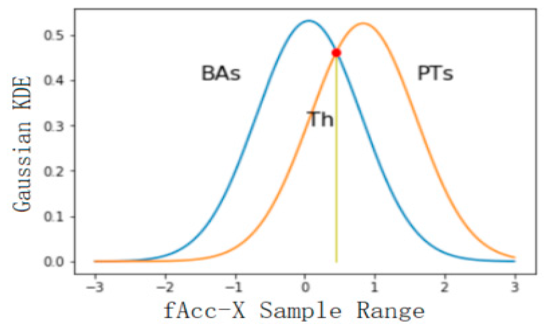
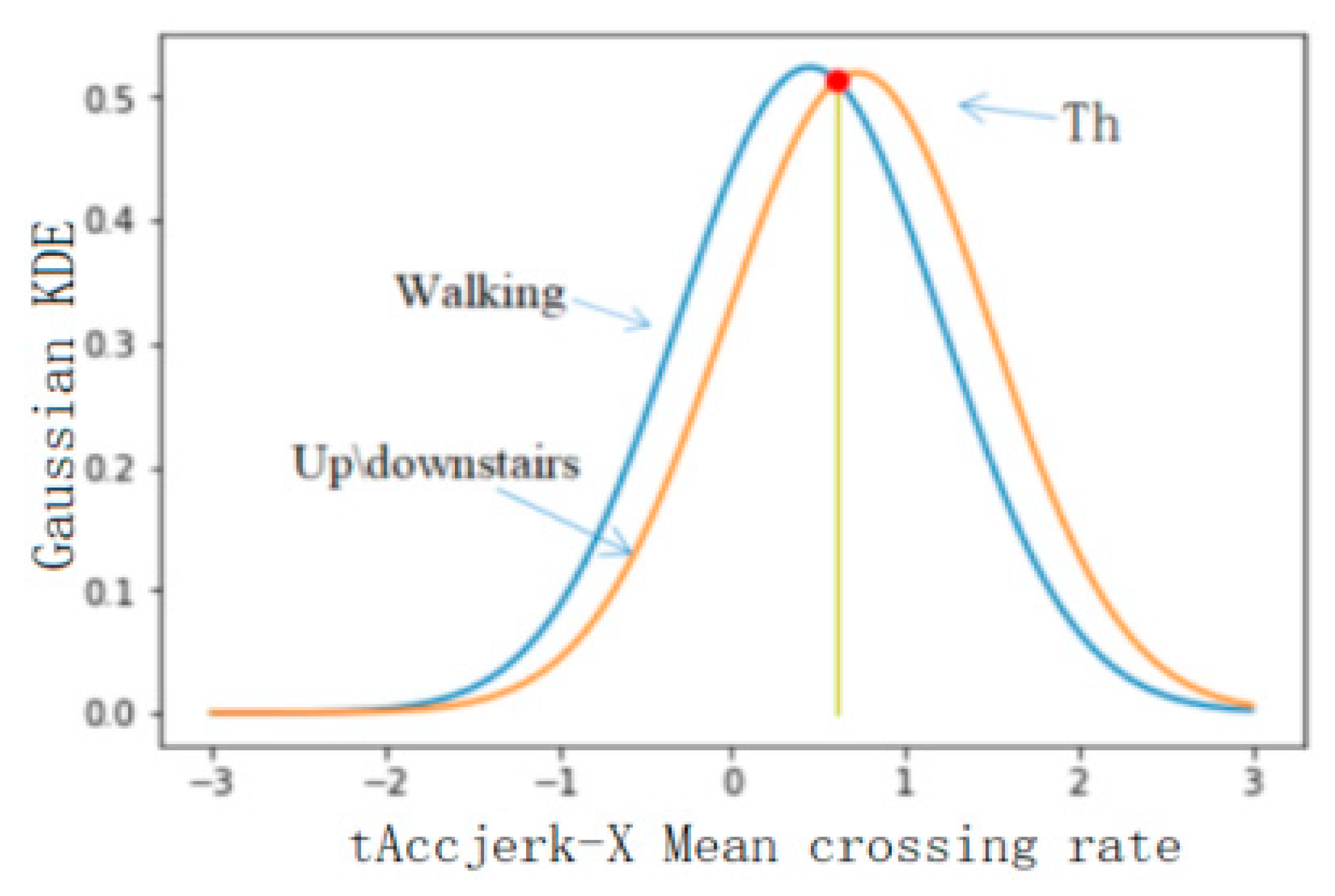
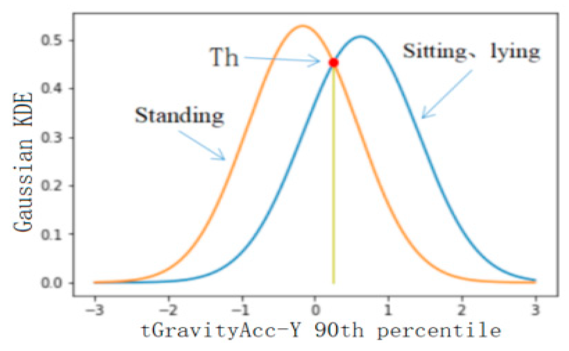
Using the feature set selected in the previous step as the feature used in threshold classification, the classification accuracy of the six levels was calculated, and the features with a better classification effect were selected for classification. In this study, 50% of the database data was used for threshold selection, and the rest of the data was used for precision verification. Firstly, the threshold value of BAs and PTs was selected, and the feature with the best classification effect was fAcc-X Sample Range. The probability distribution of static and dynamic actions is shown in Figure 5, where the calculated threshold is 0.045 and the classification accuracy is 0.91. The threshold value of static and dynamic actions was selected, and the feature with the best classification effect was the tAccMag 75th percentile. The probability distribution of static and dynamic actions is shown in Figure 6, where the calculated threshold is 0.024 and the classification accuracy is 0.99. Furthermore, the threshold value was selected for walking, going upstairs, and going downstairs, and the corresponding probability distribution was obtained by using the characteristic tAccJerk-X Mean crossing rate, as shown in Figure 7. The threshold value was determined to be 0.604, and the corresponding classification accuracy was 0.77. Therefore, it can be seen that the threshold classification is not ideal for walking, going upstairs, and going downstairs. In terms of using the feature tGyro-X 10th percentile to carry out threshold selection for going upstairs and going downstairs, the corresponding probability distribution diagram is shown in Figure 8. The calculated threshold was −0.699, and the classification accuracy was 0.97, thus it can be seen that the classification effect was relatively ideal. Using the tGravityAcc-Y 90th percentile to carry out threshold selection for standing, sitting, and lying, the corresponding probability distribution diagram was developed, as shown in Figure 9. The calculated threshold was 0.255 and the classification accuracy was 0.97, so the classification effect was relatively ideal. In the last step, using the tAcc-X 50th percentile to carry out threshold selection for sitting and lying, the corresponding probability distribution diagram was produced, as shown in Figure 10. The calculated threshold was 0.511 and the classification accuracy was 0.99, so the classification effect was relatively ideal.

5. Discussions

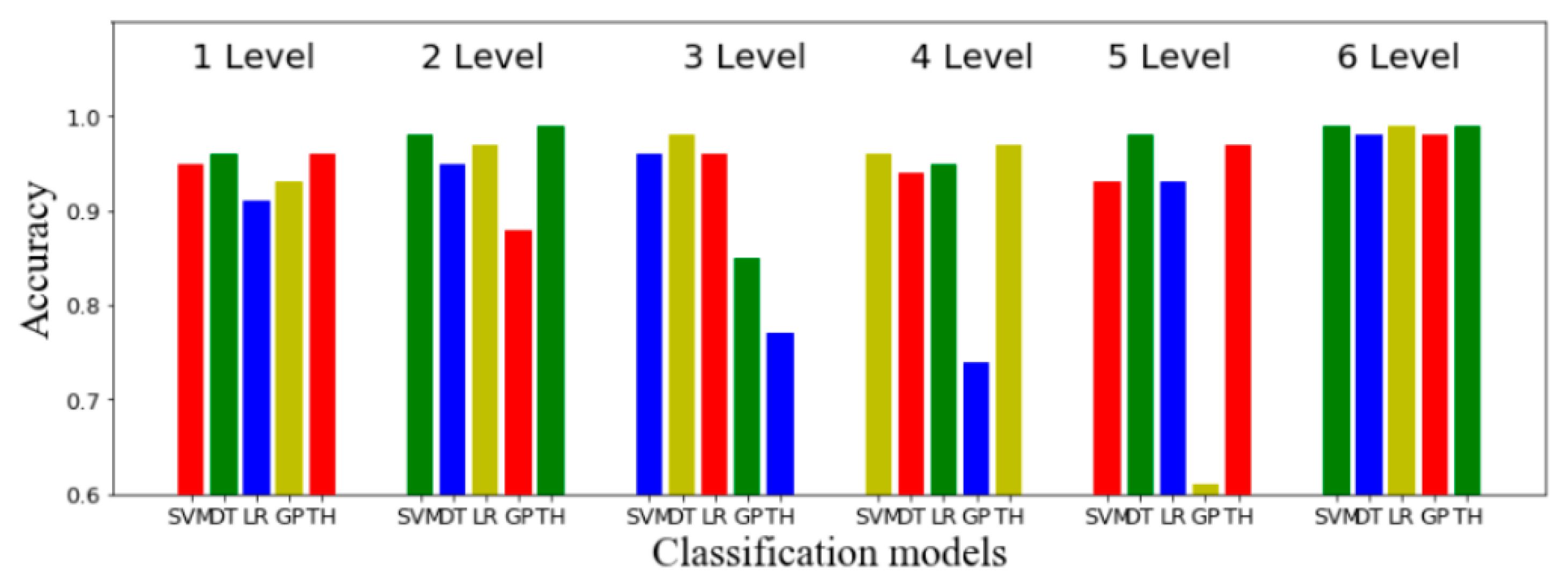
Multiple classification models (decision tree, linear regression, Gaussian process, and SVM) were used to further evaluate the accuracy of the classification at six levels, as shown in

Table 12. Accuracy of different levels of three classification models.

Level	SVM	DT	LR	GP	TH
One	0.98	0.96	0.97	0.89	0.91
Two	0.97	0.98	0.97	0.85	0.99
Three	0.97	0.94	0.96	0.74	0.77
Four	0.94	0.99	0.94	0.61	0.97
Five	0.94	0.99	0.93	0.68	0.97
Six	0.98	0.94	0.94	0.99	0.99

. The selected optimal feature set was input into the SVM classifier to train the classification model, and the 27th–29th people in the database were used for cross-validation to calculate the average precision value. It can be observed that the five classification levels can achieve a satisfactory classification effect. According to the experiments presented in the literature [44], when the proportion of the training data set is 70%~90%, the accuracy of the decision tree algorithm is relatively high, and the proportion of the training set selected in this paper was 70%. This method verifies the proportion of the best training set and test set corresponding to the SVM, linear regression, and the Gaussian process, and verifies that its classification accuracy can reach a high level through cross-validation. Figure 11 shows the total accuracy of classification for six BAs and PTs using SVM, a decision tree (DT), linear regression (LR), the Gaussian process (GP), and threshold classification (TH) in six levels. In general analysis, the method of threshold classification has a better effect. As shown in Figure 11, the classification accuracy of the five classifiers is higher in the fifth layer (that is, to distinguish between sitting and lying).

It can be seen from Table 12 that the feature selection method proposed in this paper, which uses different feature sets for classification at different levels based on SVM, can achieve better classification results when applied to the decision tree and linear regression classification model, but it is not applicable to the Gaussian process. It uses all selected feature sets in six levels of classification to classify six BAs and PTs. It can be seen from

Table 13. Confusion matrix for the simultaneous classification of six actions.

Class	WK	GU	GD	ST	SD	LY	PTs
WK	181	0	0	0	1	0	4
GU	5	174	7	0	0	0	1
GD	5	2	153	0	0	0	1
ST	5	0	0	186	3	0	5
SD	5	0	0	9	192	0	1
LY	6	0	0	0	0	207	1
PTs	6	1	5	4	1	0	38

that trained classifiers can obtain better classification results.

Finally, the data of the 22nd person in the database were used to simulate online prediction human activity recognition. According to Table 11 we decided to use SVM in the first level, TH in the second level, SVM in the third level, DT in the fourth level and fifth level, and TH in the sixth level. The experimental results are shown in Figure 12. The classification accuracy was 0.94. Nicole et al. [45] also used a similar feature selection algorithm, but only considered 76 features and verified them using different classification methods. In this work, 48 features were selected from 585 features, and the frequency domain characteristics were taken into account. The results show that the frequency domain characteristics apply to the first layer, the third layer, and the fifth layer classification. Since the orientation angle of the portable sensor is prone to error, it is finally found that Mag ($\sqrt{x^2+y^2+z^2}$) is more suitable for activity classification.

6. Conclusions

This paper proposes a feature selection method that synthesizes multiple feature selection algorithms and considers the combination effect among features. In order to verify this method, we calculated 585 features, including time and frequency domains, and used various classifiers, such as SVM, to evaluate the features selected by the introduced feature selection method, and the validity of the introduced feature has been verified. This paper used the threshold classification method, a decision tree, linear regression, and the Gaussian process to evaluate the classification accuracy of the selected features. The results show that the human activity recognition system based on an inertial sensor has a good classification effect on several human activities and can play a good auxiliary role in a human activity recognition system. The feature selection method works for many classification methods (SVM, TH, DT, LR, and GP). We finally classified the seven activities according to the method presented in

Table 14. Features selected and classifiers employed for each layer.

Level	The Features Selected	Classifier
1	fAcc-X-Sample Range, fAcc Largest Values	SVM
2	tAccMag-75th-Percentile	TH
3	tGyroJerk-Z-Sample-Variance, tAccMag-50th-Percentile, tGyro-X-50th-Percentile, tGyro-Y-Mean, tGyro-X-25th-Percentile, tGyro-X-Mean, tGyro-X-Median, tGyro-X-75th-Percentile, tGyro-X-10th-percentile, fGyro-X-Largest-values, tGyro-X-90th-Percentile, tAccMag-Skewness, tGyro-Y-Median, tGyro-X- 50th-Percentile, fAccJerk-Y-Smallest-value, tGyroMag-Skewness, tAccJerk-X-Samlpe-Variance, tGyroJerk-Z-Median, tGyroJerk-Z-50th-Percentile, tAccMag-Median, tAcc-X-Samlpe-Variance, tGyroJerk-Z-Skewness, tGyro-X-Skewness, fGyro-X-Smallest-value, tGyroJerk-Z-Power, Median-tGyroMag, tGyroMag-50th-percentile, fAccJerk-Y-Sample-Range, fAccJerk-Y-Largest-value, tGyroAng-Slope, tGyroAng-Kurtosis, tGyroJerk-Z-Root-Mean-Square, tAccJerk-X-Sample-Range, tGyroMag-Largest-values, tGyroMag-Power, tGyroAng-Power	SVM
4	tAccMag-10th-percentile, tGravityAccMag-10th-percentile	DT
5	tGravityAccMag-50th-Percentile, tGravityAcc-Y-Median, fAcc-Y-Smallest-value, fAcc-XLargest-values, fGyro-Z-Largest-values, fAccJerk-X-Largest-values	DT
6	tAcc-50th-Percentile	TH

. Compared to other classification methods, the method proposed in this paper can select a feature set with smaller dimensions and obtain higher classification accuracy. In the future, more classification activities and methods are needed to test the algorithm proposed in this paper. At the same time, we hope that IMU can better and more effectively assist the human activities recognition system.

References

- Lee, J.; Kim, J. Energy-Efficient Real-Time Human Activity Recognition on Smart Mobile Devices. Mob. Inf. Syst. 2016, 2016, 2316757. [Google Scholar] [CrossRef]
- Yang, R.; Wang, B. PACP: A Position-Independent Activity Recognition Method Using Smartphone Sensors. Information 2016, 7, 72. [Google Scholar] [CrossRef]
- He, Y.; Li, Y. Physical activity recognition utilizing the built-in Kinematic sensors of a smartphone. Int. J. Distrib. Sens. Netw. 2013, 9, 481580. [Google Scholar] [CrossRef]
- Qifan, Z.; Hai, Z.; Zahra, L.; Liu, Z.B.; Naser, E.S. Design and Implementation of Foot-Mounted Inertial Sensor Based Wearable Electronic Device for Game Play Application. J. Sens. 2016, 16, 1752. [Google Scholar]
- Robertas, D.; Mindaugas, V.; Justas, Š.; Marcin, W. Human Activity Recognition in AAL Environments Using Random Projections. Comput. Math. Methods Med. 2016, 2016, 4073584. [Google Scholar]
- Sorkun, M.C.; Danişman, A.E.; İncel, Ö.D. Human activity recognition with mobile phone sensors: Impact of sensors and window size. In Proceedings of the 2018 26th Signal Processing and Communications Applications Conference (SIU), Izmir, Turkey, 2–5 May 2018; pp. 1–4. [Google Scholar]
- Nurhazarifah, C.H.; Nazatul, A.A.M.; Haslina, A.; Waqas, K.O. User Satisfaction for an Augmented Reality Application to Support Productive Vocabulary Using Speech Recognition. Adv. Multimed. 2018, 2018, 9753979. [Google Scholar]
- Zheng, Y.H. Human Activity Recognition Based on the Hierarchical Feature Selection and Classification Framework. J. Electr. Comput. Eng. 2015, 2015, 140820. [Google Scholar] [CrossRef]
- Leonardis, G.D.; Rosati, S.; Balestra, G.; Agostini, V.; Panero, E.; Gastaldi, L.; Knaflitz, M. Human Activity Recognition by Wearable Sensors: Comparison of different classifiers for real-time applications. In Proceedings of the 2018 IEEE International Symposium on Medical Measurements and Applications (MeMeA), Rome, Italy, 11–13 June 2018; pp. 1–6. [Google Scholar]
- Jarraya, A.; Arour, K.; Bouzeghoub, A.; Borgi, A. Feature selection based on Choquet integral for human activity recognition. In Proceedings of the 2017 IEEE International Conference on Fuzzy Systems (FUZZ-IEEE), Naples, Italy, 9–12 July 2017; pp. 1–6. [Google Scholar]
- Doewes, A.; Swasono, S.E.; Harjito, B. Feature selection on Human Activity Recognition dataset using Minimum Redundancy Maximum Relevance. In Proceedings of the 2017 IEEE International Conference on Consumer Electronics—Taiwan (ICCE-TW), Taipei, Taiwan, 12–14 June 2017; pp. 171–172. [Google Scholar]
- Li, J. A Feature Subset Selection Algorithm Based on Feature Activity and Improved GA. In Proceedings of the 2015 11th International Conference on Computational Intelligence and Security (CIS), Shenzhen, China, 19–20 December 2015; pp. 206–210. [Google Scholar]
- Ridok, A.; Mahmudy, W.F.; Rifai, M. An improved artificial immune recognition system with fast correlation based filter (FCBF) for feature selection. In Proceedings of the 2017 Fourth International Conference on Image Information Processing (ICIIP), Shimla, India, 21–23 December 2017; pp. 1–6. [Google Scholar]
- Reyes-Ortiz, J.L.; Oneto, L.; Samà, A.; Xavier, P.; Davide, A. Transition-aware human activity recognition using smartphones. Neurocomputing 2016, 171, 754–767. [Google Scholar] [CrossRef]
- Zhang, T.; Zhang, Y.; Cai, J.; Kot, A.C. Efficient object feature selection for action recognition. In Proceedings of the 2016 IEEE International Conference on Acoustics, Speech and Signal Processing (ICASSP), Shanghai, China, 20–25 March 2016; pp. 2707–2711. [Google Scholar]
- San-Segundo, R.; Montero, J.M.; Barra-Chicote, R.; Fernando, F.; José, M.P. Feature extraction from smartphone inertial signals for human activity segmentation. Signal Process. 2016, 120, 359–372. [Google Scholar] [CrossRef]
- Gao, L.; Bourke, A.K.; Nelson, J. A comparison of classifiers for activity recognition using multiple accelerometer-based sensors. In Proceedings of the 2012 IEEE 11th International Conference on Cybernetic Intelligent Systems (CIS), Limerick, Ireland, 23–24 August 2012; pp. 149–153. [Google Scholar]
- Xie, L.; Tian, J.; Ding, G.; Zhao, Q. Human activity recognition method based on inertial sensor and barometer. In Proceedings of the 2018 IEEE International Symposium on Inertial Sensors and Systems (INERTIAL), Moltrasio, Italy, 26–19 March 2018; pp. 1–4. [Google Scholar]
- Rajesh, K.; Sugumaran, V.; Vijayaram, T.; Karthikeyan, C. Activities of daily life (ADL) recognition using wrist-worn accelerometer. Int. J. Eng. Technol. 2016, 8, 1406–1413. [Google Scholar]
- Nhan, D.N.; Duong, T.B.; Phuc, H.T.; Gu-Min, J. Position-Based Feature Selection for Body Sensors regarding Daily Living Activity Recognition. J. Sens. 2018, 2018, 9762098. [Google Scholar]
- Karantonis, M.D.; Narayanan, M.R.; Mathie, M.; Lovell, N.H.; Celler, B.G. Implementation of a realtime human movement classifier using a triaxial accelerometer for ambulatory monitoring. IEEE Trans. Inf. Technol. Biomed. 2006, 10, 156–167. [Google Scholar] [CrossRef] [PubMed]
- Mobark, M.; Chuprat, S.; Mantoro, T. Improving the accuracy of complex activities recognition using accelerometer-embedded mobile phone classifiers. In Proceedings of the 2017 Second International Conference on Informatics and Computing (ICIC), Jayapura, Indonesia, 1–3 November 2017; pp. 1–5. [Google Scholar]
- Albert, S.; Angulo, C.; Pardo, D.; Andreu, C.; Cabestany, J. Analyzing human gait and posture by combining feature selection and kernel methods. Neurocomputing 2011, 74, 2665–2674. [Google Scholar] [Green Version]
- Kaytaran, T.; Bayindir, L. Activity recognition with wrist found in photon development board and accelerometer. In Proceedings of the 2018 26th Signal Processing and Communications Applications Conference (SIU), Izmir, Turkey, 2–5 May 2018; pp. 1–4. [Google Scholar]
- Ho, J. Interruptions: Using activity transitions to trigger proactive messages. Master’s Thesis, Massachusetts Institute of Technology, Cambridge, MA, USA, 2004. [Google Scholar]
- Chen, C.; Jafari, R.; Kehtarnavaz, N. A real-time human action recognition system using depth and inertial sensor fusion. IEEE Sens. J. 2016, 16, 773–781. [Google Scholar] [CrossRef]
- Tao, D.; Jin, L.; Yuan, Y.; Xue, Y. Ensemble manifold rank preserving for acceleration-based human activity recognition. IEEE Trans. Neural Netw. Learn. Syst. 2014, 27, 1392–1404. [Google Scholar] [CrossRef] [PubMed]
- He, Z.; Jin, L. Activity recognition from acceleration data based on discrete consine transform and SVM. In Proceedings of the IEEE Conference on Systems, Man and Cybernetics, San Antonio, TX, USA, 11–14 October 2009; pp. 5041–5044. [Google Scholar]
- Wang, Z.; Wu, D.; Chen, J.; Ghoneim, A.; Hossain, M.A. A Triaxial Accelerometer-Based Human Activity Recognition via EEMD-Based Features and Game-Theory-Based Feature Selection. IEEE Sens. J. 2016, 16, 3198–3207. [Google Scholar] [CrossRef]
- Pourpanah, F.; Zhang, B.; Ma, R.; Hao, Q. Non-Intrusive Human Motion Recognition Using Distributed Sparse Sensors and the Genetic Algorithm Based Neural Network. In Proceedings of the 2018 IEEE SENSORS, New Delhi, India, 28–31 October 2018; pp. 1–4. [Google Scholar]
- Wang, L.; Gu, T.; Tao, X.P.; Chen, H.H.; Lu, J. Recognizing multi-user activities using wearable sensors in a smart home. Pervasive Mob. Comput. 2011, 7, 287–298. [Google Scholar] [CrossRef]
- Zhou, S.L.; Fei, F.; Zhang, G.L.; John, D.M.; Liu, Y.H.; Liou, J.Y.J.; Li, W.J. 2D Human Gesture Tracking and Recognition by the Fusion of MEMS Inertial and Vision Sensors. IEEE Sens. J. 2014, 14, 1160–1170. [Google Scholar] [CrossRef]
- Yang, M.; Chen, Y.; Ji, G. Semi_Fisher Score: A semi-supervised method for feature selection. In Proceedings of the 2010 International Conference on Machine Learning and Cybernetics, Qingdao, China, 11–14 July 2010; pp. 527–532. [Google Scholar]
- Liu, X.; Wang, X.L.; Su, Q. Feature selection of medical data sets based on RS-RELIEFF. In Proceedings of the 2015 12th International Conference on Service Systems and Service Management (ICSSSM), Guangzhou, China, 22–24 June 2015; pp. 1–5. [Google Scholar]
- Haryanto, A.W.; Mawardi, E.K.; Muljono. Influence of Word Normalization and Chi-Squared Feature Selection on Support Vector Machine (SVM) Text Classification. In Proceedings of the 2018 International Seminar on Application for Technology of Information and Communication, Semarang, Indonesia, 21–22 September 2018; pp. 229–233. [Google Scholar]
- Dai, H. Research on SVM improved algorithm for large data classification. In Proceedings of the 2018 IEEE 3rd International Conference on Big Data Analysis (ICBDA), Shanghai, China, 9–12 March 2018; pp. 181–185. [Google Scholar]
- Alam, S.; Moonsoo, K.; Jae-Young, P.; Kwon, G. Performance of classification based on PCA, linear SVM, and Multi-kernel SVM. In Proceedings of the 2016 Eighth International Conference on Ubiquitous and Future Networks (ICUFN), Vienna, Austria, 5–8 July 2016; pp. 987–989. [Google Scholar]
- Zhou, Y.; Cheng, Z.; Jing, L. Threshold selection and adjustment for online segmentation of one-stroke finger gestures using single tri-axial accelerometer. Multimed. Tools Appl. 2015, 74, 9387–9406. [Google Scholar] [CrossRef]
- Bulling, A.; Blanke, U.; Schiele, B. A tutorial on human activity recognition using body-worn inertial sensors. Acm Comput. Surv. 2013, 46, 33. [Google Scholar] [CrossRef]
- Hoai, M.; Torre, F.D.L. Maximum margin temporal clustering. In Proceedings of the 25th IEEE Conference on Computer Vision and Pattern Recognition, Providence, RI, USA, 18–20 June 2012. [Google Scholar]
- Kavitha, S.; Varuna, S.; Ramya, R. A comparative analysis on linear regression and support vector regression. In Proceedings of the 2016 Online International Conference on Green Engineering and Technologies (IC-GET), Coimbatore, India, 19 November 2016; pp. 1–5. [Google Scholar]
- Liu, X.; Zhang, J. Active learning for human action recognition with Gaussian Processes. In Proceedings of the 2011 18th IEEE International Conference on Image Processing, Brussels, Belgium, 11–14 September 2011; pp. 3253–3256. [Google Scholar]
- Oh, J.; Kim, T.; Hong, H. Using Binary Decision Tree and Multiclass SVM for Human Gesture Recognition. In Proceedings of the 2013 International Conference on Information Science and Applications (ICISA), Suwon, Korea, 24–26 June 2013; pp. 1–4. [Google Scholar]
- Yazdansepas, D.; Niazi, A.H.; Gay, J.L.; Maier, F.W.; Ramaswamy, L.; Rasheed, K.; Buman, M.P. A Multi-featured Approach for Wearable Sensor-Based Human Activity Recognition. In Proceedings of the 2016 IEEE International Conference on Healthcare Informatics (ICHI), Chicago, IL, USA, 4–7 October 2016; pp. 423–431. [Google Scholar]
- Capela, N.; Lemaire, E.; Baddour, N. Feature Selection for Wearable Smartphone-Based Human Activity Recognition with Able bodied, Elderly, and Stroke Patients. PLoS ONE 2015, 10. [Google Scholar] [CrossRef] [PubMed]
Figure 1.
Human activity recognition framework.
Figure 2.
Example of inertial signals from the accelerometer while performing six activities.
Figure 3.
Example of inertial signals from the gyroscope while performing six activities.
Figure 4.
The comparison of the classification accuracy and the number of selected features in the six layers. The first layer: basic activities and postural transitions (a); the second layer: static state and dynamic state (b); the third layer: walking, going upstairs, and downstairs (c); the fourth layer: going upstairs and downstairs (d); the fifth layer: standing, sitting, and lying (e); and the sixth layer: sitting and lying (f).
Figure 5.
Probability distribution of basic activities (Bas) and postural transitions (PTs).
Figure 6.
Probability distribution of static and dynamic action.
Figure 7.
Probability distribution of walking and up-downstairs.
Figure 8.
Probability distribution of upstairs and downstairs.
Figure 9.
Probability distribution of standing, sitting, and lying.
Figure 10.
Probability distribution of sitting and lying.
Figure 11.
Accuracy for six activities using multiple classification approaches.
Figure 12.
The actual label of the 22nd person (a), and the simulated online prediction of the 22nd person (b). The label of walking (WK) is “1”, the label of walking upstairs (WU) is “2”, the label of walking downstairs (WD) is “3”, the label of standing (SD) is “4”, the label of sitting (ST) is “5”, the label of lying (LY) is “6”, and the label of PTs is “7”.