Climate Action Gaming Experiment: Methods and Example Results

Abstract

An exercise has been prepared and executed to simulate international interactions on policies related to greenhouse gases and global albedo management. Simulation participants are each assigned one of six regions that together contain all of the countries in the world. Participants make quinquennial policy decisions on greenhouse gas emissions, recapture of ${\mathrm{CO}}_2$ from the atmosphere, and/or modification of the global albedo. Costs of climate change and of implementing policy decisions impact each region’s gross domestic product. Participants are tasked with maximizing economic benefits to their region while nearly stabilizing atmospheric ${\mathrm{CO}}_2$ concentrations by the end of the simulation in Julian year 2195. Results are shown where regions most adversely affected by effects of greenhouse gas emissions resort to increases in the earth’s albedo to reduce net solar insolation. These actions induce temperate region countries to reduce net greenhouse gas emissions. An example outcome is a trajectory to the year 2195 of atmospheric greenhouse emissions and concentrations, sea level, and global average temperature.

1. Introduction

A U.S. National Research Council (NRC) study has concluded that anthropogenic modification of the earth’s albedo is a not unlikely response to growing impact of climate change [1]. The Intergovernmental Panel on Climate Change (IPCC) has estimated the probability of impacts of climate change resulting from various levels of emissions of greenhouse gases, but without accounting for anthropogenic albedo management in the scenarios used [2]. Neither the NRC nor the IPCC reports were designed to estimate the probability of actual outcomes for climate change, with or without albedo modification. This limitation is problematic for those involved in land use planning, management of aquatic environments, and a variety sectors likely to be impacted by climate change, as they are currently left with little guidance on the probability of actual likely outcomes for climate change.

Carbon and nitrogen cycle models that account for biological activities of numerous species [3,4] generally do not explicitly model the expected feedback of increased greenhouse gas concentrations on human actions that are driving rapid changes in those concentrations. For example, the feedback effect of changes in temperature and atmospheric ${\mathrm{CO}}_2$ concentration on the rate of photosynthesis by various species is accounted for in a global carbon cycle model of Eliseev and Mokhov [5]; but how the species Homo sapiens might respond to such changes in ways that also produce feedback effects on ${\mathrm{CO}}_2$ emissions is not included in those authors’ model. The present paper thus presents methodology and example results of an experimental approach to quantifying the impact of climate change on human decisions about net greenhouse gas emissions and albedo management.

A simulation is described here that uses results of an interactive exercise to modify a reference set of future conditions that are based upon extrapolation of historical trends. The simulation exercise models physical environmental response, economic impact, and interactions between participants as each participant makes policy decisions affecting greenhouse gas emissions and the global albedo. In the simulation, participants represent different groups of countries (with these groups here called regions) and attempt to maximize their economic gains while dealing with a changing climate. This approach provides an experimental framework for investigating outcomes for human influences on future climate change. Simple by design compared to complex global circulation models, this simulation is neither a prediction of the future nor a method of policy prescription. Rather, it presents a new way to look at a complex problem that involves both natural science and human factors.

The basic setup of the model divides the world into six regions and extrapolates each region’s gross domestic product (GDP) and population into the future in a manner consistent with extensive historical time-series data [6,7,8,9,10,11,12,13,14,15,16]. A fraction of each region’s GDP is diverted to that region’s “pot balance”, which is used to determine scoring in the simulation game. Direct costs of albedo management and of reductions in net greenhouse gas emissions are charged to each pot balance, as are costs of impacts from climate change.

Managers of each simulation can adjust model parameters to investigate how different assumptions (e.g., a higher estimated cost of sea-level rise or new research and development lowering the cost of reducing greenhouse gas emissions) affect participants’ behavior and the ultimate outcome. A complete description of the simulation model is given as an appendix in Section 4 below. Tabular and in-text values of reference values for subscripted symbols in Section 4 define the reference model behind the results described here.

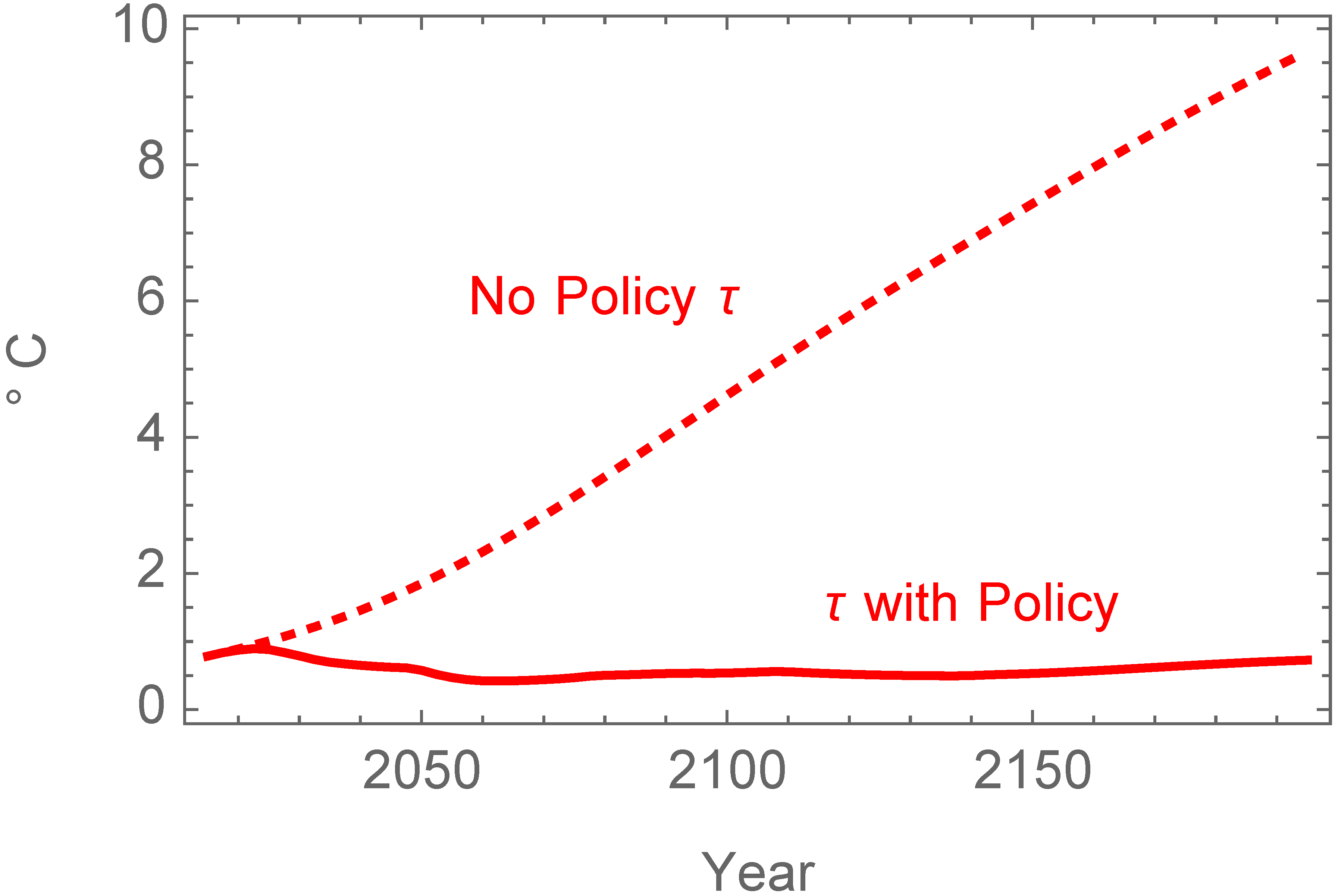
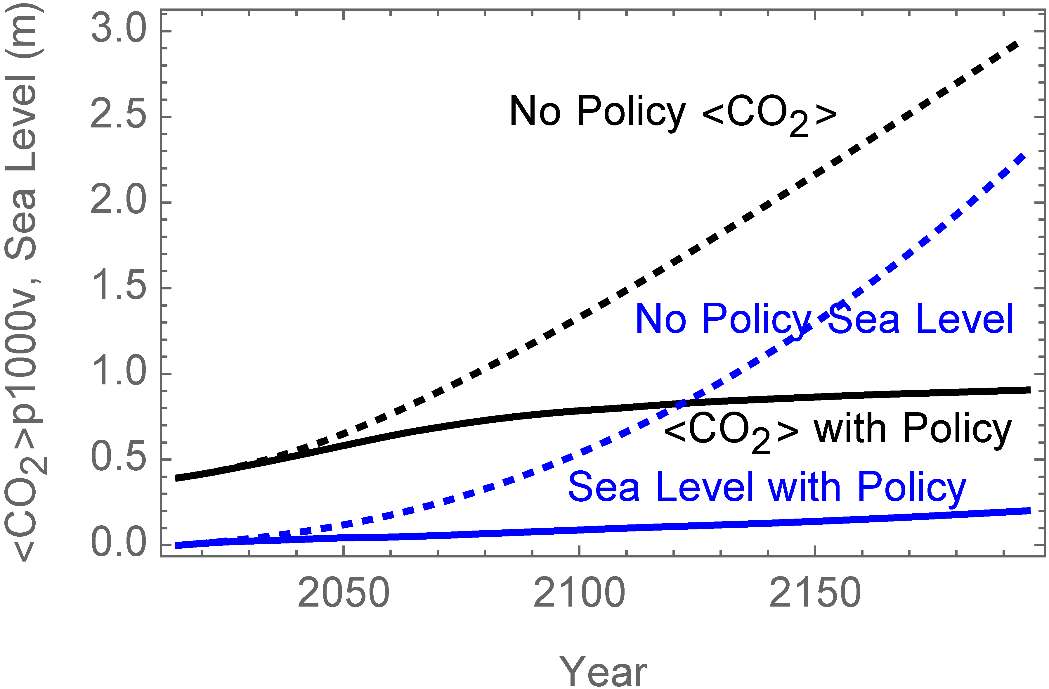
If participants take no actions, in the year 2195 the atmospheric ${\mathrm{CO}}_2$ concentration in parts per million by volume (ppmv) reaches 2876, the global average temperature has increased by 9.5 °C above the preindustrial reference level listed below in Table 3, and sea level has risen 217 cm over its 2015 value. Figure 1 and Figure 2 compare these outcomes to one set of results following from participants’ decisions, as discussed in Section 2.6.

Figure 1. Industrial era global average temperature increment, τ, from 2015 to 2195 with (solid curve) and without (dashed curve) participants’ policy decisions.

Figure 1. Industrial era global average temperature increment, τ, from 2015 to 2195 with (solid curve) and without (dashed curve) participants’ policy decisions.

2. Methods and Example Results

This section summarizes simulation methods. This summary is followed by a description of results of a simulation exercise by groups of undergraduate students at the University of Illinois at Urbana-Champaign. The simulation described here was preceded by ten previous ones, mostly done with inadequate time provided for thorough discussions amongst participants. Some of these gave similar results to the one described here, while in others participants made little progress in limiting the increase of global average temperature. For simplicity then, just a single simulation conducted in three separate one hour segments is described.

Figure 2. Atmospheric ${\mathrm{CO}}_2$ concentrations in parts per thousand by volume, and increase of sea level over its 2015 value, with (solid curves) and without (dashed curves) participants’ policy decisions.

Figure 2. Atmospheric ${\mathrm{CO}}_2$ concentrations in parts per thousand by volume, and increase of sea level over its 2015 value, with (solid curves) and without (dashed curves) participants’ policy decisions.

2.1. Extrapolation of Historical Trends

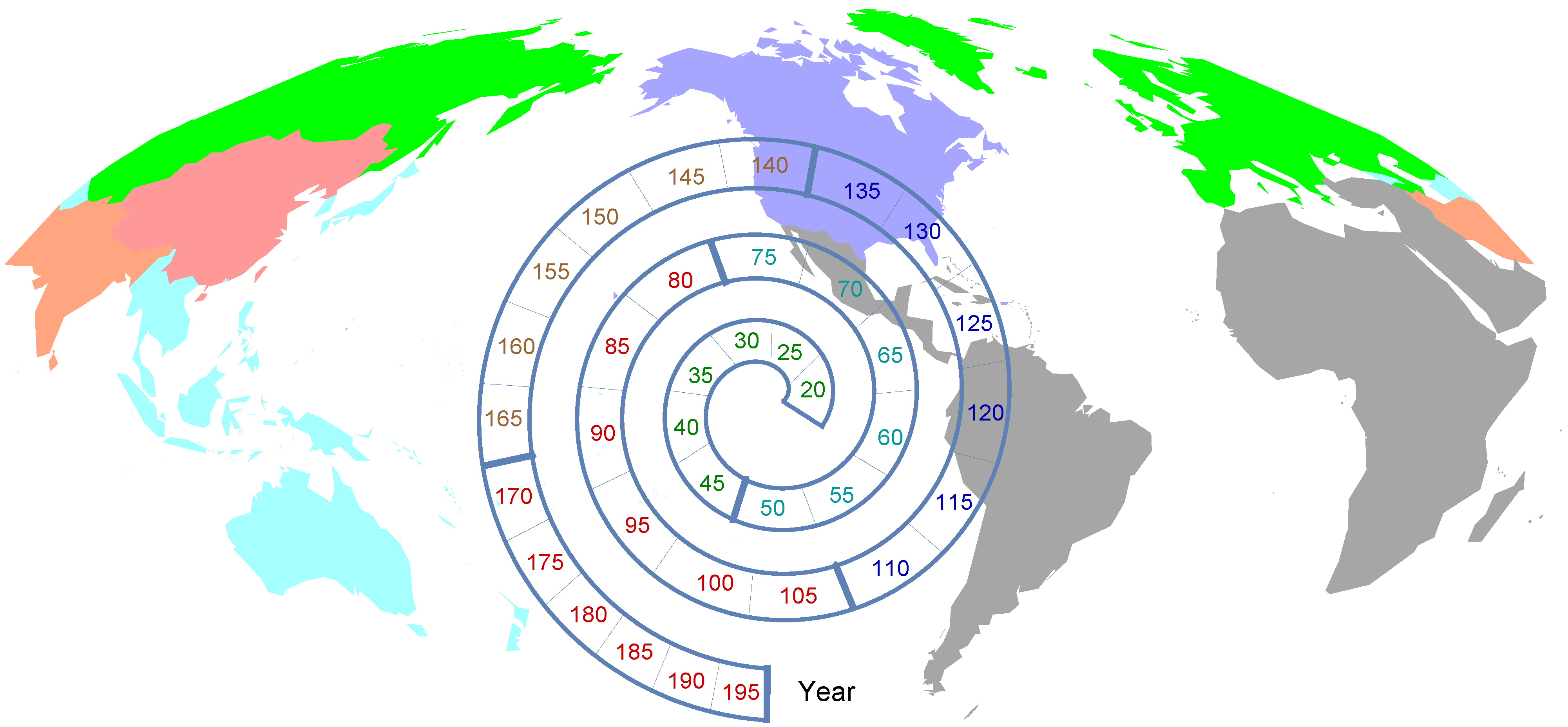
This subsection describes a reference case extrapolation of historical data, which serves as the basis for the simulation. The simulation begins by dividing the world into six regions: China+, US+, EU+, India+, Oceania, and G121. The G121 group consists of Latin America, Africa, and the Middle East (cf. Figure 3). The spiral in Figure 3 in indicates the times, in years from Julian year 2000, when quinquennial decisions on greenhouse gases and albedo manangement are made by participants. A moderator entered the numbers corresponding to these decisions sequentially into an Excel spreadsheet in the order of the six regions listed above. The temporally latest entries are carried down to year 2195, which is equivalent to an assumption that the latest policy decisions will be carried forward ad infinitum. The spreadsheet, which was visible on a projection screen, updates upon each entry to allow participants to see the impact of each decision on the future of global average temperature, atmospheric ${\mathrm{CO}}_2$ concentration, and sea level, and on the economic status of each region as described below. Participants had an opportunity to interact verbally at any point in the process. The moderator was requested to encourage participants to converse about their decisions but not to recommend policy decisions.

An overview of the steps simulation exercise process is as follows:

• Provide participants with a written and/or oral description of the model used.

• Assign participants to regions and choose a simulation moderator.

• Have the participants decide on the first round of policy decisions (for year 2020).

• Evolve the nitrous oxide and fluorine compounds atmospheric concentrations to 2195.

• Evolve the coupled global heat and carbon balances to 2195.

• Evolve the global land ice balance to 2195 and compute sea level change.

• Evolve each region’s economic “pot balance” as described below.

• Present the results to the participants and repeat the process until 2195.

• Discuss the final results with the participants.

Steps 4–8 are executed together in an Excel spreadsheet, using a simple Euler solution method for steps 4–6 and a time step of 2.5 years, with the entire process taking about one second on a MacBook Pro laptop. Thus, most of the actual simulation time is taken up with discussions in steps 3 and 9, which require together about three hours unless the moderator imposes more stringent time limits on the participants’ policy decision reporting. The participants have the option of all agreeing at any point to carry forward their latest policy decisions out to 2195, which can reduce the total time needed for the simulation.

Figure 3. Map of six regions used. The spiral indicates decision times in years after Julian year 2000, with bold lines at the end of the 30-year “generations” when participants are tasked with having positive pot balances.

Figure 3. Map of six regions used. The spiral indicates decision times in years after Julian year 2000, with bold lines at the end of the 30-year “generations” when participants are tasked with having positive pot balances.

The reference case includes extrapolations of each region’s historical gross domestic product (GDP), along with extrapolation of emissions of ${\mathrm{CO}}_2$, ${\text{N}}_2$O, and volatile fluorine compounds. Other greenhouse gas emissions were not included because it was assumed that changes in their contribution to radiative forcing will be small enough to be overshadowed by policies affecting these three categories of greenhouse gas. In particular, future increases in atmospheric methane concentrations were not accounted for. When the simulation was formulated for exploratory exercises with different sets of participants, atmospheric methane concentrations had recently nearly stabilized for about eight years, but since then atmospheric methane content started increasing again. Eventually, the much longer atmospheric lifetime of nitrous oxide may make it a more important greenhouse gas than methane, but it may become apparent over the next few years that a model of atmospheric methane concentrations should also be included in the simulation.

Reference ${\mathrm{CO}}_2$ emissions for each region were estimated by multiplying the amount of energy a region was expected to use, extrapolated over time, by the extrapolated carbon intensity of energy use. The extrapolated populations for countries or groups of countries in each region were added to form a reference case estimate for the evolution of global population. For details on methods used for extrapolation of population, GDP, energy use rates, and ratios of carbon emissions rates to energy use rates (i.e., carbon intensity), see Singer et al. [17]. In that work, the increase of population in each region over a year 1820 base level was fit with a logistic function. (A logistic function initially grows exponentially, increases linearly at the point of its half maximum, and then approaches a maximum value with the difference between that maximum value and the function eventually decaying exponentially.) The increase of GDP over a year 1820 levels was fit with a utility maximization model that had a logistic productivity function; so the GDP also asymptotically approaches a maximum.

Fossil fuel resources, including coal and unconventional natural gas and oil [18], are assumed to be large enough to allow higher than zero carbon intensity of energy production in the absence of new policy decisions limiting carbon burning for the duration of the time covered by the simulation. It should be noted that, in the extrapolations of carbon intensity of energy production, the difference between the carbon intensity of all-coal commercial energy use and a long term limit carbon intensity declines exponentially with cumulative carbon use in each region, and this decline in some cases is in part a result of pre-existing national policies. Thus, the “no policy” extrapolations referred to here are most accurately described as involving “no new policy” decisions by simulation participants beyond those already accounted for in extrapolation of historical trends.

Anthropogenic increases in ${\text{N}}_2$O emissions result primarily from use of agricultural fertilizers. Fertilizer that is not taken up by plants is metabolized by organisms in soil or water, leading to the release of ${\text{N}}_2$O. Since the majority of the world’s agriculture focuses on the production of the eight major cereal grains (rice, wheat, maize, barley, sorghum, millet, oats, and rye), this simulation uses each region’s production of these grains, as a fraction of total world production, to estimate their contribution to global ${\text{N}}_2$O emissions, cf. [19,20]. This approach implicitly assumes that over time the current fractions of the world’s cereal grains grown in each of the six regions remain constant. If the players take no action, ${\text{N}}_2$O emissions increase in proportion to global population growth.

A variety of fluorine compounds act as greenhouse gasses. Releases include refrigerants not recycled, foam blowing agents, and compounds used for other industrial processes (which include ${\text{CF}}_4$, ${\text{C}}_2{\text{F}}_6$, and ${\text{SF}}_6$ with very long atmospheric lifetimes [2]). The compounds included in this model and their atmospheric residence times are listed in Section 4.1. For the purposes of this simulation, the net effect of anthropogenic increases in methane concentrations and secular trends in the solar radiation balance other than periodic oscillations in incident solar irradiance are approximated as having already been stabilized by 2015.

2.2. Cost of Changing Emissions Levels

For reductions of greenhouse gas emissions, participants make decisions in the form of a percent reduction (e.g., a 5% reduction indicates the region is emitting 95% of reference case values). The cost for implementing these reductions is subtracted from each participant’s pot balance.

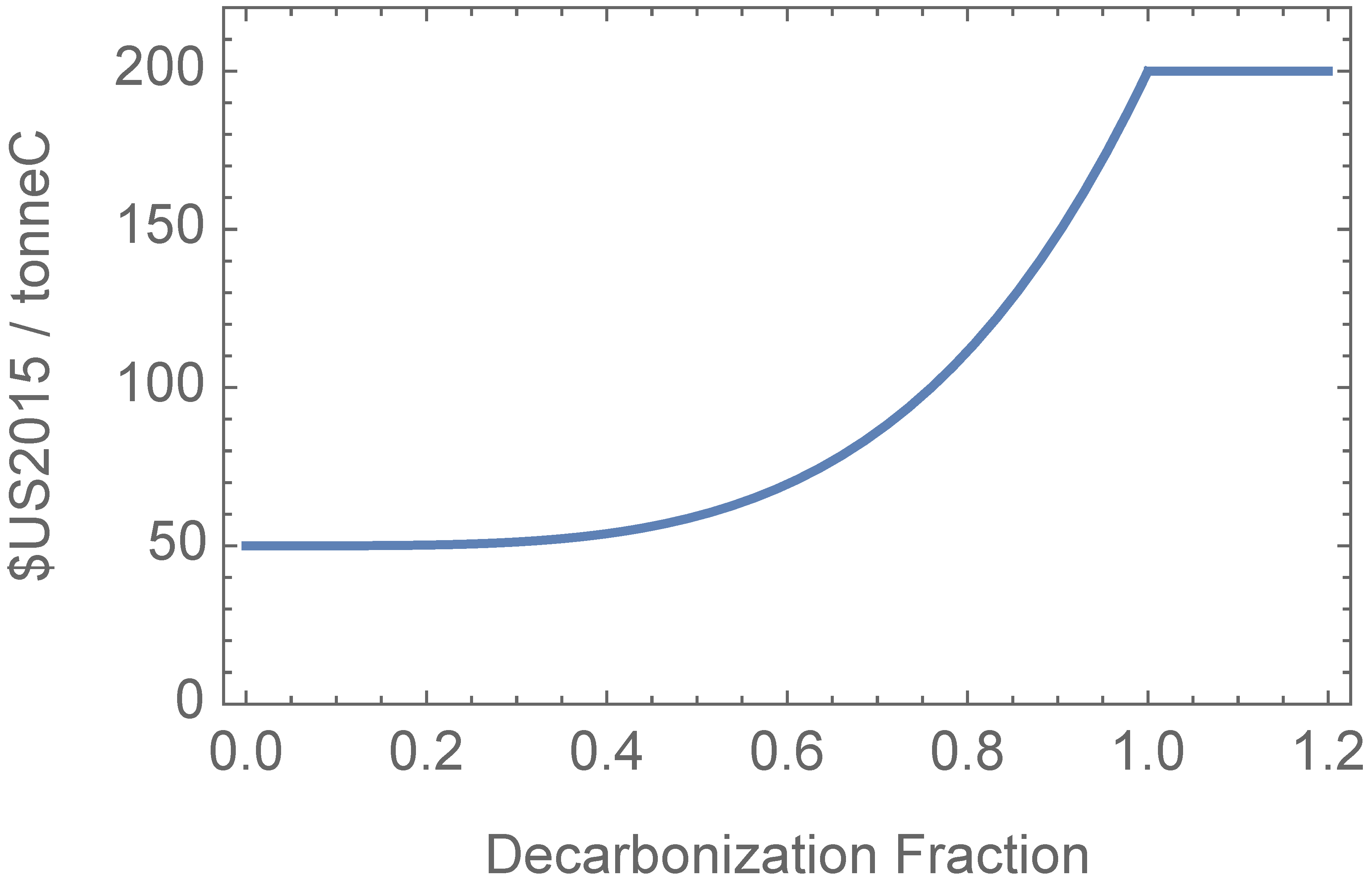
The costs for reductions in ${\text{CO}}_2$ emissions depend on energy decarbonization fractions. It is relatively cheap to achieve a small decarbonization fraction by replacing carbon intensive fuels such as coal with less carbon intensive fuels such as natural gas; but after about 60% decarbonization is reached the cost of further decarbonization increases steeply (see Figure 4). There is also a cost associated with rapid buildup of carbon emissions, as described in Section 4.2.

Figure 4. Average cost per metric ton of energy decarbonization as a function of decarbonization fraction.

Figure 4. Average cost per metric ton of energy decarbonization as a function of decarbonization fraction.

To reach levels of decarbonization exceeding 100%, it is possible to chemically sequester carbon after its release into the atmosphere [21,22], resulting in costs as illustrated on the horizontal line on the right hand side of Figure 4. Participants can also choose to use biosequestration in the form of biochar and other methods of immobilizing biological carbon [23]. However, the rate of biosequestration is limited by each region’s arable land area, as discussed in Section 4.1.

If a region has already reached a high level of energy decarbonization, it may become at least temporarily more cost effective for it to offer to pay for part of another region’s decarbonization, in lieu of some of the further reductions in its own carbon emissions. A simple implementation of this option used here allows each of the three initially high per capita ${\text{CO}}_2$, emitters, China+, USA+ and EU+, to pay half of the cost for augmenting reductions in the carbon emissions of exactly one other region, namely Ocean, India+, and G121 respectively.

The cost for reducing anthropogenic ${\text{N}}_2$O emissions increases quadratically with the emissions reduction fraction. This assumption is consistent with the idea that agriculture is the dominant source anthropogenic ${\text{N}}_2$O emissions, and that net proceeds from application of nitrogen fertilizers are a quadratic function of the amount of ${\text{N}}_2$O emissions [24]. The cost of reducing emissions of volatile fluorine greenhouse gas compounds is assumed to be a linear function of the reduction amounts. Equations for each can be found in Section 4.

2.3. Direct Costs of Solar Radiation Management

Participants also have the option of implementing up to three albedo management techniques to reduce the amount of sunlight that reaches the earth’s surface, thereby cooling the planet and helping offset warming caused by the greenhouse effect. These options include injection of sulfur into the stratosphere either globally or in a localized stratospheric arctic area, or low altitude lofting of salt water to create clouds [1,25,26,27,28]. The equations describing the costs for each of these methods are included in Section 4.2.

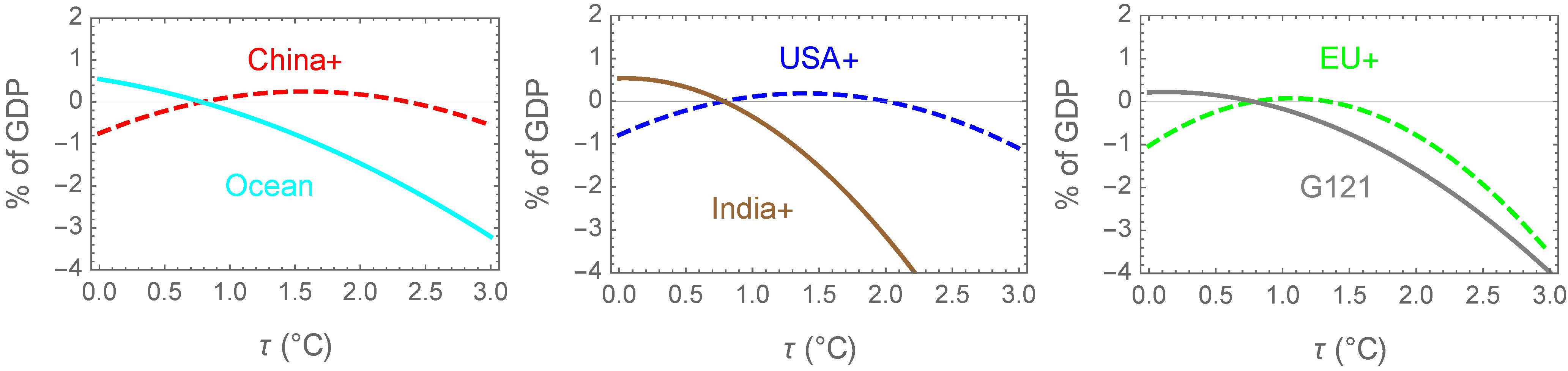
If a region chooses to inject sulfur into the stratosphere globally, that region alone will incur the direct costs of the process, but the resulting drop in global temperature will affect the pot balances of all of the regions in the simulation (cf. [30,31]). This differential effect is primarily a function of latitude, with more temperate regions (China+, USA+, and EU+) having higher optimum steady state temperatures than the other regions. Tropical and subtropical countries have lower optimum steady state temperatures, giving them an incentive to decrease the temperature significantly, through albedo management. However, overcooling of the earth has significant negative impacts on the economies of the China+, US+, and EU+ regions (cf. Figure 5).

Figure 5. Change in gross domestic product (GDP) in each region vs. global average temperature.

Figure 5. Change in gross domestic product (GDP) in each region vs. global average temperature.

Injecting sulfur into the arctic stratosphere also effects global average albedo, but at greater cost for the same amount of impact on global average temperature. However, arctic stratospheric sulfur injection could preferentially increase albedo over the arctic ice sheets, reducing land ice melting, and thus benefiting the Ocean and India+ regions that are assumed to be particularly sensitive to increases in sea level.

The other solar radiation management option presented to participants is low altitude salt water lofting, which seeds cloud formation. The clouds reflect sunlight, cooling the earth. Low altitude seawater lofting can increase rainfall along the coast in arid regions but reduce rainfall elsewhere. The expected economic impact of shifting rainfall patterns is not well known and is not included in the simulation exercise.

Participants’ decisions on emissions reductions and solar radiation management contribute to the global heat balance, global greenhouse gas concentrations, and global sea level change, all of which change throughout the simulation as participants make policy decisions. These values in turn affect each participant’s pot balance. Section 4.1 gives the equations used for this part of the model, which is described in qualitative terms here.

2.4. Global Physical Balances

The global heat balance accounts for thermal inertia of a 335-meter deep ocean surface layer and the difference between insolation (minus reflected energy) and thermal emission. The global average albedo decreases with increasing global average temperature, and increases with implementation of solar radiation management, cf. [32]. The thermal emissivity decreases with the net effect of increasing global average temperature on atmospheric water and with increasing concentrations of anthropogenic greenhouse gases. In light of ocean thermal inertia, solar insolation variations on 11 and 22-year cycles are neglected, but the effects of an 88 year Gleisburg cycle, and an assumed 600 year cycle with a minimum c. 1700, are included [17,33,34,35].

The rate of change in the amount of carbon dioxide in the atmosphere depends on anthropogenic emissions, the amount of carbon dioxide already present, and the global average temperature [17,33]. These dependences occur in large part because the surface ocean layer can absorb a fraction of global carbon emissions, but this fraction decreases over time if the oceans become more acidic, warmer, or both.

The concentrations of nitrous oxide and volatile fluorine compounds in the atmosphere at a given time during the simulation depend on extrapolated anthropogenic sources and removal rates proportional to increases over preindustrial concentration levels. Nitrous oxide is assumed to have a preindustrial concentration of 270 ppbv (parts per billion by volume), while volatile fluorine compounds are assumed to have preindustrial concentrations with negligible effect on net insolation [2]. The compounds included in the simulation and their atmospheric lifetimes are described in Section 4.1.

The model includes estimates of sea level change due to thermal expansion and melting of northern hemisphere land ice. The rate of land ice melting depends on global average temperature, the volume of land ice (and thus the average height of land ice and its surface temperature), and the amount of arctic stratospheric sulfur injection. The net effects of land ice melting and changes in precipitation in Antarctica [2,36] are less well understood and are not included.

2.5. Fund Balances

Throughout the simulation, participants have their current and extrapolated pot balances updated with every policy decision input. The extrapolations assume that the most recently entered policy decisions are carried forward until the last quinquennium before the end of the twenty-second century. Fund balances are affected by changes in global average temperature, by sea level and atmospheric ${\text{CO}}_2$ concentrations, and by the costs of emissions reductions and solar radiation management measures. Increases in atmospheric ${\text{CO}}_2$ levels over preindustrial values decrease pot balances even if global average temperature is held constant, due to direct effects on human physiology [37] and other environmental effects including ocean acidification. In addition to these changes, the participants’ pot balances accrue interest over time. Negative balances are charged interest, which can make it difficult to ever recover from a substantially negative pot balance.

Participants were instructed that successful completion of their contribution to the simulation exercise involved achieving the maximum end pot balance for their own region, subject to a constraint of no negative pot balance for their region at the end of each previous 30-year period and a limit of 1 ppmv/year change in atmospheric ${\text{CO}}_2$ concentration from 2190 to 2195. These instructions were designed to provide an incentive to emphasize approaching a state of environmental sustainability at minimum cost in the long term, but not at the expense of nearer term costs of policies that might be politically infeasible to implement.

If participants choose to inject sulfur into the stratosphere globally, the resulting global haze will interfere with astronomy and solar thermal electric energy systems but may increase solar to chemical energy conversion by some photosynthetic organisms. The net costs associated with these impacts are hard to quantify with information that is presently available. A small net globally distributed cost included in the current version of the simulation serves mostly as a placeholder until the implications of these effects can be studied in more depth.

2.6. A Six Region Simulation Exercise

After ten other trial runs, a simulation as described in the previous five sections was run in sequential discussion sections of two different undergraduate classes at the University of Illinois at Urbana-Champaign. The classes were comprised primarily of junior and senior level students with a broad mix of undergraduate majors. The results presented here are an example of how the simulation can be employed to study the human and scientific factors that may affect global climate change negotiations.

This simulation used the following percentages of each region’s annual GDP as inputs to its pot balance: China+ 1.12, USA+ 0.84, EU+ 0.76, Ocean 1.42, India+ 1.24, and G121 1.02. These fractions were assigned to make it possible but not easy for each region to maintain a positive balance throughout the simulation without resorting to global albedo management. Some of the other parameter values that differ from region to region are listed in Table 1. Ocean and India+ are the only regions with higher values for susceptibility to sea level rise, in order to simulate the vulnerability of low-lying parts of the Ocean region and of Bangladesh in the India+ region to higher sea levels. “Biochar...” in Table 1 refers to the sum of all processes of net carbon biosequestration.

Table 1. Region dependent parameters.

Parameter	China+	USA+	EU+	Ocean	India+	G121
Relative Sea Rise Cost	1	1	1	3	3	1
Max GtC/yr Biochar...	0.11	0.22	0.13	0.22	0.32	0.88

Table 1. Region dependent parameters.

Parameter	China+	USA+	EU+	Ocean	India+	G121
Relative Sea Rise Cost	1	1	1	3	3	1
Max GtC/yr Biochar...	0.11	0.22	0.13	0.22	0.32	0.88

In this simulation, the policies for reducing emissions of four volatile fluorine compounds that are used as refrigeration agents were fixed before the simulation began so that they reduced the no-policy emissions by 20% every five years until the reduction reached 80%, with the reduction set to 95% after another five years and remaining fixed thereafter. Reductions of emissions of ${\text{CF}}_4$, and ${\text{C}}_2{\text{F}}_6$, and ${\text{SF}}_6$, which have atmospheric lives of 2600 years or more, were incremented by 20% in each of the first five quinquennia. Leaving reducing emissions of the other three volatile fluorine compounds (listed in Section 4.2) included in the simulation to policy decisions brings the relevance of volatile fluorine compounds to the attention of participants while avoiding the distraction of multiple decisions on different classes of such compounds and avoiding a final state where the atmospheric concentrations of very long lived fluoine compounds are still building up without effective limits. In the example situation, participants reduced the emissions of the volatile fluorine compounds under their control to zero by 2095.

By decarbonization of energy resources, and chemical and biological carbon sequestration, the atmospheric ${\text{CO}}_2$ concentration was 910 ppmv by the end of the simulation in year 2195, well under the reference level then of 2876 ppmv without any policy decisions by participants. The rate of change in carbon dioxide concentration in the simulated atmosphere at this time was 1 ppmv/year from 2190 to 2195, which indicates that the simulation had achieved the target approximation of sustainability assigned to the participants.

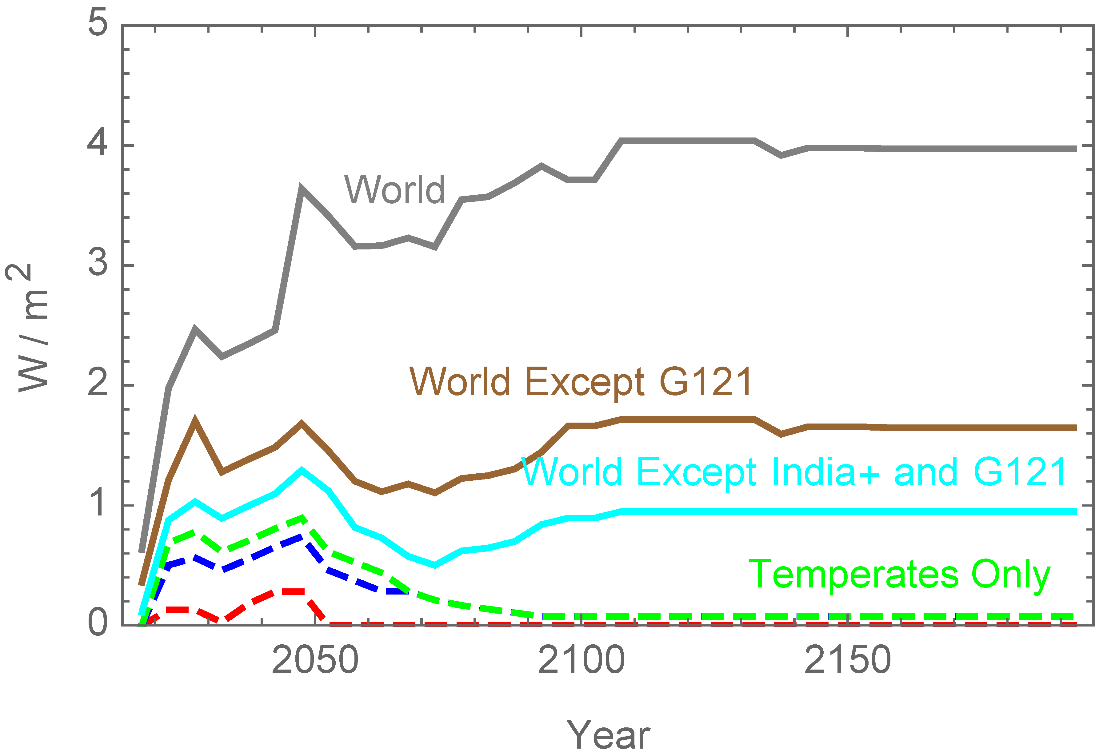
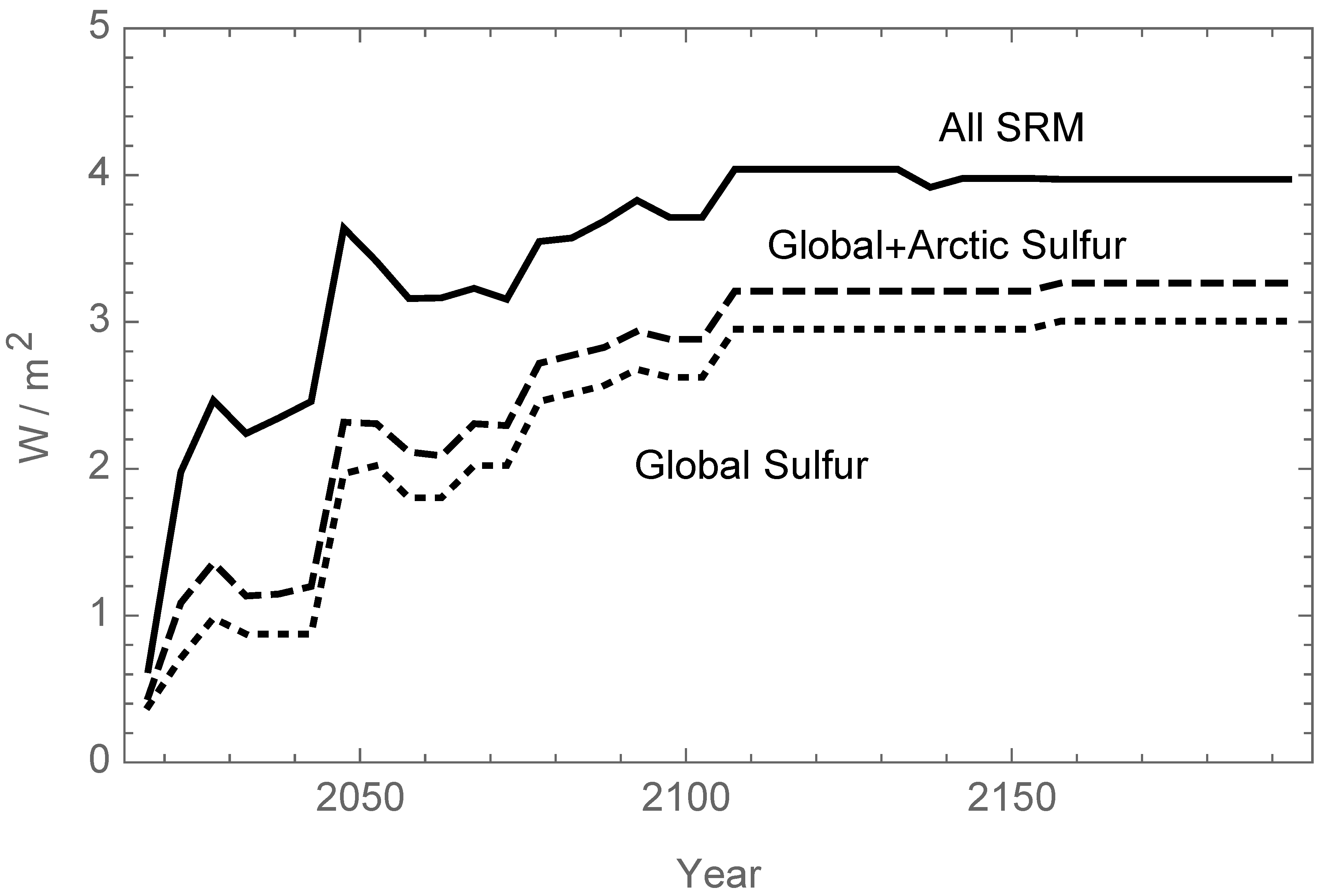
As shown in Figure 2, the atmospheric ${\text{CO}}_2$ concentration had nearly doubled its preindustrial 280 ppmv level by 2045, and it was continuing to rise due to a stabilized but still substantial rate of global emissions. It took an abrupt increase in solar radiation management (SRM) via global albedo increase from 2045–2050, shown in Figure 7, to convince temperate regions to decarbonize further. That increase in SRM was primarily implemented by the predominantly tropical and subtropical regions, Ocean, India+ and G121, as shown in Figure 6. That level of SRM reduced global average temperature as shown in Figure 2 to well below the optimum for the three more temperate regions as shown in Figure 5. This approach and the temperate region’s response of cooperating with lowering greenhouse gas emissions was the outcome of a set of extensive discussions amongst the simulation participants. This resulted in policies that caused global ${\text{CO}}_2$ emissions to drop after 2060. Temperature gradually recovered to 0.76 °C above preindustrial times, reflecting a compromise in between the optimum values for the temperate and more tropical regions.

Of the SRM methods available to participants, global stratospheric sulfur injection was the most popular choice (see Figure 7). This choice was modeled as incurring lower direct costs of implementation than the other two options, namely arctic stratospheric sulfur injection and low altitude salt water lofting (cf. Section 4.2). In this version of the simulation, global stratospheric sulfur injection was disabled for China+, the USA+ and the EU+ regions during the first six rounds of negotiation, because in previous simulations other participants in these regions had over-used global injection to the detriment of their own GDPs before fully understanding the consequences. Arctic stratospheric sulfur injection and low altitude seawater lofting were enabled and used on an exploratory basis from the outset by the temperature regions, with summed effect indicated by the dashed curves in Figure 6.

Figure 6. Solar radiation management by region. Included in curves from the lowermost upward are China+, USA+, EU+, Ocean, India+, and G121.

Figure 6. Solar radiation management by region. Included in curves from the lowermost upward are China+, USA+, EU+, Ocean, India+, and G121.

Figure 7. Global albedo modification for solar radiation management, by type.

Figure 7. Global albedo modification for solar radiation management, by type.

Final balances in trillions of U.S. dollars are listed in Table 2. (All dollar figures are inflation adjusted to year 2015 U.S. purchasing power parity.) Overall, at the end of the simulation, the global sum of pot balances was 461 trillion dollars, which represents 1.17 times the total extrapolated annual GDP in 2195.

Table 2. Example simulation pot balances in T$US2015.

Year	China+	USA+	EU+	Ocean	India+	G121
2045	4	4	3	8	5	6
2075	7	7	6	24	7	20
2105	12	12	8	46	29	30
2135	13	13	9	82	42	34
2165	12	12	11	151	65	28
2195	13	13	15	285	101	9

Table 2. Example simulation pot balances in T$US2015.

Year	China+	USA+	EU+	Ocean	India+	G121
2045	4	4	3	8	5	6
2075	7	7	6	24	7	20
2105	12	12	8	46	29	30
2135	13	13	9	82	42	34
2165	12	12	11	151	65	28
2195	13	13	15	285	101	9

The economic effects of the global average cooling mentioned above are reflected in Table 2. From 2045 to 2075, the temperature declined from 0.65 °C to 0.44 °C. The tropical countries experienced a consequent rise in pot balances. The G121 region postponed the cost of decarbonization of energy sources until it was able to afford reductions of ${\text{CO}}_2$ without ever having a negative pot balance. This outcome is qualitatively consistent with the assertions of some developing countries in modern climate negotiations that developing countries need to move forward with economic development without incurring large direct costs for limiting their greenhouse gas emissions.

2.7. Variations of the Climate Change Simulation Game

The simulation results described above were a product of the particular model described qualitatively Section 2.1, Section 2.2, Section 2.3, Section 2.4, Section 2.5 and quantitatively in Section 4. The Excel spreadsheets used to support that simulation allow for many possible modifications for purposes of education, research, and support of public policy formulation. For example, another simulation exercise used 60% of the energy decarbonization costs shown in Figure 3. This simulation had a qualitatively similar outcome to the one described here, but the final atmospheric ${\text{CO}}_2$ concentration dropped from 795 to 793 ppmv between 2190 and 2195. The participants in the simulation producing this result were different sets of undergraduate and graduate students. Only with a large number of randomized trials would it be possible to discern whether such difference in outcome are due to differences in the participant set or differences in the simulation parameters.

To add an element of randomness to the simulation, the Excel spreadsheet includes an ability to sample probability distributions to select model parameters. Conducting a large number of simulations using such probability distribution samples and sets of participants randomly selected from a sizeable pool would account for both differences between participants and uncertainty in parameters. The Excel spreadsheet also allows for simulation parameters to evolve over time through a Markov process. After each 30-year generation, samples from a log-normal probability distribution with mean 1.0 can multiply the then-current value of each selected parameter, with the variance of the probability distribution decreasing with each successive generation. While these probability distribution features are incorporated in the model for possible future use, running large numbers of simulations to explore the implications of uncertainties in model parameters is beyond the scope of the present work. Also, while the key parameters in the global heat and carbon balance models and the reference case GDP and energy and carbon use models were at calibrated against observational data (cf. [6] and references therein), these calibration exercises need to be updated and extended to calibrate probability distributions for model parameters. In particular, the parameters in the land ice model and most of the parameters in the financial model should be viewed as place holders pending a very extensive review of the literature to assign probability distributions to model parameters. That would be quite a complex task that could take years to accomplish; hence the report in the present work on results using the current state of the simulation model. It is to be emphasized that the purpose of the present paper is to illustrate the use of a methodology for investigating the feedback of effects of greenhouse gas emissions on policy responses, not to present a specific prediction of what that response is actually likely to be. That more ambitious goal would also require careful examination and control of how the selection of participants and instructions given to them affect the outcome, in order to see whether or not generic trends in outcomes emerge, or whether participants and moderators need to be chosen from amongst persons who are or are representative of or likely to become directly involved in relevant policymaking.

The simulation could also be expanded to more participants with regions being smaller groups of countries or single countries. In progress at the time of writing is calibration of demographics, GDP, and energy and carbon use for a set of 63 different regions, many of which consist of only one country. Groups of these countries and regions could be combined to support up to 63 participants per simulation.

The simulation has also been conducted with each participant being given a time limit for entering policy decisions and the Excel file being updated upon each entry via Google Drive. This, in principle, allows for participants who are geographically distributed and not otherwise in contact with each other. While this approach functions with a small number of participants, use of a dedicated server with faster response time may be necessary with substantially more than six participants.

The simulations performed so far have been in an exploratory mode, with each simulation conducted at least somewhat differently than the previous one. Some aspects of how the simulation implementation methods affect the results have nevertheless become apparent. First, the results of the simulation appear to be less erratic if the participants have previously accomplished a "queen or king of the world” exercise, where they individually chose all regions’ policies and try to achieve a globally optimal result. An interesting observation is that global end pot balances resulting from a subsequent interactive simulation have uniformly been substantially lower than the average achieved by each participant acting in "queen or king of the world” mode.

Each simulation has had a moderator, in some cases mostly passively just collecting policy decisions and entering them in the spreadsheet, and in other cases more actively providing input on the likely implications of policy choices and sometimes encouraging participants to talk with each other about upcoming policy decisions. It is not surprising that end global pot balance tends to be higher with an active and well informed moderator. This observation indicates the importance of choosing the moderator’s background and role carefully both during simulation exercise design and in real world global interactions on climate change policy.

Another observation from simulations done so far is that the choice of the percentage of total GDP for each region assigned to the regionâᾸŹs pot balance has a significant psychological effect on participants’ policy choices. Participants who have negative pot balances frequently report feeling “too poor” for more reduction in carbon emissions even if they represent regions with high per capita GDP. The importance of this psychological effect could be investigated by increasing the percentages of GDP assigned to pot balances and tasking participants with trying to maintain higher balances than participants in previous simulations, rather than trying to avoid negative balances.

3. Conclusions

The work described here provides an interesting starting point for experimental exploration of possibilities for future policy responses to expectations of results of climate change. Both the formulation of the model and experimental design require considerable additional work before being useful as quantitative tools for estimating probability distributions for actual future outcomes for climate change. Four sources of variability in the outcomes need to be investigated in such an exercise.

• The results will vary from one simulation to another even with different groups of participants selected at random from a pool of potential participants, even when given the same instructions and a model with the same input parameters and a moderator following the same set of instructions by rote.

• The results will be influenced by the instructions given to the participants and moderator.

• The results will be different on average for participants selected at random from different pools of potential participants.

• The results will be different if different sets of model parameters are selected from probability distributions for the parameters.

An exploration of all of these sources of variability would be a substantial but interesting exercise. A useful starting point could be to have potential researchers planning modeling exercises to themselves act as participants in simulations. However, even at the present stage the simulations have proven both to be a useful educational tool and to provide some qualitative insights into how solar radiation management might interact with policy constraints on net emissions of greenhouse gases.

4. Appendix on Computational Methods

4.1. Physical Balances

Atmospheric carbon content $c_a$ in trillions of metric tons (TtC) is related to atmospheric carbon dioxide concentration 〈${\mathrm{CO}}_2\rangle$ in pp1000v (parts per thousand by volume) by 〈${\mathrm{CO}}_2\rangle =c_4{c}_a$ where $c_4=1/2.13$. Atmospheric carbon content evolves according to the equation

$$\frac{d{c}_a}{dy}=\left(c_8+c_9\frac{c_a-c_5}{c_a+c_6{c}_5}+c_{10}\frac{\tau }{\tau +c_{11}}\right)E_c-\frac{c_a-c_5}{c_7}$$

(1)

Here y is time in years after Julian year 2000. The term containing the constant $c_9$ accounts for reduction of the fraction of anthropogenic ${\mathrm{CO}}_2$ emissions promptly moved into non-atmospheric reservoirs as 〈${\mathrm{CO}}_2\rangle$ increases. The term containing the constant $c_{10}$ accounts for the impact of increasing global average and surface ocean layer temperature on ${\mathrm{CO}}_2$ uptake in non-atmospheric reservoirs. Here $E_c$ is the global sum of a reference set of regional atmospheric carbon emissions that have each been multiplied by linearly interpolated values of factors $(1-f_c)$ determined from participants’ inputs as discussed above. Over a wide range of conditions, the solutions of this equation reproduce well within modeling uncertainties the results from the more complex four-chamber global carbon balance used by Singer et al. [5,17,33]. Each region has a maximum rate of carbon biosequestration that is based on its forestry potential. Each participant specifies her or his fraction of this maximum as an input value $G_{\mathrm{bio}}$.

Table 3 lists reference values of parameters common to all regions. It is to be emphasized that the reference parameter values listed in this appendix are not all meant to be the most likely values appropriate to simulating the future evolution and effects of climate change. Rather, particularly for costing model reference parameters listed in Section 4.2, values are chosen to illustrate points of particular educational interest. It is up to other users of the type of spreadsheets described here to insert parameter values appropriate to their particular interests.

The evolution of arctic land ice volume v, divided by its starting value at $y=15$, is given by

$$dv/dy=-(1-c_{13}{G}_{\mathrm{artic}})(c_{14}-v)\tau /c_{15}$$

(2)

for $v>0$ (with $dv/dy=0$ when $v=0$ so that v does not become negative). $G_{\mathrm{artic}}$ is the sum of regional input values as used in the line after Equation (5) below, but at most 100% = 1 if those inputs sum to more than 100%. The constant $c_{13}$ is a measure of the summer to annually averaged global effect of arctic stratospheric sulfur injection, which is more than the ratio of the incident sunlight per unit area times the surface area of the whole globe to that for the arctic, i.e., a large number. For the example described above, the differential effect of arctic vs. global stratospheric sulfur injection had not yet been implemented in the model, so that exercise in effect had $c_{13}=0$. Thus, in the exercise described above, the effect of using arctic instead of global stratospheric sulfur injection is just to avoid the direct negative economic effects of a global stratospheric haze that are described below. Here τ is the increase in global average temperature over a pre-industrial reference level. The inclusion of the factor $(c_{14}-v)$ accounts for the temperature on the surface of the Greenland ice sheet increasing as its altitude decreases as a result of accumulated melting, in addition to the melting proceeding faster for larger values of τ. For the results presented here, $c_{14}=2$.

Table 3. Physical parameters.

Symbol	Value	Units	Meaning
c4	1/2.13	pp1000v/TtC	Conversion factor
c5	0.5964	TtC	Preindustrial average
c6	0.5	1	Ocean saturation parameter
c7	1350	yr	Timescale for CO2 sinking to deep ocean
c8	0.48	1	Preindustrial fraction of CO2 retained in atmosphere
c9	0.40	1	Maximum non-atmospheric CO2 saturation effect
c10	0.12	1	Maximum thermal effect on atmospheric CO2 retention
c11	3	°K	Temperature for half maximum thermal effect on CO2 retention
c13	1	1	Differential effect of arctic sulfur on ice melting
c14	2	1	Ice altitude effect parameter
c15	4000	years	Arctic land ice melting timescale parameter
c17	30.667	(W/m2)°K/yr	Ocean surface layer thermal inertia parameter
c18	341.5	(W/m2)	Surface- and time-average reference insolation
c19	286.85	°K	Time-averaged preindustrial global average temperature
c20	1.16	1	c20-c22 is the preindustrial average albedo
c21	0.87	1	c21-c23 is the preindustrial effective emissivity
c22	0.86055	1	Ice albedo parameter
c23	0.24685	1	Temperature effect on effective emissivity
c26	0.0002	1	Insolation fractional increase at Gleisburg cycle maximum
c27	0.0004	1	Insolation fractional increase at long sunspot cycle maximum
c28	–3	years	Time of Gleisburg cycle maximum, measured from year 2000
c29	–3	years	Time of long period sunspot cycle maximum, "
c30	88	yr	Gleisburg cycle period
c31	600	yr	Long sunspot cycle period
c40	0.0160	1	Maximum global sulfur fractional effect on net insolation
c41	0.0038	1	Maximum arctic sulfur fractional effect on net global insolation
c42	0.0090	1	Maximum saltwater lofting effect on net global insolation
c55	7.66	m	Sea level rise from all northern hemisphere land ice
c57	0.031462	m/°K	Linear term thermal expansion coefficient
c58	0.000138	m/(°K)2	Quadratic term thermal expansion coefficient

Table 3. Physical parameters.

Symbol	Value	Units	Meaning
c4	1/2.13	pp1000v/TtC	Conversion factor
c5	0.5964	TtC	Preindustrial average
c6	0.5	1	Ocean saturation parameter
c7	1350	yr	Timescale for CO2 sinking to deep ocean
c8	0.48	1	Preindustrial fraction of CO2 retained in atmosphere
c9	0.40	1	Maximum non-atmospheric CO2 saturation effect
c10	0.12	1	Maximum thermal effect on atmospheric CO2 retention
c11	3	°K	Temperature for half maximum thermal effect on CO2 retention
c13	1	1	Differential effect of arctic sulfur on ice melting
c14	2	1	Ice altitude effect parameter
c15	4000	years	Arctic land ice melting timescale parameter
c17	30.667	(W/m2)°K/yr	Ocean surface layer thermal inertia parameter
c18	341.5	(W/m2)	Surface- and time-average reference insolation
c19	286.85	°K	Time-averaged preindustrial global average temperature
c20	1.16	1	c20-c22 is the preindustrial average albedo
c21	0.87	1	c21-c23 is the preindustrial effective emissivity
c22	0.86055	1	Ice albedo parameter
c23	0.24685	1	Temperature effect on effective emissivity
c26	0.0002	1	Insolation fractional increase at Gleisburg cycle maximum
c27	0.0004	1	Insolation fractional increase at long sunspot cycle maximum
c28	–3	years	Time of Gleisburg cycle maximum, measured from year 2000
c29	–3	years	Time of long period sunspot cycle maximum, "
c30	88	yr	Gleisburg cycle period
c31	600	yr	Long sunspot cycle period
c40	0.0160	1	Maximum global sulfur fractional effect on net insolation
c41	0.0038	1	Maximum arctic sulfur fractional effect on net global insolation
c42	0.0090	1	Maximum saltwater lofting effect on net global insolation
c55	7.66	m	Sea level rise from all northern hemisphere land ice
c57	0.031462	m/°K	Linear term thermal expansion coefficient
c58	0.000138	m/(°K)2	Quadratic term thermal expansion coefficient

The increase in global mean sea level, M in meters, over its year 2015 accounts for land ice melting and thermal expansion of the surface ocean layer as the global average temperature changes from its year 2015 value of $T_1=T_0$ + 0.785 °C.

$$M=c_{55}(1-v)+c_{57}(T-T_1)+c_{58}{(T-T_1)}^2$$

(3)

Global average temperature evolves as

$$c_{17}\frac{d\tau }{dy}=c_{18}(\mu -G)(1-c_{20}+c_{22}{(T/T_0)}^2)-c_{24}{(1+\tau /T_0)}^4(c_{21}-c_{23}{(T/T_0)}^2-F)$$

(4)

Here $\tau =T-T_0=T-c_{19}$ is the change in global average temperature T from a preindustrial reference value of $c_{19}=286.85°K$. Also, $c_{24}=\sigma T_0^4$, where $\sigma =5.6704\times {10}^{-8}$ W/(m²² °K⁴) is the Stefan-Boltzmann constant. The term $c_{22}{(T/T_0)}^2$ is included to account for the “ice-albedo” effect; higher temperature leads to lower global average snow and ice cover and thus decreases reflection of incident sunlight. The term $c_{23}{(T/T_0)}^2$ accounts for the greenhouse effect of atmospheric water vapor net of changes in cloud cover. This simple approach to inclusion of these effects is derived from an early paper by Fraedrich [32] and was calibrated against more recent data by Milligan [33], as was the reference surface ocean thermal inertia timescale of $c_{17}$ = 30.667 (W/m²)(yr/°K). The factor μ includes small sinusoidal variations with periods of 88 and 600 years affecting the solar insolation with surface averaged reference value $c_{18}=(1366/4)$ W/m². The effects of the short-period variable 11-year sunspot cycles are assumed to average out, so those periodic variations in insolation are not included. The formula for μ is

$$\mu =1+c_{26}\mathrm{Cos}[2\pi (y-c_{28})/c_{30}]+c_{27}\mathrm{Cos}[2\pi (y-c_{29})/c_{31}]$$

(5)

The global effect of solar radiation management is given by the sum $G=c_{40}{G}_{\mathrm{sulfur}}+c_{41}{G}_{\mathrm{arctic}}+c_{42}{G}_{\mathrm{salt}}$ of the effects of global coverage stratospheric sulfur injection $G_{\mathrm{sulfur}}$, seasonal arctic stratospheric sulfur injection $G_{\mathrm{arctic}}$, and low-altitude salt water lofting $G_{\mathrm{salt}}$. The costs associated with the components of G are described in Section 4.2. The radiative forcing effect of increases in atmospheric greenhouse gas concentrations over reference levels is given by the sum $F=F_C+c_{38}(F_F+F_N)$ of effects of ${\mathrm{CO}}_2$, volatile fluorine compounds, and ${\text{N}}_2$O. The formula for $F_C$ is $F_C=c_{33}\mathrm{Ln}[c_a/c_5]$, where the reference value used for the results presented here is $c_{33}=0.0068$.

The formula for the effect of nitrous oxide on global average temperature is

$$F_N=c_{52}(\sqrt{N}-{\sqrt{c}}_{44})-(F_{MN}-c_{45})$$

(6)

where

$$F_{MN}=c_{46}\mathrm{Ln}[1+c_{48}{(c_{47}N)}^{c_{50}}+c_{49}{(c_{47}N)}^{c_{51}}]$$

(7)

Here $c_{44}=270$ is the preindustrial atmospheric ${\text{N}}_2$O concentration in parts per billion by volume (ppbv). The factor $F_{MN}$ accounts for overlapping methane and nitrous oxide absorption bands [29]. The constant $c_{47}=1803$ is a recent reference value for the atmospheric methane concentration in ppbv. The result from this formula for $F_N$ is less than that from a simple linear function $0.00315(N-c_{44})$ by only 0.4 percent for $N=329$ ppbv but by 12 percent for the no-reductions result of $N=506$ ppbv for year 2195. Reference values of parameters in the ${\text{N}}_2$O balance model are listed in Table 4.

The effect of future changes in the atmospheric methane concentration is not accounted for here. This is because the rate of methane emissions has recently nearly stabilized and methane has a short atmospheric lifetime compared to the time scales of primary interest here. If there are nevertheless substantial future increases in the atmospheric methane concentration, it is assumed here that the resulting radiative forcing will be cancelled by global albedo increase at a cost that is insubstantial compared to that for reducing radiative forcing from other greenhouse gases.

Table 4. Global nitrous oxide parameters.

Symbol	Value	Units	Meaning
$c_{38}$	0.00126	yr	Minor greenhouse gas forcing effect coefficient
$c_{43}$	5	yr	Times over which N2O emissions are held constant
$c_{44}$	270	ppbv	Preindustrial atmospheric N2O concentration
$c_{45}$	0.149	ppbv	Preindustrial $<{\mathrm{CH}}_4>$ correction to N2O forcing
$c_{46}$	0.47	W/m2	Coefficient for $<{\mathrm{CH}}_4>$ correction to N2O forcing
$c_{47}$	1803	ppbv	$<{\mathrm{CH}}_4>$ for correction to N2O forcing
$c_{48}$	$2.01\times {10}^{-5}$	${\mathrm{ppbv}}^{-2c_{50}}$	Coefficient for $<{\mathrm{CH}}_4>$ correction to N2O forcing
$c_{49}$	$1.52\times {10}^{-15}$	${\mathrm{ppbv}}^{-2c_{51}}$	Coefficient for $<{\mathrm{CH}}_4>$ correction to N2O forcing
$c_{50}$	0.75	1	Exponent for $<{\mathrm{CH}}_4>$ correction to N2O forcing
$c_{51}$	1.52	1	Exponent for $<{\mathrm{CH}}_4>$ correction to N2O forcing
$c_{52}$	0.12	(W/m2)/$\sqrt{\mathrm{ppbv}}$	Coefficient for N2O forcing
$c_{53}$	121	yr	Inverse of excess atmospheric N2O clearing rate

Table 4. Global nitrous oxide parameters.

Symbol	Value	Units	Meaning
$c_{38}$	0.00126	yr	Minor greenhouse gas forcing effect coefficient
$c_{43}$	5	yr	Times over which N2O emissions are held constant
$c_{44}$	270	ppbv	Preindustrial atmospheric N2O concentration
$c_{45}$	0.149	ppbv	Preindustrial $<{\mathrm{CH}}_4>$ correction to N2O forcing
$c_{46}$	0.47	W/m2	Coefficient for $<{\mathrm{CH}}_4>$ correction to N2O forcing
$c_{47}$	1803	ppbv	$<{\mathrm{CH}}_4>$ for correction to N2O forcing
$c_{48}$	$2.01\times {10}^{-5}$	${\mathrm{ppbv}}^{-2c_{50}}$	Coefficient for $<{\mathrm{CH}}_4>$ correction to N2O forcing
$c_{49}$	$1.52\times {10}^{-15}$	${\mathrm{ppbv}}^{-2c_{51}}$	Coefficient for $<{\mathrm{CH}}_4>$ correction to N2O forcing
$c_{50}$	0.75	1	Exponent for $<{\mathrm{CH}}_4>$ correction to N2O forcing
$c_{51}$	1.52	1	Exponent for $<{\mathrm{CH}}_4>$ correction to N2O forcing
$c_{52}$	0.12	(W/m2)/$\sqrt{\mathrm{ppbv}}$	Coefficient for N2O forcing
$c_{53}$	121	yr	Inverse of excess atmospheric N2O clearing rate

Also,

$$F_F={\Sigma }_{k=1}^{10}{F}_k$$

(8)

where $F_k=b_{4,k}{A}_k$ for $k=1\dots 10$, and $A_k$ are the atmospheric contents in ktonne of ten volatile fluorine compounds. Here $b_{4,k}$ are the forcing coefficients listed in the fourth column of Table 5, multiplied by $c_4{A}_C/M_k$ where $(c_4/1000)A_C/M_k$, with $c_4=1/2.13$, $A_C=12.0107$ is the atomic weight of carbon, and $M_k$ are the molecular weights listed in Table 5. The factors $c_4{A}_C/M_k$ convert total ktonne of each fluorine compound in the atmosphere to parts per trillion by volume (pptv). The values of $A_k$ evolve as

$$d{A}_k/dt=E_k-A_k/b_{5,k}$$

(9)

where $E_k$ are global emissions rates and $b_{5,1}\dots b_{5,10}$ are the atmospheric lifetimes listed in the third column in Table 5. The starting values for $A_k$ at $y=15$ are listed in Table 5. Reference values for the other parameters pertinent to volatile fluorine compounds are also listed in Table 5.

Global emissions based on logistic fits to IPCC scenario A2 extrapolations [2] are divided in proportion to each region’s GDP in order to estimate the values of $E_{0k}$ as functions of time. The year 2100 A2 scenario value for HFC43-10 was multiplied by 3/4 to make it similar to the other fits instead of having a half-maximum in Julian year 2364. The logistic fits are of the form

$$b_{k,1}/(1+e^{-(y-b_{k,2})/b_{k,3}})\mathrm{for}k=1\dots 10$$

(10)

Atmospheric nitrous oxide concentration N evolves as the solution to the equation

$$dN/dt=S-(N-c_{44})/c_{53}$$

(11)

with the initial condition $N=327.6$ ppbv at $t=2015$. Here $c_{52}=121$ years. The source term is $S={\sum }_{n=1}^6{S}_n$ with $S_n=(1-r_n)f_{n}G$ where $f_n$ is the fraction of global anthropogenic nitrous oxide emissions in reference year 2011 for region n. In the absence of reductions (i.e., if all $r_n$ = 0), G is $G=PL$ where $P={\sum }_{n=1}^6{P}_n$, and $P_n=p_{0n}+p_{1n}/(1+\mathrm{Exp}[(p_{2n}-t)/p_{3n}])-Q_n$ with $t=2000+y$ and the values of the constants listed in Table 6, and $Q_n=p_{0n}+p_{1n}/(1+\mathrm{Exp}[-(p_{2n}-1860)/p_{3n}])$. The logistic function $L=4.81(0.6236+0.3571/(1+\mathrm{Exp}[-(1968.05-t)/2.701])$ accounts for an increase the incremental nitrogen in nitrous oxide emissions over 1860 values per incremental population increasing from about 0.62 (kg/yr)/person before widespread use of manufactured nitrogen fertilizer to about 0.98 (kg/yr)/person thereafter. The leading coefficient of 4.81 converts Mtonne (10⁹ kg) of atmospheric nitrogen in nitrous oxide to ppbv of N₂O.

Table 5. Parameters for volatile fluorine compounds.

HFC	Chemical	Life	Force	mol wt	Initial	b1	b2	b3
Code	Formula	(yr)	(W/m2)/ppbv	gm/mol	kt	kt/yr	yr	yr
HFC32	CH2F2	5.6	0.11	52.02	5.34	48.6	77.6	30.6
HFC43-10	CF3CF2(CHF)2CF3	17.1	0.40	141.09	0.21	26.4	71.9	57.4
HFC125	CHF2CF3	32.6	0.23	82.02	10.47	155.4	76.5	30.2
HFC134a	CH2CF3	14.6	0.16	83.03	64.70	2625.8	103.0	37.0
HFC143	CH3CF3	48.3	0.13	62.03	12.87	120.8	77.1	30.4
HFC227ea	CH3CHFCF3	36.5	0.26	114.04	0.53	266.8	135.9	42.7
HFC245ca	CH2F2 CH2CF3	6.6	0.21	134.05	2.16	1493.8	145.5	43.4
	CF4	10000	0.10	88.00	80.04	131.7	73.6	37.2
	C2F6	2600	0.26	138.01	4.23	12.5	69.1	35.5
	SF6	3200	0.52	146.60	7.52	30.8	47.3	35.1

Table 5. Parameters for volatile fluorine compounds.

HFC	Chemical	Life	Force	mol wt	Initial	b1	b2	b3
Code	Formula	(yr)	(W/m2)/ppbv	gm/mol	kt	kt/yr	yr	yr
HFC32	CH2F2	5.6	0.11	52.02	5.34	48.6	77.6	30.6
HFC43-10	CF3CF2(CHF)2CF3	17.1	0.40	141.09	0.21	26.4	71.9	57.4
HFC125	CHF2CF3	32.6	0.23	82.02	10.47	155.4	76.5	30.2
HFC134a	CH2CF3	14.6	0.16	83.03	64.70	2625.8	103.0	37.0
HFC143	CH3CF3	48.3	0.13	62.03	12.87	120.8	77.1	30.4
HFC227ea	CH3CHFCF3	36.5	0.26	114.04	0.53	266.8	135.9	42.7
HFC245ca	CH2F2 CH2CF3	6.6	0.21	134.05	2.16	1493.8	145.5	43.4
	CF4	10000	0.10	88.00	80.04	131.7	73.6	37.2
	C2F6	2600	0.26	138.01	4.23	12.5	69.1	35.5
	SF6	3200	0.52	146.60	7.52	30.8	47.3	35.1

Table 6. Region dependent nitrous oxide parameters.

Symbol	Units	China+	USA+	EU+	Ocean	India+	G121
$p_0$	Gpersons	0.388	0.011	0.231	0.080	0.224	0.114
$p_1$	Gpersons	1.525	0.593	0.827	1.073	2.801	4.974
$p_2$	Julian year	1965.76	1993.23	1936.01	1979.40	1999.04	2028.10
$p_3$	Years	19.14	48.62	19.90	28.27	28.97	33.11
f	1	0.142	0.204	0.169	0.204	0.117	0.163

Table 6. Region dependent nitrous oxide parameters.

Symbol	Units	China+	USA+	EU+	Ocean	India+	G121
$p_0$	Gpersons	0.388	0.011	0.231	0.080	0.224	0.114
$p_1$	Gpersons	1.525	0.593	0.827	1.073	2.801	4.974
$p_2$	Julian year	1965.76	1993.23	1936.01	1979.40	1999.04	2028.10
$p_3$	Years	19.14	48.62	19.90	28.27	28.97	33.11
f	1	0.142	0.204	0.169	0.204	0.117	0.163

The above differential equations for $c_a$, τ, v and N are solved using a simple Euler method with a time step equal to $\delta =2.5$ years. That is, equations of the form $dX/dt=R$ are advanced by setting $X_{j+1}=X_j+R_j\delta$, where $R_j$ is evaluated using results from time $y_j$, where $y_j=12.5+j$ for as many values of j as desired. Values for even numbers j are taken to approximate averages over five year periods for the purpose of estimating changes in pot balances. Exact analytic solutions for atmospheric contents of volatile fluorine compounds are used, with emissions $E_k$ approximated as constant averages in each 5-year period between initial and final emission levels over the 5-year period as specified by participants’ inputs.

4.2. Costing

Each parameter in the costing model has a spreadsheet representation as a scalar times a vector with number of components equal to the number of regions. Here these products are denoted by a letter d with a subscript. Reference values of these parameters listed in Table 7 are the same for all regions, except for the greater sensitivity of the Ocean and India+ regions to incremental sea level rise due to melting of arctic land ice as indicated in Table 1. However, the spreadsheet includes options for making any or all of these parameters different for different regions.

Table 7. Global financial parameters.

Symbol	Value	Units	Meaning
$d_4$	0.0006	1	Parameter for fraction of GDP loss from direct 〈CO2〉 effect
$d_5$	0.0004	1	Minimum fraction of GDP loss from artic land ice melting (cf. Table 1)
$d_9$	10	(yr/°K)2	Parameter for fraction of GDP loss proportional to ${(d\tau /dy)}^2$
$d_{10}$	0.05	T$/GtC	Initial cost of energy decarbonization
$d_{11}$	3	1	Coefficient of cost of changing carbonization vs. $|f_c|$
$d_{12}$	4	1	Exponent for cost of changing carbonization vs. $|f_c|$
$d_{13}$	3	1	Limiting parameter for cost of decarbonization
$d_{14}$	0.4	T$(yr/GtC)	Annual cost proportional to rate of change of carbon emission
$d_{15}$	0.1	T$/GtC	Cost of carbon biosequestration
$d_{17}$	6.9	T$	Annual cost per fraction of maximum stratospheric injection
$d_{18}$	0.02	1	% of GDP lost per % of maximum global stratospheric sulfur
$d_{19}$	7.5	T$	Annual cost per fraction of maximum arctic sulfur injection
$d_{21}$	16.2	T$	Annual cost per fraction of maximum saltwater lofting
$d_{23}$	2.3	%	Annual interest rate on pot balances
$d_{25}$	1	°K	Reference temperature in warming damage functions
$d_{26}$	2	1	Multiplier for warming cost damage functions
$d_{42}$	2.9773	T$/ppbv	Coefficient of cost of N2O reductions
$d_{43}$	1	1	Coefficient for cost of biosequestration

Table 7. Global financial parameters.

Symbol	Value	Units	Meaning
$d_4$	0.0006	1	Parameter for fraction of GDP loss from direct 〈CO2〉 effect
$d_5$	0.0004	1	Minimum fraction of GDP loss from artic land ice melting (cf. Table 1)
$d_9$	10	(yr/°K)2	Parameter for fraction of GDP loss proportional to ${(d\tau /dy)}^2$
$d_{10}$	0.05	T$/GtC	Initial cost of energy decarbonization
$d_{11}$	3	1	Coefficient of cost of changing carbonization vs. $|f_c|$
$d_{12}$	4	1	Exponent for cost of changing carbonization vs. $|f_c|$
$d_{13}$	3	1	Limiting parameter for cost of decarbonization
$d_{14}$	0.4	T$(yr/GtC)	Annual cost proportional to rate of change of carbon emission
$d_{15}$	0.1	T$/GtC	Cost of carbon biosequestration
$d_{17}$	6.9	T$	Annual cost per fraction of maximum stratospheric injection
$d_{18}$	0.02	1	% of GDP lost per % of maximum global stratospheric sulfur
$d_{19}$	7.5	T$	Annual cost per fraction of maximum arctic sulfur injection
$d_{21}$	16.2	T$	Annual cost per fraction of maximum saltwater lofting
$d_{23}$	2.3	%	Annual interest rate on pot balances
$d_{25}$	1	°K	Reference temperature in warming damage functions
$d_{26}$	2	1	Multiplier for warming cost damage functions
$d_{42}$	2.9773	T$/ppbv	Coefficient of cost of N2O reductions
$d_{43}$	1	1	Coefficient for cost of biosequestration

The fraction of GDP lost due to direct effects of 〈${\mathrm{CO}}_2\rangle$ buildup is determined by $d_4{((ca/c_5)-1)}^2$. (Herein, GDP means annual gross domestic product.) The fractional change in GDP that is added (algebraically) to pot balances as a result of changes in arctic land ice volume is $-d_5(1-v)$ times the relative sea level rise cost multiplier listed in Table 1.

Some of the financial parameters are different for each region. For example, the fractional change in GDP as a function of τ that is added to pot balances is

$$d_{26}\left(\frac{1}{1+d_6(\tau -d_{25})+d_7{(\tau -d_{25})}^2}-1-0.001d_8\right)$$

(12)

Reference values of some parameters that are different for more than one region are listed in Table 8. Example results for such functions are plotted as percentages in Figure 5. These values are adapted from examples from Nordhaus and Boyer [30] as reported by Bosello and Roson [31]. Added to each pot balance also is the fractional change in GDP that depends on the rate of change of τ and is equal to $-d_9{(d\tau /dy)}^2$.

Table 8. Region dependent financial parameters.

Symbol	Units	China+	USA+	EU+	Ocean	India+	G121
$d_6$	1	–0.0041	–0.0042	–0.0050	0.0039	0.0050	0.0022
$d_7$	1	0.0020	0.0025	0.0049	0.0013	0.0049	0.0026
$d_8$	1	0.84082	0.83724	0.8941	–0.96895	–1.41385	–0.6234
$d_{16}$	GtC/yr	0.1100	0.2225	0.1300	0.2235	0.0320	0.7770
$d_{24}$	%	1.12	0.840	0.76	1. 42	1.24	1.02

Table 8. Region dependent financial parameters.

Symbol	Units	China+	USA+	EU+	Ocean	India+	G121
$d_6$	1	–0.0041	–0.0042	–0.0050	0.0039	0.0050	0.0022
$d_7$	1	0.0020	0.0025	0.0049	0.0013	0.0049	0.0026
$d_8$	1	0.84082	0.83724	0.8941	–0.96895	–1.41385	–0.6234
$d_{16}$	GtC/yr	0.1100	0.2225	0.1300	0.2235	0.0320	0.7770
$d_{24}$	%	1.12	0.840	0.76	1. 42	1.24	1.02

The direct change in pot balance for reduction of annual atmospheric carbon emissions for a region is given by

$$-d_{10}(1+\mathrm{Min}[d_{13},d_{11}{f}_c^{d12}])f_c{E}_{c0}$$

(13)

where $E_{c0}$ is the region’s no additional policy carbon emissions rate. For the results shown here, $d_{13}=d_{11}=3$ and $d_{12}=4$. The marginal cost per metric ton of energy decarbonization that that gives this average cost is $d_{10}(1+15f_c^4)$. For the reference example results shown above, $d_{10}$ = 50$/tC, giving a marginal cost of $143/tC for $f_c=0.58$. In 2010, Enkvist et al. [38] estimated a marginal cost from new coal carbon and sequestration plants at $f_c=0.58$ of about 40 euro/tCO₂ by 2030, which corresponds to $200/tC in the monetary units used here. However, these authors estimate a zero marginal cost at about $f_c=0.21$, so their average cost at $f_c=0.58$ is lower than what would result from the formula used here with $d_{10}$=(200/143)50$/tC. In the approach used here, the marginal cost of decarbonization is always positive. This approach reflects an assumption that large scale energy decarbonization up to a point of zero marginal cost continues to be precluded by system inefficiencies (such as non-nuclear renewable energy mandates being used instead of across the board carbon emission taxes).

The annual change in pot balances due to each region changing its emissions rate with time is given by $-d_{14}\mathrm{Max}[0,d(f_c{E}_{c0})/dy]$. With this formula included, regions can avoid extra costs by avoiding rapid buildup of carbon-intensive energy systems, which is primarily a consideration for the China+ region. To account for the costs of decommissioning carbon-intensive energy systems before the end of their otherwise normal operating lifetimes, this formula should be modified to include costs for very rapid energy decarbonization.

The formula $-d_{15}(1+d_{43}{f}_{\mathrm{bio}}/2)$ gives the annual T$US2015 change in pot balances per Gtonne of carbon annually biosequestered. This formula results from assuming that the marginal cost per unit annual amount of carbon biosequestration increases linearly with the rate of biosequestration. The maximum annual rates of biosequestration are given by $d_{16}$.

The annual direct cost in T$US2015 to a region via global stratospheric sulfur injection is

$$d_{17}{c}_{40}{f}_{\mathrm{volcano}}{f}_{\mathrm{S}}$$

(14)

For $f_{\mathrm{volcano}}=1$, where $f_{\mathrm{volcano}}$ is defined below. For$f_{\mathrm{volcano}}=1$, this cost corresponds to a cost in T$US2015 per W/m² of radiative forcing of $d_{17}/c_{18}=0.02$. Klepper and Resnick [25] refers to a range of 0.002 to 0.012 T$ per W/m² for global sulfur (with references from 2008 to 2010 with no stated inflation adjustment.) To the extent that the range quoted in this reference is well reasoned, simulation participants have not been misled into adopting modest levels of stratospheric sulfur injection just because its direct cost was substantially underestimated. However, it should be noted a recent estimate of the radiative forcing in W/m² as a function of the global stratospheric sulfur injection rate X in Mtonne/yr is

$$-65e^{{(-2248/X)}^{0.23}}$$

(15)

so a radiative forcing of –6 W/m² requires five times the sulfur injection rate as does a radiative forcing of –6 W/m² [28]. Even so, global stratsopheric sulfur injection has comparatively low direct cost compared to extensive energy decarbonization, but the costing model used here should be modified in future work to account for the nonlinear response of radiative forcing to sulfur injection. The participants’ policy entries for stratospheric sulfur injection are linearly interpolated between an entry for year $y_j$ and $y_{j+1}$ to get a costing value used for time midway between $y_j$ and $y_{j+1}$. For example, a 1% decrease in $c_{18}(1-c_{20}+c_{22}{(T/T_0)}^2)$ costs 1% of $d_{17}$ T$/yr. The fractional change in each region’s GDP due to the globally summed rate thereof is $d_{18}$ times the summed value of the global coverage stratospheric sulfur injection entries in the participants’ spreadsheets. If the sum of all regions’ reductions in net insolation is greater than $d_{27}$, then each region’s entered value is multiplied by $d_{27}$ divided by that sum. Setting $d_{27}=0$ creates a simpler version for which entries for stratospheric sulfur injection has no effect.

The factor $f_{\mathrm{volcano}}$ is set equal to 1 for every quinquennium during which there is no significant insertion of sulfur into the stratosphere due to volcanic eruptions. If the effect of volcanic eruptions on the global heat balance averaged over a quinquennium is equal to or larger than that due to the sum of participants’ choices, then the cost to those participants is set to zero by setting $f_{\mathrm{volcano}}=0$ for each participant for that quinquennium (cf. [39]). If the effect of volcanic eruptions on the global heat balance is non-negligible but less than the global sum of participants decisions for stratospheric sulfur injection, then $f_{\mathrm{volcano}}$ is set equal to the ratio of the effect of volcanic eruptions to the sum of participants’ decisions for stratospheric sulfur. Volcanic eruptions have no effect on the global heat balance even if $f_{\mathrm{volcano}}>0$, since it is assumed that in such cases reductions in anthropogenic global stratospheric sulfur emissions over a five year period are equal to the increase in natural global stratospheric sulfur injection. Arctic volcanoes are assumed to have so little long term effect on land ice melting that only their effects on the global heat balance and thus on costs of global stratospheric sulfur injection costs are accounted for. Table 9 lists parameters from two examples of random samples from a stochastic model of future volcanic eruptions by Amman and Naveau [40]. For most purposes it suffices to choose one of these two examples but not inform participants ahead of time which is being used. If this is thought insufficient, simulation managers could use the method described by Amman and Naveau.

The changes in pot balances per unit increase in G in the heat balance equation for each region using seasonal arctic stratospheric sulfur injection are given by $-d_{19}$. If the sum of all regions’ reductions in net insolation is greater than 1, then each region’s entered value is divided by that sum. The changes in pot balances per W/m² reduction for each region using low-altitude salt water lofting are given by $-d_{21}$. If the sum of all region’s reductions in net insolation is greater than 1, then each region’s entered value is multiplied by $d_{22}$ divided by that sum.

Table 9. Two volcanic radiative forcing options.

Step	W yr/m2	Step	W yr/m2
6	2.08	9	1.76
8	3.88	15	0.21
9	0.92	24	0.77
10	1.40	30	1.20
11	2.32	32	8.48
12	2.42	36	1.20
21	0.29
27	3.53
29	0.43
31	1.98
35	0.77

Table 9. Two volcanic radiative forcing options.

Step	W yr/m2	Step	W yr/m2
6	2.08	9	1.76
8	3.88	15	0.21
9	0.92	24	0.77
10	1.40	30	1.20
11	2.32	32	8.48
12	2.42	36	1.20
21	0.29
27	3.53
29	0.43
31	1.98
35	0.77

The costs in T$US2015/year per annual ktonne change in the absolute value $|E_{0k}-E_k|$ in emitted volatile fluorine compound of type k is $d_{k+30}|E_{0k}-E_k|$. Note that the use of absolute value in the formulas $d_{k+30}|E_{0k}-E_k|$ allows for the possibility of increasing emission of volatile fluorine compounds over their “no policy” emissions levels. These compounds are divided into three classes: refrigerants only, compounds with very long atmospheric half lives (SF₆, NF₃, and C₂F₆), and others (which include HFC43-10 and HCC 227ea). By far the largest component of the “other” category is HFC134a (i.e., CH₂FCF₃). HFC134a is used both as a foam blowing agent and a refrigerant and has an atmospheric lifetime of 14 years. By increasing production and release the “other” category temporarily, regions wanting a higher global average temperature have the option of sending a signal to other regions that those other regions need to limit their rates of stratospheric sulfur injection.

Added annually to each region’s pot balance to help pay for various costs is $d_{24}$ times that region’s annual GDP. The annualized interest rate for earnings on positive balances and payments on negative balances are denoted as $d_{23}$.

The reference values of the parameters $d_{31}\dots d_{40}$ in the costing model for reducing emissions of volatile fluorine compounds are respectively 0.0001{3, 1, 3, 1, 3, 1, 3, 2, 2, 2} T$US2015/yr. The cost of reducing nitrous oxide emissions in region n by a fraction $r_n$ is $d_{42}{r}_n^2{f}_n{R}_n$, where $R_n$ is the ratio of “no new policy” N₂O emissions from region n at time $t=2015$ to the emissions from region n in 2015, and the values of $f_n$ are listed in Table 6.

References

- McNutt, M.K.; Abdalati, W.; Caldeira, K.; Coney, S.C.; Falkowski, P.G.; Fetter, S.; Fleming, J.R.; Hamburg, S.P.; Morgan, M.G.; Penner, J.E.; et al. Climate Intervention: Reflecting Sunlight to Cool Earth; National Academy of Sciences: Washington, DC, USA, 2015. [Google Scholar]
- Stocker, T.F., Qin, D., Plattner, G.-K., Tignor, M., Allen, S.K., Boschung, A., Nauels, A., Xia, Y., Bex, V., Midgley, P.M., Eds.; Climate Change 2013: The Physical Science Basis: Contribution to the Fifth Assessment Report of the Intergovernmental Panel on Climate Change; Cambridge University Press: Cambridge, UK, 2014.
- Sönke, Z.; Medlyn, B.E.; Kauwe, M.G.; Walker, A.P.; Dietze, M.C.; Hickler, T.; Luo, Y.; Wang, Y.-P.; El-Masri, B.; Thornton, P.; et al. Evaluation of 11 terrestrial carbon-nitrogen cycle models against observations from two temperate free-air CO2 enrichment studies. New Phytol. 2014, 202, 803–822. [Google Scholar] [CrossRef]
- Twine, T.E.; Byrant, J.J.; Richter, K.T.; Bernachhi, C.J.; McConnaugh, K.D.; Morris, S.J.; Leakey, A.D.B. Impacts of elevated CO2 concentration on the productivity and surface energy budget of the soybean and maize agroecosystem in the Midwest USA. Glob. Change Biol. 2013, 19, 2828–2582. [Google Scholar] [CrossRef] [PubMed]
- Eliseev, A.V.; Mokhov, I.I. Carbon cycle-climate feedback sensitivity to parameter changes of a zero-dimensional terrestrial carbon cycle scheme in a climate model of intermediate complexity. Theor. Appl. Climatol. 2007, 89, 9–24. [Google Scholar] [CrossRef]
- Singer, C.; Rethinaraj, T.; Addy, S.; Durham, D.; Isik, M.; Khanna, M.; Keuhl, B.; Luo, J.; Quimio, W.; Kothavari, R.; et al. Probability distributions for carbon emissions and atmospheric response. Clim. Change 2008, 88, 309–342. [Google Scholar] [CrossRef]
- Maddison, A. Historical Statistics of the World Economy: 1-2008 AD. Available online: http://www.ggdc.net/maddison/oriindex.htm (accessed on 3 October 2013).
- United Nations Department of Economic and Social Affairs, Population Division. World Population Prospects: The 2010 Revision–Special Aggregates, CD-ROM Edition; United Nations: New York, NY, USA, 2011. [Google Scholar]
- International Monetary Fund Data and Statistics. 2013. Available online: http://www.imf.org/external/data.htm (accessed on 3 October 2013).
- United Nations Statisics Division. Energy Statistics Database, 1950–2008; United Nations: New York, NY, USA, 2011. [Google Scholar]
- U.S. Energy Information Administration. International Energy Statistics. 2013. additional data available at http://www.eia.gov/cfapps/ipdbproject/iedinex3.cfm?tid=5&pid=53&aid=1. [Google Scholar]
- British Petroleum. Statistical Review of World Energy, June 2013. additional data available at http://www.bp.com/en/global/corporate/about-bp/energy-economics/statistical-review-of-world-energy.html.
- Mitchell, B. International Historical Statistics; Palgrave: New York, NY, USA, 2003. [Google Scholar]
- Statistical Summary of the Mineral Industry; 1922–1950 and earlier editions; H.M. Stationery Office: London, UK, 1922–1950.
- Annual Statement of Trade of the United Kingdom; H.M. Stationery Office: London, UK, 1886–1950.
- Foreign Commerce and Navigation of the United States; Government Printing Office: Washington, DC, USA, 1867–1947.
- Singer, C.; Milligan, T.; Rethinaraj, T. How China’s options will determining global warming. Challenges 2014, 5, 1–25. [Google Scholar] [CrossRef]
- Rogner, H. An assessment of world hydrocarbon resources. Annu. Rev. Energy Environ. 1997, 22, 217–262. [Google Scholar] [CrossRef]
- Davidson, E. The contribution of manure and fertilizer nitrogen to atmospheric nitrous oxide since 1860. Geoscience 2009, 2, 659–662. [Google Scholar] [CrossRef]
- Food and Agricultural Organization of the United Nations. Crops, National Production (FAOSTAT) Dataset. 2013. Available online: http://data.fao.org/dataset?entryId=http://data.fao.org/ref/29920434-c74e-4ea2-beed-01b832e60609 (accessed on 31 October 2014). [Google Scholar]
- Riahj, K.; Rubin, E.; Schrattenholzer, L. Prospects for carbon capture and sequestration technologies assuming their technological learning. Energy 2004, 29, 1309–1318. [Google Scholar] [CrossRef]
- Schuiling, R. A natural strategy against climate change. J. Chem. Eng. Chem. Res. 2015, 1, 413–419. [Google Scholar]
- Stavi, I.; Rattan, L. Agroforestry and biochar to offest climate change: A review. Agron. Sustain. Dev. 2015, 33, 81–96. [Google Scholar]
- Adviento-Borbe, M.; Pittelkos, C.; Anders, M.; van Kessel, C.; Hill, J.; McClung, A.; Six, J.; Linquist, B. Optimal nitrogen rates and yield-scaled global warming potential of drill seeded rice. J. Environ. Q. 2013, 42, 1623–1634. [Google Scholar] [CrossRef] [PubMed]
- Klepper, G.; Rickels, W. The real economics of climate change. Econ. Res. Int. 2012. [Google Scholar] [CrossRef]
- Vaughan, N.; Lenton, T. A review of climate geoengineering proposals. Clim. Change 2011, 109, 745–790. [Google Scholar] [CrossRef]
- Crutzen, P. Albedo enhancement by stratospheric sulfur injections: A contribution to resolve a policy dilemma? Clim. Change 2006, 77, 211–219. [Google Scholar] [CrossRef]
- Niemeier, U.; and Klepper, C. What is the limit of stratospheric sulfur climate engineering? Atmos. Chem. Phys. Discuss. 2015, 15. [Google Scholar] [CrossRef]
- Myhre, G.; Highwood, E.J.; Shine, K.P.; Stordal, F. New estimates of radiative forcing due to well mixed greenhouse gases. Geophys. Res. Lett. 1998, 25, 2175–2178. [Google Scholar] [CrossRef]
- Nordhaus, W.; Boyer, J. Roll the Dice again: Economic Models of Global Warming; MIT Press: Cambridge, MA, USA, 1999. [Google Scholar]
- Bosello, F.; Roson, R. Estimating a Climate Change Damage Function through General Equilibrium Modeling; Ca’ Foscari University of Venice Department of Economics: Venezia, Italy, 2007; Working Paper No. 08/WP/2007. [Google Scholar]
- Fraedrich, K. Catastrophes and resilience of a zero-dimensional climate system with ice-albedo and greenhouse feedback. Q. J. R. Meteorol. Soc. 1979, 105, 147–167. [Google Scholar] [CrossRef]
- Milligan, T. Development of an Econo-energy Model and an Introduction to a Carbon and Climate Model for Use in Nuclear Energy Analysis. Masters’ Thesis, University of Illinois at Urbana-Champaign, Urbana and Champaign, IL, USA, 2012. Available online: https://www.ideals.illinois.edu/handle/2142/31168 (accessed on 1 September 2015). [Google Scholar]
- Lean, J.; Beer, J.; Bradley, R. Reconstruction of solar irradiance since 1610: Implications for climate change. Geophys. Res. Lett. 1995, 22, 3195–3198. [Google Scholar] [CrossRef]
- Steinhilber, F.; Beer, H.; Frölich, C. Solar irradiance during the Holocene. Geophys. Res. Lett. 2009, 39. [Google Scholar] [CrossRef]
- Applegate, P.; Keller, K. How effective is albedo modification (solar radiation management geoengineering) in preventing sea-level rise from the Greenland Ice Sheet? Environ. Res. Lett. 2015, 10. [Google Scholar] [CrossRef]
- Satish, U.; Mendell, M.; Shekar, K.; Hotchi, T.; Sullivan, D.; Streufert, S.; Fisk, W. Is CO2 and indoor pollutant: Direct effects of low-to-moderate CO2 concentrations on human decision-making performance. Environ. Health Perspect. 2012, 120, 1671–1677. [Google Scholar] [CrossRef] [PubMed]
- Enkvist, P.; Dinkel, J.; Lin, C. Impact of the Financial Crisis on Carbon Economics: Version 2.1 of the Global Greenhouse Abatement Cost Curve. Available online: http//:www.mckinsey.com/client_service/sustainability/latest_thinking/greenhouse_gas_abatement_cost_curves (accessed on 1 September 2015).
- Laakso, A.; Kokkola, H.; Partanen, A.-I.; Niemeier, U.; Timmreck, C.; Lehtinen, K.; Hakkarareinen, H.; Korhnonen, H. Radiative and climate impacts of a large volcanic eruption during stratospheric sulfur geoengineeering. Atmos. Chem. Phys. Discuss. 2015, 15. [Google Scholar] [CrossRef]
- Amman, C.; Naveau, P. A statistical volcanic forcing scenario generator for climate simulations. J. Geophys. Res. 2010, 115. [Google Scholar] [CrossRef]
© 2015 by the authors; licensee MDPI, Basel, Switzerland. This article is an open access article distributed under the terms and conditions of the Creative Commons Attribution license (http://creativecommons.org/licenses/by/4.0/).
Share and Cite
Singer, C.; Matchett, L. Climate Action Gaming Experiment: Methods and Example Results. Challenges 2015, 6, 202-228. https://doi.org/10.3390/challe6020202
Singer C, Matchett L. Climate Action Gaming Experiment: Methods and Example Results. Challenges. 2015; 6(2):202-228. https://doi.org/10.3390/challe6020202
Chicago/Turabian StyleSinger, Clifford, and Leah Matchett. 2015. "Climate Action Gaming Experiment: Methods and Example Results" Challenges 6, no. 2: 202-228. https://doi.org/10.3390/challe6020202