Observations and Predictions of Wave Runup, Extreme Water Levels, and Medium-Term Dune Erosion during Storm Conditions

Abstract

Monitoring of dune erosion and accretion on the high-energy macrotidal Vougot beach in North Brittany (France) over the past decade (2004–2014) has revealed significant morphological changes. Dune toe erosion/accretion records have been compared with extreme water level measurements, defined as the sum of (i) astronomic tide; (ii) storm surge; and (iii) vertical wave runup. Runup parameterization was conducted using swash limits, beach profiles, and hydrodynamic (H_m0, T_m0,–1, and high tide water level—HTWL) data sets obtained from high frequency field surveys. The aim was to quantify in-situ environmental conditions and dimensional swash parameters for the best calibration of Battjes [1] runup formula. In addition, an empirical equation based on observed tidal water level and offshore wave height was produced to estimate extreme water levels over the whole period of dune morphological change monitoring. A good correlation between this empirical equation (1.01H_moξ_o) and field runup measurements (R_max) was obtained (R² 85%). The goodness of fit given by the RMSE was about 0.29 m. A good relationship was noticed between dune erosion and high water levels when the water levels exceeded the dune foot elevation. In contrast, when extreme water levels were below the height of the toe of the dune sediment budget increased, inducing foredune recovery. These erosion and accretion phases may be related to the North Atlantic Oscillation Index.

1. Introduction

Extreme events such as storms or hurricanes play a major role in dune erosion [2,3,4,5,6,7]. In these conditions, the foredune is severely scarped due to flooding processes that exacerbate wave attack on the dune foot [6,8,9,10,11,12,13,14,15,16,17]. Based on this principle, Sallenger et al. [18] and Ruggiero et al. [19] proposed different models designed to assess the foredune’s sensitivity to erosion generated by the impact of storm waves. This methodological approach was used for assessing the vulnerability of barrier islands to hurricanes along the eastern coast of the USA [7,18] and analyzing decadal-scale variations in dune erosion and accretion rates on the Sefton coast in northwest England [20]. These models examine the relationship between the extreme water level elevation and relevant beach morphology corresponding to the height of dune foot. Extreme water level is defined as the sum of (i) astronomic tides; (ii) storm surges; and (iii) vertical wave runup, including both setup and swash. Sallenger [18] has defined four storm-impact regimes (swash, collision, overwash, and inundation) related to increased water levels from storms that shift the runup and location of wave attack higher on the profile, making berms or foredunes more vulnerable to erosion and overtopping. In this storm-impact scaling model, the borders between the impact regimes represent thresholds across which the magnitudes and processes of dune erosion are substantially different. Ruggiero’s [19] model appears simpler; it simply examines predicted extreme water elevations with measured elevations of the junctions between the beach face and the toe of foredunes or sea cliffs. The aim is to evaluate the frequency with which water can reach the property, providing an evaluation of the susceptibility to potential erosion.

If storm surge (wind and pressure surge) can be deduced from the observed tide using tide gauge measurements, estimation of wave runup is a more complicated issue because of the complex processes driving the swash zone [21]. It corresponds to the time-fluctuating vertical position of the swash limit on the upper part of the beach, and was first studied in relation to engineering structures such as dykes [22] or rock-rubble structures [23]. It is defined as the difference between discrete water elevation maxima and still water level corresponding generally to observed tide level [21,24,25]. The complexity of processes that govern the swash zone are related to incident band wave energy transferred to both higher and lower frequencies through the surf zone [26]. Therefore, wave runup is largely dependent on environmental conditions such as the local beach slope (synthesized through dissipative to reflective context generally given by Iribarren number [27]) and the infragravity-to-incident offshore wave energy which dominates the inner-surf zone [24,28,29,30]. A simple formula was first proposed by [23] using significant wave height (H_s) and slope (S):

$$\text{R}=H_{s}S$$

(1)

Battjes [1,27] has shown that runup was better related to a morphodynamic component defined by a dimensionless surf similarity parameter called the Iribarren number, expressed by the following equation:

$$\frac{\text{R}}{{\mathrm{H}}_{\mathrm{s}}}=C{\text{ξ}}_{\mathrm{o}}$$

(2)

where C is a constant, and ξ_o is the Iribarren number given by [17]:

$${\text{ξ}}_{\mathrm{o}}=\frac{\text{tanβ}}{{({\mathrm{H}}_{\mathrm{o}}/{\mathrm{L}}_{\mathrm{o}})}^{\text{1/2}}}$$

(3)

where tanβ is the beach slope, H_o corresponds to significant offshore wave (equivalent to H_s in deep water), and L_o is deep water wavelength.

Following this approach, a statistical analysis of wave run-up (R_2%) was proposed by Holman from field data collected on a natural intermediate-to-reflective beach (beach slope tanβ from 0.07 to 0.2) [25]. He found a clear relationship between the 2% exceedence value of runup normalized by H_s and ξ_o, and fit this equation to field data collected at Duck, NC (USA) using the intermediate depth (18 m) H_m0 and T_pic (where H_m0 is wave height estimates based on spectral moments, and T_pic is the period associated with the largest wave energy known as the peak period). Based on the laboratory tests, Mase [31] developed a predictive equation using deep water wave parameters for irregular wave runup on uniform impermeable slopes (tanβ from 0.03 to 0.2). He found that the runup was approximately twice as large as values measured in the field by Holman [25], and explained this discrepancy by the effect of beach profile geometry. The runup spectrum measured on natural sandy beaches on the coast of New South Wales (Australia) indicated proportionality between the best-fit of runup elevation distribution and the beach slope for a steeper beach (tanβ ≥ 0.10). For the flatter beaches (tanβ ≤ 0.10), the slope became largely unimportant and the vertical scale of the runup distribution was scaled directly with (H_oL_o)^0.5 [32]. Ruessink et al. [29] came to the same conclusion by examining runup under highly dissipative conditions (beach slope from 0.01 to 0.03) at Terschelling (The Netherlands). They found that the significant infragravity swash height (R_ig) was about 30% of the offshore wave height H₀, and that the slope in the linear H₀ dependance of R_ig amounted to only 0.18, considerably smaller than the value of 0.7 observed on steeper beaches by Guza and Thornton [24]. More recently, a synthesis of empirical parameterization of extreme R_2% runup, based on several natural beach and laboratory experiments, indicated that in an infragravity-dominated dissipative context, the magnitude of swash elevation was dependent only on offshore wave height and wavelength [21]. In an intermediate and reflective context with complex foreshore morphology, beach slope was on the contrary much more important in practical applications of the runup parameterization. Therefore, the authors have elaborated different runup equations according to the beach morphodynamic context. For a dissipated state (ξ_o < 0.3), Formula (4) is used, while for an intermediate state (0.3 < ξ_o < 1.25) it is recommended to use Formula (5). Formula (6) is used for a reflective state (ξ_o > 1.25):

R_2% = 0.043 (H₀L₀)^1/2

(4)

$$R_{2\%} =1.1\left(0.35{\beta }_f{\left(H_0{L}_0\right)}^{1/2}+\frac{{\left[H_0{L}_0(0.563{{\beta }_f}^2+0.004)\right]}_{1/2}}{2}\right)$$

(5)

R_2% = 0.73β_f (H₀L₀)^1/2

(6)

where R_2% corresponds to the height reached by 2% of the highest runups, β_f is the slope calculated by the whole length of the upper part of the beach, and H₀ and L₀ are deepwater wave height and wavelength, respectively.

In a recent study, a methodological approach for calculating runup from the analysis of morphodynamic conditions on macrotidal sandy beach in Vougot (Brittany, France) was published [33]. The goal of this work was to improve simple parameterization for a maximum runup elevation based on the earlier empirical formula produced by Battjes [1]. The method was based on field measurements of wrack lines related to the highest high-tide swash runup elevation and the analysis of morphological and hydrodynamic conditions. This allowed us to calibrate runup formula effectiveness on a macrotidal sandy beach and to determine the best slope parameters to estimate runup in this coastal environment that has a tidal range of about 7 m. The results suggest that on the macrotidal sandy beach, the slope of the active section of the upper beach should be used to obtain the most relevant estimation of observed runup elevations (Figure 1). The work presented in this paper extends the analysis of runup on the same study site (Vougot beach in north western Brittany) in order to estimate extreme water levels. Based on the Sallenger [18] and/or Ruggiero [19] models, the aim is to evaluate the frequency with which these extreme water levels have reached the toe of the dunes, providing an evaluation of the susceptibility to potential erosion. First, a new parametrization of the runup equation was accomplished following the same methodological approach as Cariolet and Suanez [33]. This analysis was based on a new data set obtained between June 2012 and June 2013 and includes the one used in the previous study [33]. Secondly, calibration of a general empirical formula based on tide and offshore wave measurements was achieved in order to predict extreme water levels over the last decade (2004–2014). Thirdly, the relationship between the elevation of extreme water levels and relevant beach morphology (in this case the toe of the dune) was analyzed from 2004 onwards, this being the period during which the survey of dune morphological changes started. The aim was to identify and explain the dune system’s phases of erosion and recovery related to long term meteo-oceanic condition variations. Emphasis was put on storms events causing erosion and retreat of dune fronts.

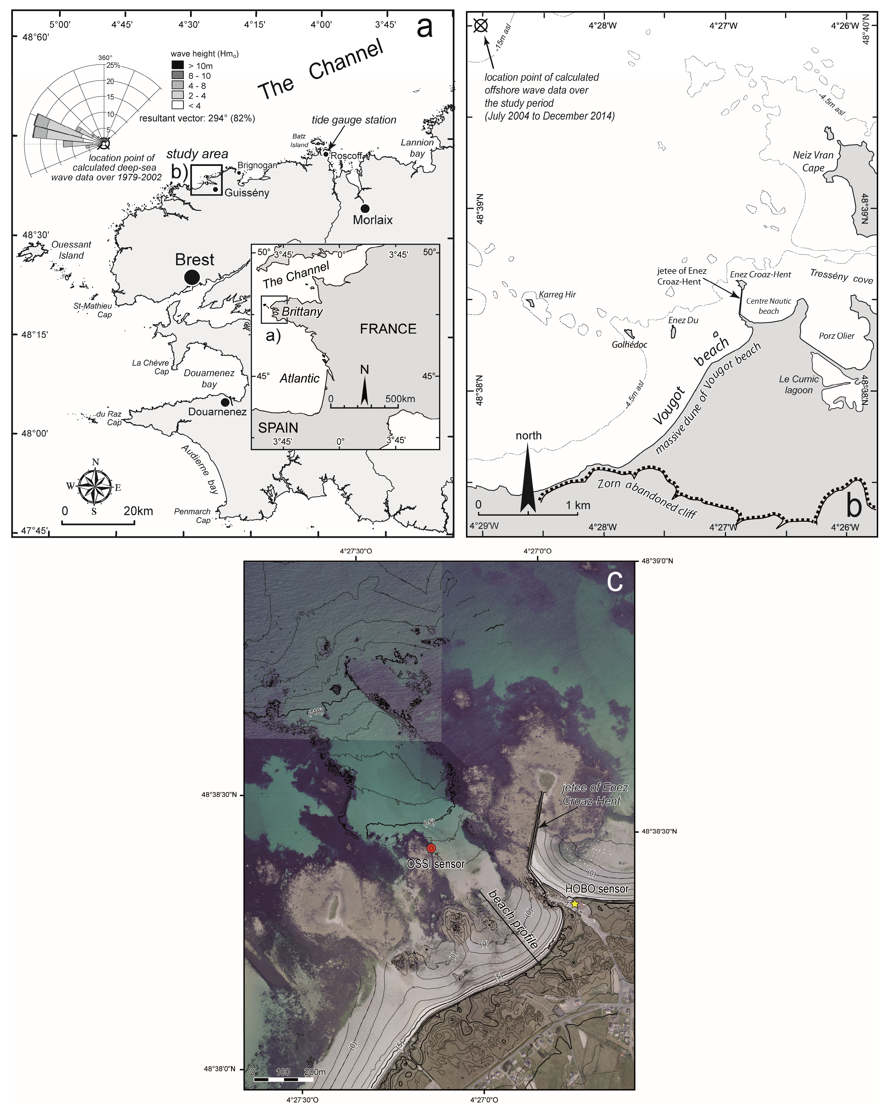
2. Geomorphological and Hydrodynamic Setting

The study area is the Vougot beach located on the North coast of Finistère in Brittany (France) (Figure 2). The general morphological setting comprises large rocky outcrops representing the submerged part of the Léon plateau. Contact between the coastal platform and the continental part of the plateau consists of a partly tectonic scarp 30 to 50 m high. In the Vougot beach area, the scarp is disconnected from the sea by the existence of a dune which was formed during the Holocene [34]. This dune, anchored on the Zorn abandoned cliff, stretches over about 2 km in a southwest to northeast direction (Figure 2b). It culminates at an altitude of 13 m (NGF) (i.e., above sea level—asl); the altimetric reference NGF refers to French datum. In our case this reference is situated 3.5 m above the lowest astronomic tide level (LAT). It represents a massive dune complex 250 to 400 m wide. Over the last decades, the dune of Vougot beach has experienced erosion. A historical shoreline change analysis based on a series of aerial photographs and field measurements from 1952 to 2014 shows that the retreat of the dune principally affected the eastern part of Vougot beach. Erosion was caused by the construction of the Enez Croas Hent jetty in 1974 (Figure 2b), which completely modified the hydrodynamics and interrupted the westward sand drift, inducing an increase in sediment loss for the Vougot beach/dune system [35]. Calculation of erosion rates over the 1978–2000 period (following the building of the jetty in 1974) showed that the maximum retreat of the dune reached −0.6 m/year; and this rate has increased from −0.6 m/year to −1.5 m/year over the last decade (from 2000 to 2009) due to the impact of a major storm on 10 March 2008 [35,36]. However, from spring 2008 to summer 2013, almost five years of dune recovery occurred. It was characterized by dune progradation reaching +12 m on the zones with the most accretion [37]. Finally, during the winter of 2013–2014, a cluster of about 12 storm events hit the coast of Brittany with an exceptional frequency [38]. Dune erosion of Vougot beach during this period (between December 2013 and March 2014) reached almost −15 m on the most retreated part. Therefore, the maximum retreat of the dune between 2008 and 2014 was about −0.7 m/year.

Figure 1. Method used by Cariolet and Suanez [33] to calculate beach slope for the runup calculation. The lower bound corresponds to the limit of the profile section where changes of elevation are the most significant. This section concerns the upper part of the profile, and it is called “active section”. This limit of 43 m has been defined by calculating the standard deviation of height changes of the beach profiles (gray lines) measured between April 2008 and November 2010 (see Table 1). The upper bound corresponds to field measurements of the swash height given by the water mark limit or wrack line deposit.

Figure 1. Method used by Cariolet and Suanez [33] to calculate beach slope for the runup calculation. The lower bound corresponds to the limit of the profile section where changes of elevation are the most significant. This section concerns the upper part of the profile, and it is called “active section”. This limit of 43 m has been defined by calculating the standard deviation of height changes of the beach profiles (gray lines) measured between April 2008 and November 2010 (see Table 1). The upper bound corresponds to field measurements of the swash height given by the water mark limit or wrack line deposit.

Figure 2. Location map. Regional setting and Roscoff tidal gauge station (a); local setting and location point where offshore wave data (H_m0 and T_m0,–1) were calculated using (WW3) modeling (b); and aerial photography of Vougot beach showing the beach/dune profile location and both wave/water level and atmospheric pressure sensors (c).

Figure 2. Location map. Regional setting and Roscoff tidal gauge station (a); local setting and location point where offshore wave data (H_m0 and T_m0,–1) were calculated using (WW3) modeling (b); and aerial photography of Vougot beach showing the beach/dune profile location and both wave/water level and atmospheric pressure sensors (c).

Offshore incident waves obtained over the period 1979–2002 show that they come mostly from the west–northwest direction (242°) (Figure 2a). The most frequent wave height (H_m0) is between 1.5 and 3 m with an average height reaching 2.2 m, and the most frequent period (T_pic) is between 9 and 11 s, with an average period of 10.6 s. The maximum wave height and period related to storm events reached respectively 14 m and 20 s. Because of a tidal range reaching about 7 m between MHWS and MLWS, the Vougot beach is characterized as a macrotidal environment. The beach profile of the section studied is characterized by different morphodynamic environments according to the composite slope and concave beach (Figure 3). The lower part of the tidal beach, between MHWN and MLWN, is mainly associated with low Iribarren parameter values of ≤0.3 and a very gentle slope, tanβ, reaching 0.034 to 0.014. These morphodynamic conditions correspond to a dissipative environment. In contrast, the upper beach, between MHWN and HAT, is characterized by intermediate conditions with Iribarren values >0.72 and beach slope tanβ reaching 0.18 between HAT level and the foot of the dune. Therefore, depending on the tide’s water level, waves break at high tide on different morphodynamic environments. Under neap tide conditions, wave-breaking processes are related to rather dissipative conditions, while under spring tides, intermediate to moderately reflective conditions (Iribarren parameters up to 1.6) prevail. This environmental context is important because the behavior of runup under dissipative conditions is different than during reflective and intermediate conditions [21,39].

Figure 3. (Red line): Mean cross-shore profile of the surveyed Vougot beach section. (Blue spot): The standard deviation of profile elevation change rates (see Figure 1). Morphodynamic conditions (dissipative to reflective conditions) have been analyzed along the concave beach profile using Iribarren value.

Figure 3. (Red line): Mean cross-shore profile of the surveyed Vougot beach section. (Blue spot): The standard deviation of profile elevation change rates (see Figure 1). Morphodynamic conditions (dissipative to reflective conditions) have been analyzed along the concave beach profile using Iribarren value.

3. Methods

3.1. Monitoring of Dune Morphological Changes

The monthly monitoring of dune morphological changes started in July 2004. It consisted of beach/dune profile measurements carried out along the cross-shore transect presented in Figure 2c, using a Trimble 5700/5800 Differential GPS. Data points described by three coordinate values (x, y, z) were collected in Real Time Kinematic (RTK) mode. Measurements were calibrated using the geodesic marker from the French datum and the geodesic network provided by the IGN located about 2 km from the study area. Several control points set up in the field were used to assess the accuracy of the survey reaching ±4–5 cm (X and Y) and ±1–2 cm (Z). These values were used to calculate the margin of error associated with the dune sediment budget.

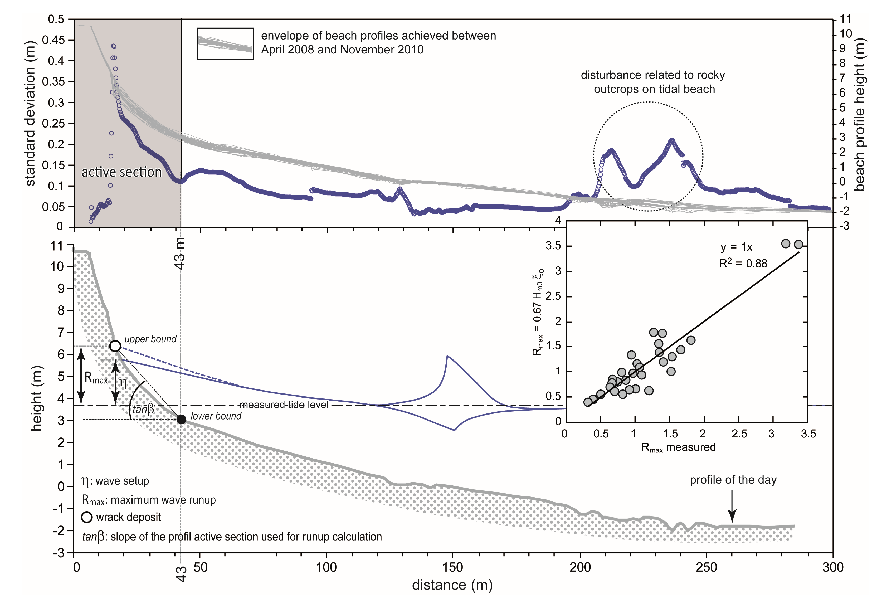
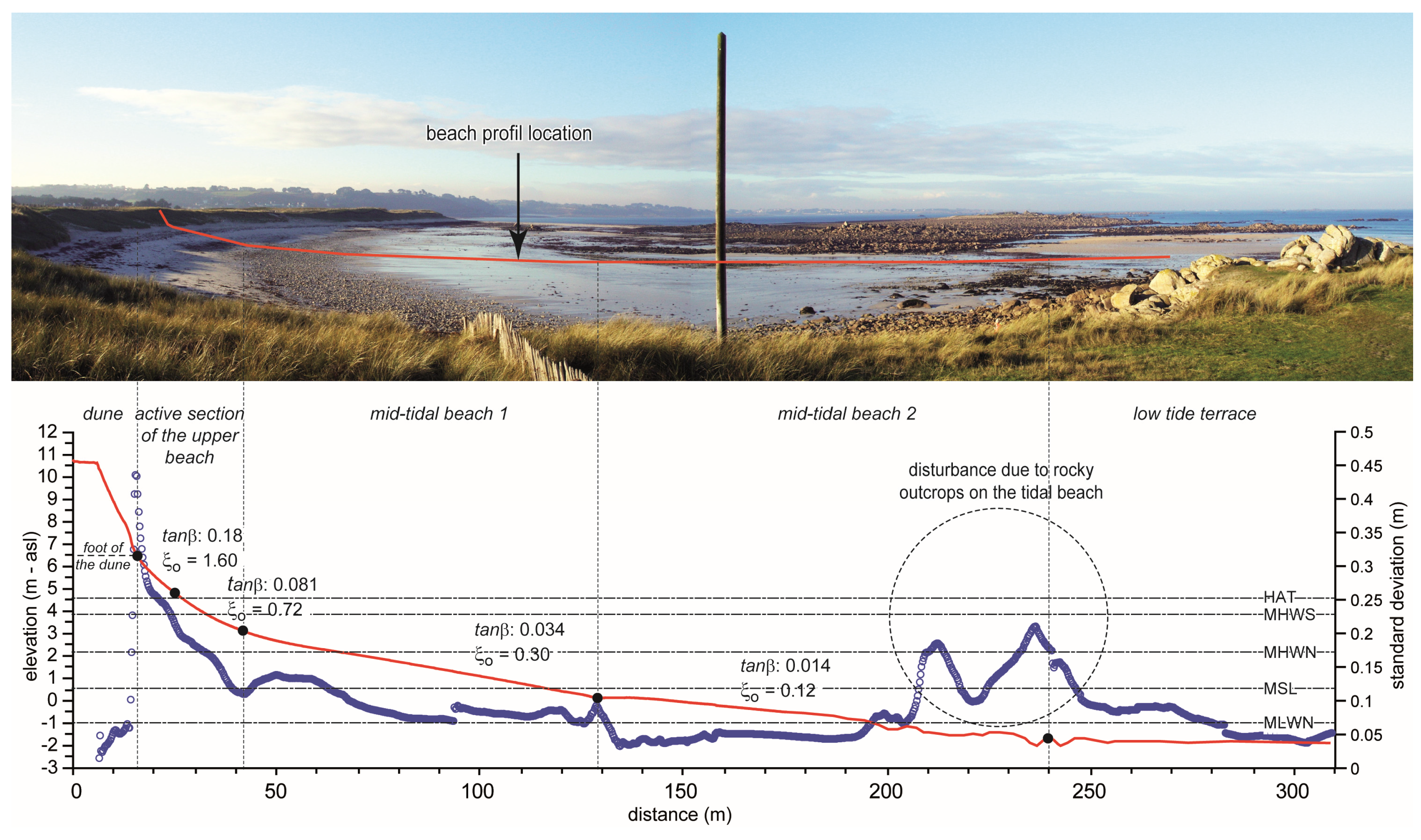
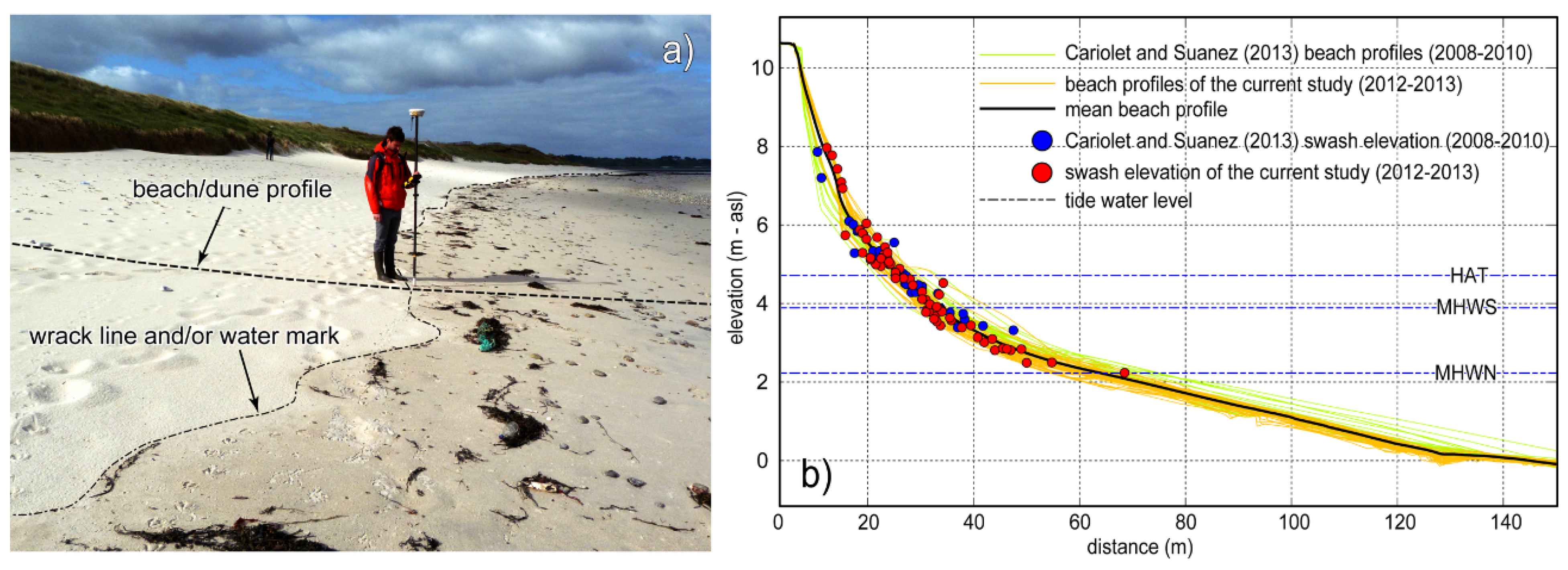
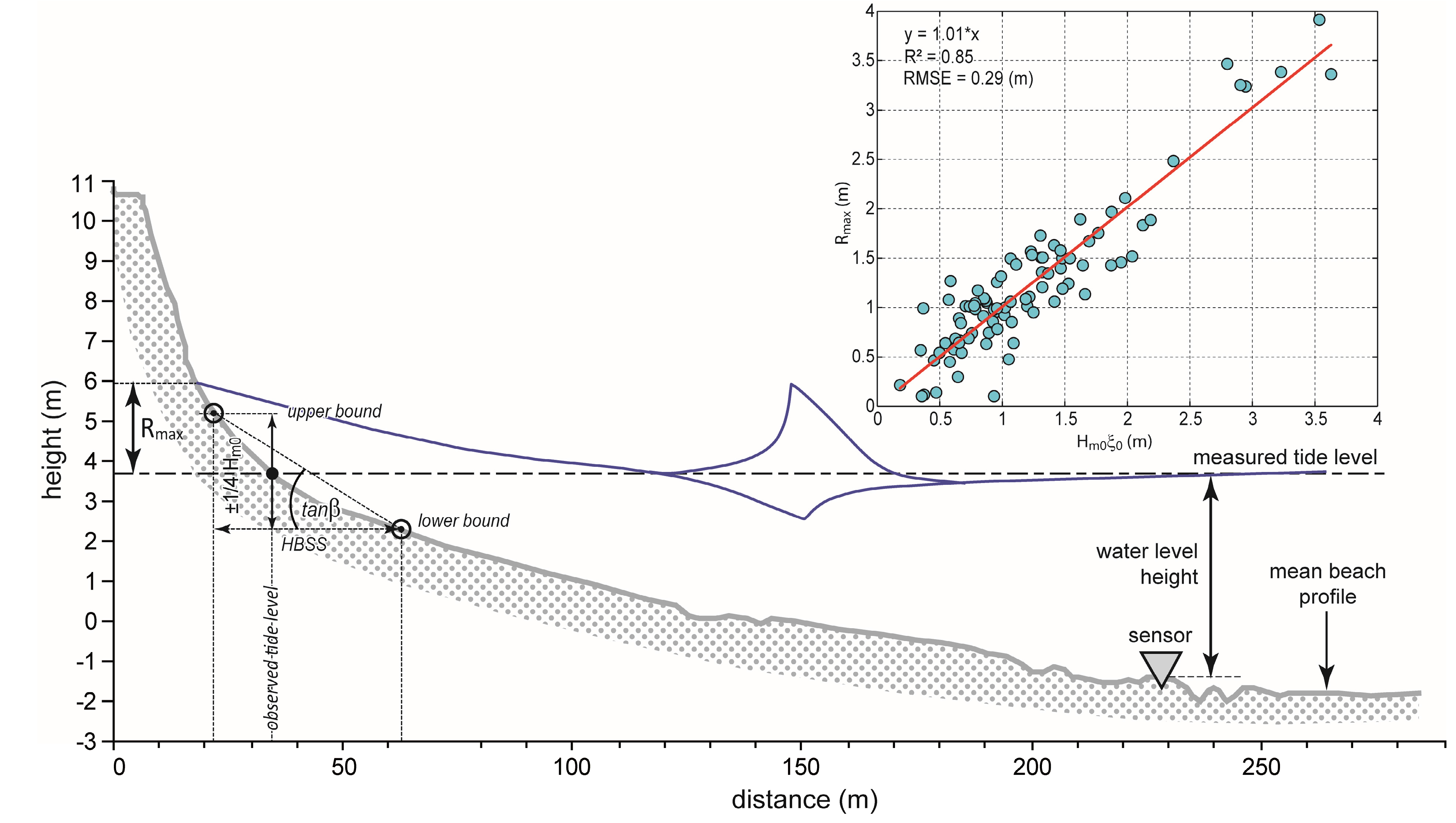
3.2. Survey of Beach Profile and Maximum Swash Elevation (Runup) R_max

Between July 2012 and June 2013, 59 measurements of beach profile and maximum swash elevation were carried out using the same method as the one followed in the previous study by Cariolet and Suanez [33]. Maximum swash elevation was determined by the wrack deposit and/or the limit of the water mark identified by a tonal change from dark wet foreshore sand to light dry sand on the upper beach (Figure 4a). We assume that this limit corresponded to the highest level reached by the runup during the previous high tide. Therefore, it corresponds to R_max (maximum runup) instead of the generally used random variable R_2% that corresponds to vertical runup distance exceeded by two percent of wave runups. In addition to the swash elevation measurement, the beach/dune profile was also measured in order to recover the morphological parameters needed to analyze runup processes. These measurements were acquired along the same transect and according to the same DGPS method as described previously. This data set was added to the 31 surveys conducted as part of the study of Cariolet and Suanez [33]. In total, a set of 90 morphological and runup measurements was used in this study (Figure 4b and Table 1).

Figure 4. The limit between dry and wet sand (water mark) at the level of high tide deposit (wrack line) shows the level reached by the swash processes (a); DGPS measurement of beach/dune profiles and the maximum runup elevation reached during the previous high tide (b).

Figure 4. The limit between dry and wet sand (water mark) at the level of high tide deposit (wrack line) shows the level reached by the swash processes (a); DGPS measurement of beach/dune profiles and the maximum runup elevation reached during the previous high tide (b).

Table 1. Overview of environmental conditions and dimensional swash parameters where H_m0 (m), T_m0,–1 (s), and L₀ (m) correspond to WW3 offshore wave, R_max (m) is runup field measurements, and HTWL (m) is high tide water level.

Date	Hm0 (m)	Tm0,–1 (s)	L0 (m)	Slope (tanβ)	ξ0	Rmax (m)	HTWL (m)
08 April 2008	0.6	8.1	101	0.118	1.502	0.95	4.36
29 August 2008	1.0	8.3	107	0.061	0.623	0.30	3.10
29 September 2008	0.8	7.5	88	0.093	1.004	0.74	3.80
12 January 2009	3.6	12.9	261	0.096	0.825	3.24	4.01
13 February 2009	1.8	11.0	188	0.107	1.111	1.46	4.14
29 April 2009	1.7	8.7	119	0.071	0.591	0.93	3.37
17 December 2009	0.8	10.0	156	0.080	1.100	0.75	3.56
22 December 2009	1.0	8.0	101	0.067	0.680	0.67	3.22
23 December 2009	1.0	7.9	98	0.056	0.559	0.64	2.97
30 December 2009	1.6	10.5	171	0.073	0.749	1.11	3.40
04 January 2010	1.6	8.3	107	0.110	0.906	1.06	4.19
07 January 2010	2.3	6.6	69	0.058	0.319	0.69	3.09
13 January 2010	2.8	11.6	210	0.054	0.462	1.36	3.03
14 January 2010	2.6	11.8	217	0.069	0.635	1.43	3.36
16 January 2010	2.3	11.9	223	0.091	0.903	1.52	3.83
21 January 2010	2.8	12.9	261	0.054	0.525	1.40	3.04
28 January 2010	2.0	7.5	88	0.049	0.324	0.89	2.86
01 February 2010	1.5	6.6	68	0.123	0.837	1.57	4.53
03 February 2010	1.8	7.6	90	0.111	0.781	1.63	4.23
05 February 2010	2.9	11.5	207	0.068	0.570	1.14	3.35
05 February 2010	4.5	13.5	285	0.049	0.393	1.75	2.95
06 February 2010	4.1	12.0	226	0.039	0.293	1.02	2.41
26 February 2010	2.1	6.0	56	0.065	0.336	1.01	3.24
28 February 2010	1.5	5.6	50	0.124	0.710	1.50	4.56
03 March 2010	1.1	5.7	50	0.127	0.846	1.26	4.62
29 March 2010	1.2	7.6	89	0.113	0.965	1.08	4.28
31 March 2010	4.5	9.2	132	0.114	0.616	3.47	4.52
10 June 2010	1.3	6.2	61	0.051	0.347	0.47	2.87
13 July 2010	1.1	8.6	116	0.097	0.991	0.64	3.89
12 October 2010	1.8	6.3	62	0.082	0.482	0.63	3.61
08 November 2010	2.6	7.3	82	0.115	0.648	1.67	4.39
05 July 2012	1.7	9.2	132	0.097	0.847	1.50	3.95
02 October 2012	2.6	10.7	180	0.086	0.712	1.97	3.73
17 October 2012	3.6	12.5	246	0.123	1.018	3.36	4.63
02 November 2012	2.8	8.9	123	0.080	0.531	1.58	3.60
06 November 2012	1.5	6.8	72	0.033	0.225	0.57	2.24
12 November 2012	1.9	9.7	146	0.078	0.686	1.73	3.52
19 November 2012	1.6	9.3	134	0.076	0.697	1.44	3.46
23 November 2012	3.3	11.5	205	0.039	0.306	1.00	2.45
26 November 2012	2.4	8.5	112	0.065	0.440	1.06	3.25
30 November 2012	1.0	9.6	144	0.077	0.903	0.10	3.49
03 December 2012	3.0	10.4	170	0.058	0.434	1.51	3.13
06 December 2012	1.7	10.0	157	0.036	0.337	1.27	2.39
11 December 2012	1.1	7.6	89	0.063	0.575	0.68	3.15
13 December 2012	0.8	10.8	183	0.107	1.584	1.21	4.13
14 December 2012	1.8	11.3	198	0.125	1.304	2.48	4.64
17 December 2012	4.8	12.2	233	0.097	0.678	3.38	4.14
07 January 2013	1.8	10.8	181	0.034	0.337	0.58	2.25
08 January 2013	1.8	10.8	184	0.038	0.384	0.55	2.50
09 January 2013	1.8	12.1	227	0.053	0.596	0.47	2.92
16 January 2013	1.1	6.7	71	0.098	0.774	1.05	3.91
23 January 2013	4.0	13.1	266	0.038	0.312	1.54	2.33
24 January 2013	2.4	10.9	187	0.041	0.362	1.07	2.63
25 January 2013	2.1	11.2	195	0.053	0.502	0.85	2.95
27 January 2013	3.1	10.1	160	0.089	0.635	2.11	3.81
28 January 2013	5.1	13.9	301	0.074	0.567	3.25	3.68
29 January 2013	5.0	14.3	318	0.089	0.708	3.91	3.98
04 February 2013	2.7	9.4	139	0.038	0.270	1.01	2.43
05 February 2013	5.7	11.9	220	0.039	0.241	1.35	2.20
06 February 2013	6.1	12.4	242	0.040	0.251	1.50	2.29
07 February 2013	3.3	9.3	136	0.040	0.259	1.09	2.53
14 February 2013	3.1	10.2	163	0.094	0.678	1.83	3.93
19 February 2013	1.8	12.5	242	0.031	0.361	0.65	1.60
21 February 2013	1.5	7.4	87	0.032	0.240	0.99	1.87
22 February 2013	1.9	8.5	112	0.034	0.266	0.54	2.30
04 March 2013	0.9	5.6	49	0.057	0.422	0.12	2.99
05 March 2013	0.5	4.8	36	0.042	0.359	0.22	2.63
10 March 2013	1.5	12.7	250	0.095	1.211	1.43	3.89
14 March 2013	1.2	5.5	48	0.104	0.656	0.98	4.04
28 March 2013	0.9	7.2	82	0.109	1.038	0.98	4.17
29 March 2013	0.9	6.8	73	0.116	1.058	0.86	4.32
08 April 2013	1.9	11.1	191	0.081	0.814	1.24	3.57
09 April 2013	2.0	8.4	111	0.099	0.734	1.19	3.98
07 May 2013	1.7	12.4	241	0.062	0.747	0.95	3.15
09 May 2013	2.4	9.0	126	0.076	0.546	1.51	3.50
23 May 2013	1.5	6.8	73	0.063	0.438	0.84	3.17
23 May 2013	2.2	6.4	65	0.072	0.396	1.09	3.40
24 May 2013	1.8	6.2	60	0.077	0.440	1.17	3.49
25 May 2013	2.1	6.3	63	0.086	0.466	1.32	3.71
27 May 2013	0.6	7.6	91	0.104	1.246	1.04	4.04
12 June 2013	1.6	8.2	106	0.060	0.499	1.02	3.10
13 June 2013	2.8	9.3	135	0.049	0.344	0.99	2.92
14 June 2013	1.4	8.6	114	0.045	0.405	1.08	2.73
18 June 2013	0.9	9.1	128	0.034	0.408	0.10	2.39
19 June 2013	1.9	7.8	94	0.035	0.249	0.14	2.36
20 June 2013	1.9	7.9	97	0.043	0.305	0.45	2.69
21 June 2013	1.6	9.4	138	0.057	0.530	0.91	3.02
23 June 2013	3.8	9.9	154	0.091	0.578	1.89	3.91
24 June 2013	2.7	8.9	124	0.089	0.605	1.89	3.79
25 June 2013	1.1	7.8	95	0.096	0.911	0.78	3.89

Table 1. Overview of environmental conditions and dimensional swash parameters where H_m0 (m), T_m0,–1 (s), and L₀ (m) correspond to WW3 offshore wave, R_max (m) is runup field measurements, and HTWL (m) is high tide water level.

Date	Hm0 (m)	Tm0,–1 (s)	L0 (m)	Slope (tanβ)	ξ0	Rmax (m)	HTWL (m)
08 April 2008	0.6	8.1	101	0.118	1.502	0.95	4.36
29 August 2008	1.0	8.3	107	0.061	0.623	0.30	3.10
29 September 2008	0.8	7.5	88	0.093	1.004	0.74	3.80
12 January 2009	3.6	12.9	261	0.096	0.825	3.24	4.01
13 February 2009	1.8	11.0	188	0.107	1.111	1.46	4.14
29 April 2009	1.7	8.7	119	0.071	0.591	0.93	3.37
17 December 2009	0.8	10.0	156	0.080	1.100	0.75	3.56
22 December 2009	1.0	8.0	101	0.067	0.680	0.67	3.22
23 December 2009	1.0	7.9	98	0.056	0.559	0.64	2.97
30 December 2009	1.6	10.5	171	0.073	0.749	1.11	3.40
04 January 2010	1.6	8.3	107	0.110	0.906	1.06	4.19
07 January 2010	2.3	6.6	69	0.058	0.319	0.69	3.09
13 January 2010	2.8	11.6	210	0.054	0.462	1.36	3.03
14 January 2010	2.6	11.8	217	0.069	0.635	1.43	3.36
16 January 2010	2.3	11.9	223	0.091	0.903	1.52	3.83
21 January 2010	2.8	12.9	261	0.054	0.525	1.40	3.04
28 January 2010	2.0	7.5	88	0.049	0.324	0.89	2.86
01 February 2010	1.5	6.6	68	0.123	0.837	1.57	4.53
03 February 2010	1.8	7.6	90	0.111	0.781	1.63	4.23
05 February 2010	2.9	11.5	207	0.068	0.570	1.14	3.35
05 February 2010	4.5	13.5	285	0.049	0.393	1.75	2.95
06 February 2010	4.1	12.0	226	0.039	0.293	1.02	2.41
26 February 2010	2.1	6.0	56	0.065	0.336	1.01	3.24
28 February 2010	1.5	5.6	50	0.124	0.710	1.50	4.56
03 March 2010	1.1	5.7	50	0.127	0.846	1.26	4.62
29 March 2010	1.2	7.6	89	0.113	0.965	1.08	4.28
31 March 2010	4.5	9.2	132	0.114	0.616	3.47	4.52
10 June 2010	1.3	6.2	61	0.051	0.347	0.47	2.87
13 July 2010	1.1	8.6	116	0.097	0.991	0.64	3.89
12 October 2010	1.8	6.3	62	0.082	0.482	0.63	3.61
08 November 2010	2.6	7.3	82	0.115	0.648	1.67	4.39
05 July 2012	1.7	9.2	132	0.097	0.847	1.50	3.95
02 October 2012	2.6	10.7	180	0.086	0.712	1.97	3.73
17 October 2012	3.6	12.5	246	0.123	1.018	3.36	4.63
02 November 2012	2.8	8.9	123	0.080	0.531	1.58	3.60
06 November 2012	1.5	6.8	72	0.033	0.225	0.57	2.24
12 November 2012	1.9	9.7	146	0.078	0.686	1.73	3.52
19 November 2012	1.6	9.3	134	0.076	0.697	1.44	3.46
23 November 2012	3.3	11.5	205	0.039	0.306	1.00	2.45
26 November 2012	2.4	8.5	112	0.065	0.440	1.06	3.25
30 November 2012	1.0	9.6	144	0.077	0.903	0.10	3.49
03 December 2012	3.0	10.4	170	0.058	0.434	1.51	3.13
06 December 2012	1.7	10.0	157	0.036	0.337	1.27	2.39
11 December 2012	1.1	7.6	89	0.063	0.575	0.68	3.15
13 December 2012	0.8	10.8	183	0.107	1.584	1.21	4.13
14 December 2012	1.8	11.3	198	0.125	1.304	2.48	4.64
17 December 2012	4.8	12.2	233	0.097	0.678	3.38	4.14
07 January 2013	1.8	10.8	181	0.034	0.337	0.58	2.25
08 January 2013	1.8	10.8	184	0.038	0.384	0.55	2.50
09 January 2013	1.8	12.1	227	0.053	0.596	0.47	2.92
16 January 2013	1.1	6.7	71	0.098	0.774	1.05	3.91
23 January 2013	4.0	13.1	266	0.038	0.312	1.54	2.33
24 January 2013	2.4	10.9	187	0.041	0.362	1.07	2.63
25 January 2013	2.1	11.2	195	0.053	0.502	0.85	2.95
27 January 2013	3.1	10.1	160	0.089	0.635	2.11	3.81
28 January 2013	5.1	13.9	301	0.074	0.567	3.25	3.68
29 January 2013	5.0	14.3	318	0.089	0.708	3.91	3.98
04 February 2013	2.7	9.4	139	0.038	0.270	1.01	2.43
05 February 2013	5.7	11.9	220	0.039	0.241	1.35	2.20
06 February 2013	6.1	12.4	242	0.040	0.251	1.50	2.29
07 February 2013	3.3	9.3	136	0.040	0.259	1.09	2.53
14 February 2013	3.1	10.2	163	0.094	0.678	1.83	3.93
19 February 2013	1.8	12.5	242	0.031	0.361	0.65	1.60
21 February 2013	1.5	7.4	87	0.032	0.240	0.99	1.87
22 February 2013	1.9	8.5	112	0.034	0.266	0.54	2.30
04 March 2013	0.9	5.6	49	0.057	0.422	0.12	2.99
05 March 2013	0.5	4.8	36	0.042	0.359	0.22	2.63
10 March 2013	1.5	12.7	250	0.095	1.211	1.43	3.89
14 March 2013	1.2	5.5	48	0.104	0.656	0.98	4.04
28 March 2013	0.9	7.2	82	0.109	1.038	0.98	4.17
29 March 2013	0.9	6.8	73	0.116	1.058	0.86	4.32
08 April 2013	1.9	11.1	191	0.081	0.814	1.24	3.57
09 April 2013	2.0	8.4	111	0.099	0.734	1.19	3.98
07 May 2013	1.7	12.4	241	0.062	0.747	0.95	3.15
09 May 2013	2.4	9.0	126	0.076	0.546	1.51	3.50
23 May 2013	1.5	6.8	73	0.063	0.438	0.84	3.17
23 May 2013	2.2	6.4	65	0.072	0.396	1.09	3.40
24 May 2013	1.8	6.2	60	0.077	0.440	1.17	3.49
25 May 2013	2.1	6.3	63	0.086	0.466	1.32	3.71
27 May 2013	0.6	7.6	91	0.104	1.246	1.04	4.04
12 June 2013	1.6	8.2	106	0.060	0.499	1.02	3.10
13 June 2013	2.8	9.3	135	0.049	0.344	0.99	2.92
14 June 2013	1.4	8.6	114	0.045	0.405	1.08	2.73
18 June 2013	0.9	9.1	128	0.034	0.408	0.10	2.39
19 June 2013	1.9	7.8	94	0.035	0.249	0.14	2.36
20 June 2013	1.9	7.9	97	0.043	0.305	0.45	2.69
21 June 2013	1.6	9.4	138	0.057	0.530	0.91	3.02
23 June 2013	3.8	9.9	154	0.091	0.578	1.89	3.91
24 June 2013	2.7	8.9	124	0.089	0.605	1.89	3.79
25 June 2013	1.1	7.8	95	0.096	0.911	0.78	3.89

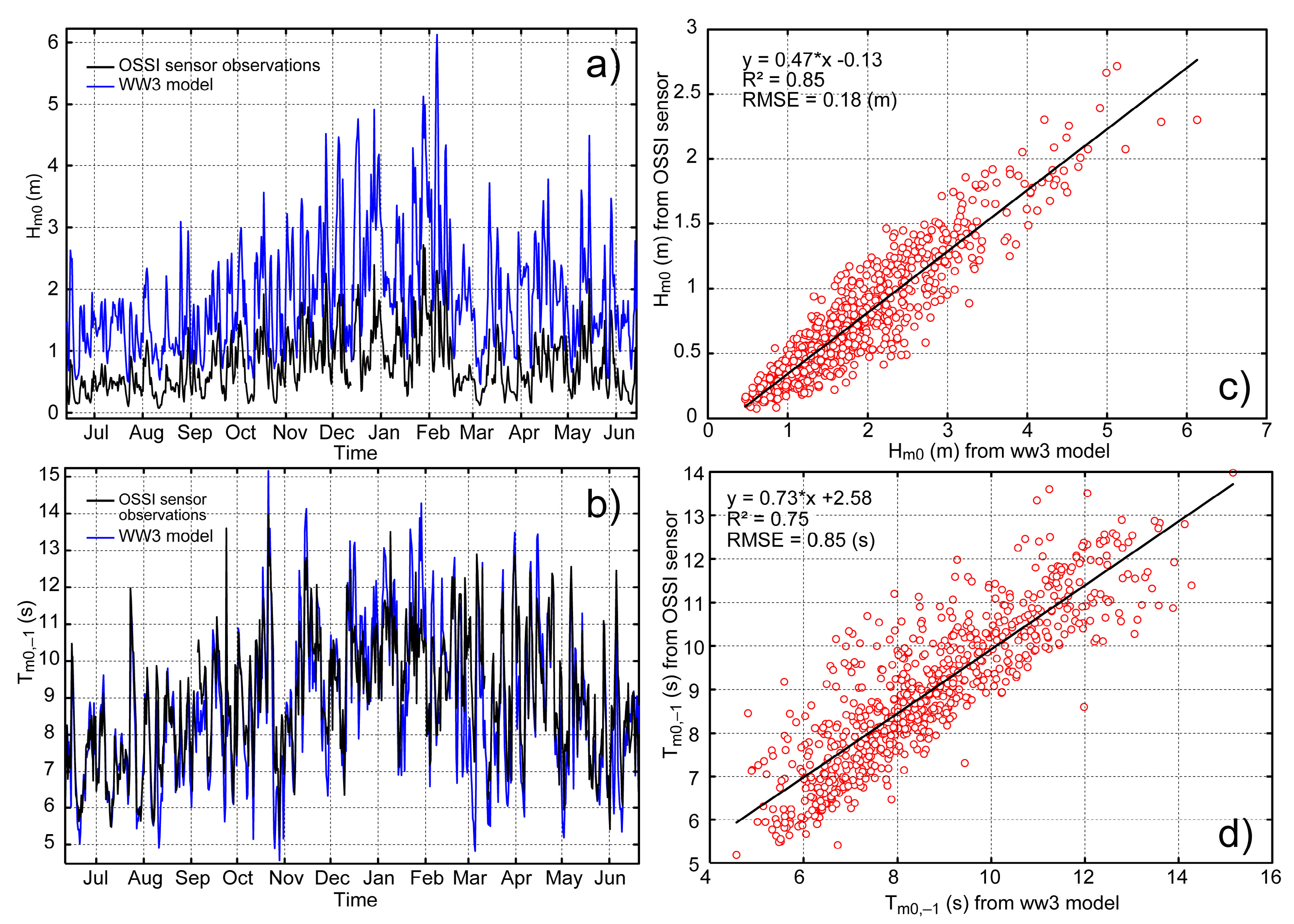
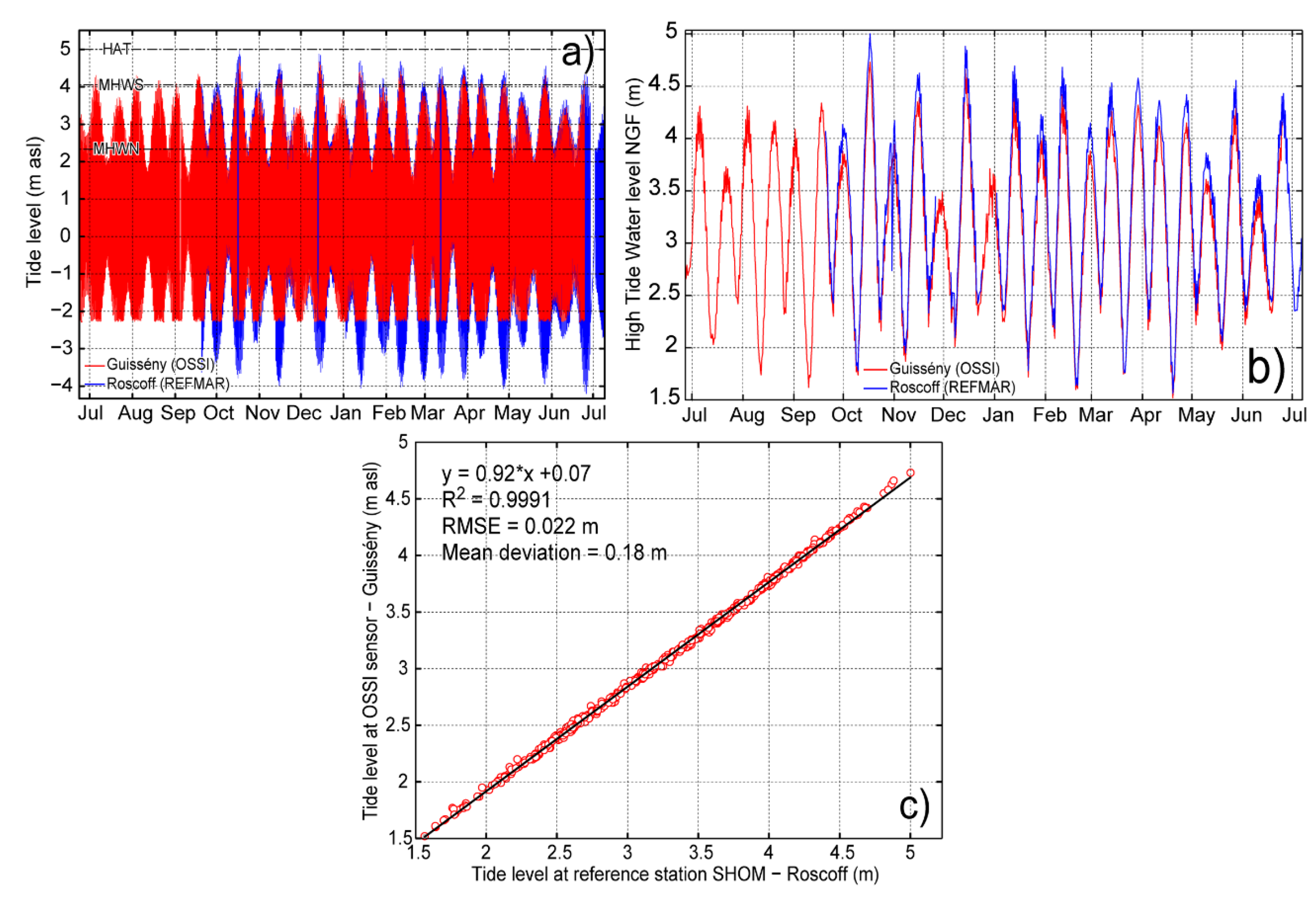
3.3. Hydrodynamic Condition Measurements

Wave analysis is based on two data sets acquired between June 2012 and June 2013. The first one corresponds to records taken on the intertidal zone using the OSSI-010-003C pressure sensor (accuracy ±1.5 cm specification) (Ocean Sensor Systems, Inc^®, Coral Springs, FL, USA), which was deployed along the morphological profile mentioned above, at −2.5 m asl which corresponds about to the low water spring tide level (Figure 2c). A recording frequency of 5 Hz was chosen to reproduce as accurately as possible the wave spectrum. The sensor was calibrated before and after each deployment by comparing the pressure measured at the low tide level (when the sensor is out of the water and thus measures atmospheric pressure) with the atmospheric pressure recorded in situ. The atmospheric pressure was measured using the HOBO U20 Water Level Logger sensor (Onset Computer Corporation^®, Bourne, MA, USA) which was positioned on the outside wall of the nautical center (Figure 2c). The second set of wave data concerns simulations acquired from the WAVEWATCH III model (WW3), which reproduced the offshore wave conditions at the calculation point 4°29′24′′ W, 48°40′12′′ N at a water depth of 18.3 m [40,41].

Wave parameters such as wave height (H_m0) and period (T_m0,–1) were extracted from both data sets for the time periods corresponding to the high tide level (Figure 5). Results showed that the monitoring period was marked by a high variability of hydrodynamic conditions. Between the end of November 2012 and mid-February 2013, ten episodes marked by high offshore waves (>4 m) were recorded, including the storm of 6 February, which was characterized by significant heights of >6 m. One can also note the two episodes of 14 May and 23 June, where the swells were often above 4 m. A validation of the offshore wave data set obtained using WW3 modeling was achieved by comparing these data to those measured in the tidal zone by a wave gauge sensor. The correlation shows a good relationship between both sets of data, especially for the wave height, with, however, less correlation regarding the periods (Figure 5).

Analysis of the tides is also based on records taken in the tidal zone using gauge sensor OSSI-010-003C (Figure 2c). The observed water level was computed taking into account atmospheric pressure measured by the HOBO U20 Water Level Logger sensor (Onset Computer Corporation^®, Bourne, MA, USA) set up on the study site (Figure 2c). It was then possible to calculate the pressure exerted by the water column and thus to calculate the height of the latter with the following expression:

H _{(water level)} = (P_sensor − P_atmosphere)/ρ.g

(7)

where H is the height of the water column (in m), P_sensor is the pressure measured by the sensor (in Pa), P_atmosphere is the atmospheric pressure (in Pa), ρ is the density of water (=1025 kg/m³), and g is the acceleration of gravity (=9.81 m/s²).

Water levels were smoothed to a moving average of 10 min to filter out deformations of the water surface related to wave action, and water levels corresponding to both daily high tides were extracted. A similar calculation was done using data recorded at a permanent tide gauge station near Roscoff located at about 30 km east of the study site (Figure 2). Both the time series from Guissény and Roscoff were used to estimate the differences in high tide water level between the two sites (Figure 6). As Figure 6b shows, more than 500 high tide level records were used for the statistical analysis, showing a very good correlation between both the Roscoff and Guissény sites. The mean deviation is 18 cm, with variations between 25 cm for spring tides and 5 cm for neap tides (Figure 6c).

Figure 5. Offshore (WW3) and shallow (OSSI) wave heights (a) and periods (b) obtained between July 2012 and June 2013. Correlations between offshore and shallow wave heights (c) and periods (d).

Figure 5. Offshore (WW3) and shallow (OSSI) wave heights (a) and periods (b) obtained between July 2012 and June 2013. Correlations between offshore and shallow wave heights (c) and periods (d).

Figure 6. Comparison between tide level (a) and daily high tide water levels (b) recorded at Vougot beach, using the OSSI-010-003C sensor, and at the permanent Roscoff tide gauge station. (c) Correlation between high tide water levels recorded at Vougot beach and at the permanent Roscoff tide gauge station.

Figure 6. Comparison between tide level (a) and daily high tide water levels (b) recorded at Vougot beach, using the OSSI-010-003C sensor, and at the permanent Roscoff tide gauge station. (c) Correlation between high tide water levels recorded at Vougot beach and at the permanent Roscoff tide gauge station.

Observed tide levels show that during the survey period some episodes characterized by high spring tide levels, with a tide coefficient close to 100 or higher, occurred (Table 2). When these events were combined with a storm, the measurement of runup elevation was considerably higher because of the storm surge effect. This is mainly the case for the following seven episodes: 17 October and 17 December of 2012, 29 January, 11 February, 11 March, 28 May, and 23 June of 2013.

Table 2. Inventory of high spring tide events characterized by a tide coefficient ≥100. In France, the magnitude of the tide from its average value is indicated by a coefficient expressed in hundredths, which lies between 20 and 120. A coefficient of 100 is associated with a maximum astronomical tidal range in Brest, calculated by the Service Hydrographique et Océanographique de la Marine (SHOM). It is defined as follows: C = (H − N_o)/U, where, H: high tide water level, N_o: mean water level at Brest: 4.13 m, U: height unit specific to the locality at Brest: 3.05 m. Tidal coefficients higher than 70 correspond to spring tides, below 70 they correspond to neap tides. A tidal coefficient of 95 corresponds to mean spring tide level, 45 corresponds to mean neap tide level.

Date and High Tide Time	Tide Coefficient	Predicted Tide Level (m)	Observed Tide Level (m)	Surge (m)
17/09/2012—(17:25)	104	4.3	4.34	0.04
18/09/2012—(18:15)	106	4.29	4.27	−0.02
19/09/2012—(06:20)	103	4.13	4.07	−0.06
16/10/2012—(10:30)	107	4.27
17/10/2012—(05:20)	109	4.36	4.73	0.37
18/10/2012—(06:05)	105	4.29	4.55	0.26
14/11/2012—(04:15)	104	4.26	4.22	−0.04
15/11/2012—(05:00)	107	4.40	4.35	−0.05
16/11/2012—(05:55)	104	4.36	4.39	0.03
14/12/2012—(04:50)	104	4.32	4.66	0.34
15/12/2012—(05:40)	104	4.38	4.58	0.20
12/01/2013—(04:30)	102	4.23	4.38	0.15
13/01/2013—(05:20)	106	4.39	4.42	0.03
14/01/2013—(06:11)	104	4.37	4.31	−0.04
11/02/2013—(05:11)	106	4.33	4.42	0.09
12/02/2013—05:52)	106	4.35	4.32	−0.03
12/03/2013—(04:50)	102	4.14
13/03/2013—(05:27)	103	4.16	4.26	0.1
28/03/2013—(17:20)	103	4.06	4.22	0.16
29/03/2013—(05:40)	105	4.16	4.32	0.16
26/04/2013—(16:55)	103	4.12	4.05	−0.07
27/04/2013—(17:35)	106	4.18	4.15	−0.03
26/05/2013—(17:20)	104	4.2	4.22	0.02
27/05/2013—(18:15)	104	4.16	4.31	0.15
24/06/2013—(17:15)	102	4.22	4.16	−0.06
25/06/2013—(18:00)	105	4.27
26/06/2013—(18:49)	103	4.15

Table 2. Inventory of high spring tide events characterized by a tide coefficient ≥100. In France, the magnitude of the tide from its average value is indicated by a coefficient expressed in hundredths, which lies between 20 and 120. A coefficient of 100 is associated with a maximum astronomical tidal range in Brest, calculated by the Service Hydrographique et Océanographique de la Marine (SHOM). It is defined as follows: C = (H − N_o)/U, where, H: high tide water level, N_o: mean water level at Brest: 4.13 m, U: height unit specific to the locality at Brest: 3.05 m. Tidal coefficients higher than 70 correspond to spring tides, below 70 they correspond to neap tides. A tidal coefficient of 95 corresponds to mean spring tide level, 45 corresponds to mean neap tide level.

Date and High Tide Time	Tide Coefficient	Predicted Tide Level (m)	Observed Tide Level (m)	Surge (m)
17/09/2012—(17:25)	104	4.3	4.34	0.04
18/09/2012—(18:15)	106	4.29	4.27	−0.02
19/09/2012—(06:20)	103	4.13	4.07	−0.06
16/10/2012—(10:30)	107	4.27
17/10/2012—(05:20)	109	4.36	4.73	0.37
18/10/2012—(06:05)	105	4.29	4.55	0.26
14/11/2012—(04:15)	104	4.26	4.22	−0.04
15/11/2012—(05:00)	107	4.40	4.35	−0.05
16/11/2012—(05:55)	104	4.36	4.39	0.03
14/12/2012—(04:50)	104	4.32	4.66	0.34
15/12/2012—(05:40)	104	4.38	4.58	0.20
12/01/2013—(04:30)	102	4.23	4.38	0.15
13/01/2013—(05:20)	106	4.39	4.42	0.03
14/01/2013—(06:11)	104	4.37	4.31	−0.04
11/02/2013—(05:11)	106	4.33	4.42	0.09
12/02/2013—05:52)	106	4.35	4.32	−0.03
12/03/2013—(04:50)	102	4.14
13/03/2013—(05:27)	103	4.16	4.26	0.1
28/03/2013—(17:20)	103	4.06	4.22	0.16
29/03/2013—(05:40)	105	4.16	4.32	0.16
26/04/2013—(16:55)	103	4.12	4.05	−0.07
27/04/2013—(17:35)	106	4.18	4.15	−0.03
26/05/2013—(17:20)	104	4.2	4.22	0.02
27/05/2013—(18:15)	104	4.16	4.31	0.15
24/06/2013—(17:15)	102	4.22	4.16	−0.06
25/06/2013—(18:00)	105	4.27
26/06/2013—(18:49)	103	4.15

4. Results

4.1. Calibration of Battjes (1971) Runup Formula

Fit analysis between observed runup values and morphodynamic variables was achieved following the same methodological approach as the one used by Cariolet and Suanez [33]. Morphodynamic parameters such as H_m0ξ₀ have been used to characterize runup processes in as far as it was demonstrated that these variables were best correlated with runup when using the slope of the active section. A new correlation between observed runup and H_m0ξ₀ was calculated including the data set used by Cariolet and Suanez [33] (Figure 7). The relation can be expressed as:

R_max = 0.68H_m0ξ₀

(8)

It gives the same result as the previous Cariolet and Suanez [33] study with a constant equal to 0.68 (95% confidence intervals [0.65; 0.71]).

Figure 7. Correlation between observed runup (R_max) and H_m0ξ₀. Equation R_max = 0.68H_m0ξ₀ is obtained; it was R_max = 0.67H_m0ξ₀ from Cariolet and Suanez [33] previous study.

Figure 7. Correlation between observed runup (R_max) and H_m0ξ₀. Equation R_max = 0.68H_m0ξ₀ is obtained; it was R_max = 0.67H_m0ξ₀ from Cariolet and Suanez [33] previous study.

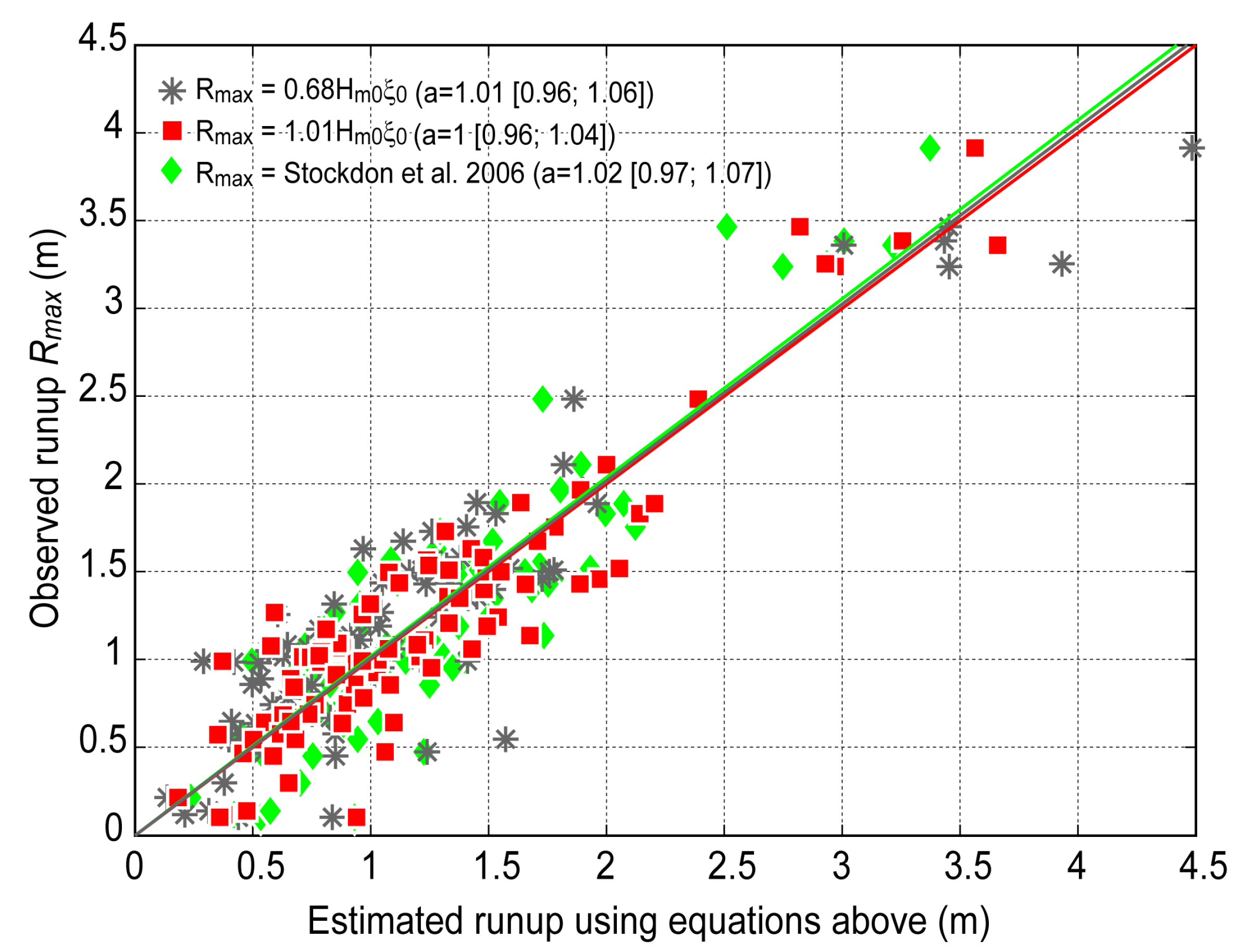
4.2. Elaboration of a General Empirical Equation

This part of the work focused on the parameterization of a general empirical equation that is no longer dependent on morphodynamic parameters obtained from high-frequency field measurements such as (i) the daily beach profile and (ii) the position of swash elevation along this profile. The approach is therefore to quantify the runup using hydrodynamic parameters such as offshore wave and water level, which are continuously recorded by wave and tide gauge stations. Morphological parameters such as the beach slope, tanβ, are meanwhile deduced from the mean beach profile assuming that the measurement of a daily beach profile is no longer taken, as we said earlier. However, the mean beach profile must be calculated from a series of measurements already available. In this case, the mean beach profile was calculated using all profile measurements recorded between June 2012 and June 2013.

Considering the previous method exposed in Section 4.1, the main problem encountered when predicting wave runup on a beach with composite-slopes (or concave shape) is how to define the upper and lower bounds of the beach profile section for which the slope is calculated when they are no longer measured on the field. Following the approach of [21,42], the slope has been calculated using the observed high tide water level (HTWL) and a fraction of the offshore wave height (H_m0) from which the horizontal beach slope section (HBSS) was defined (Figure 8). Different correlation tests have shown that 1/4H_m0 gives the best result in this case. Therefore, the upper and lower bounds of the beach slope profile width is calculated as follows

Bound_{up and low} = HTWL ± 1/4H_m0

(9)

Swash runup is in this case best parameterized with a best-fit R² (0.85) and RMSE (0.29 m). The coefficient of the regression line is 1.01 with 95% confidence intervals [0.97; 1.05]. In this case, the relationship can be expressed as (Figure 8).

R_max = 1.01H_m0ξ₀

(10)

Figure 8. Method used to calculate beach slope for the runup calculation. It is based on measured tide level from which the beach section is defined. In contrast to the previous method, note that this approach is using the mean beach profile instead of daily beach profile.

Figure 8. Method used to calculate beach slope for the runup calculation. It is based on measured tide level from which the beach section is defined. In contrast to the previous method, note that this approach is using the mean beach profile instead of daily beach profile.

The use of wave height for the calculation of HBSS gives a physical meaningful approach that is applicable from low wave energy conditions to storm wave events. The width of this beach section ranges from 3 m (H_m0 = 0.6 m and HTWL = 4.4 m asl) to 80 m (H_m0 = 6.1 m and HTWL = 2.3 m asl), with an average value of 17 m and standard deviation of 14 m (the mean of H_m0 for the dataset is 2.2 m, with standard deviation 1.2 m), depending on the position of the HTWL on the beach profile. Figure 9 shows an overview of the measured runup (R_max) dependencies of estimated runup using both Equations (8) and (10), and Equations (4)–(6) of Stockdon et al. [21]. According to the 95% confidence intervals (see Figure 9), the three correlations show that the three equations give very similar results. Nevertheless, Equation (10) best fits the observed runup.

Figure 9. Overview of the measured runup (R_max) dependencies of CH_m0ξ₀ for both Equations (8) and (10), and Equations (4)–(6) of Stockdon et al. [21].

Figure 9. Overview of the measured runup (R_max) dependencies of CH_m0ξ₀ for both Equations (8) and (10), and Equations (4)–(6) of Stockdon et al. [21].

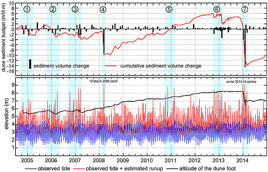
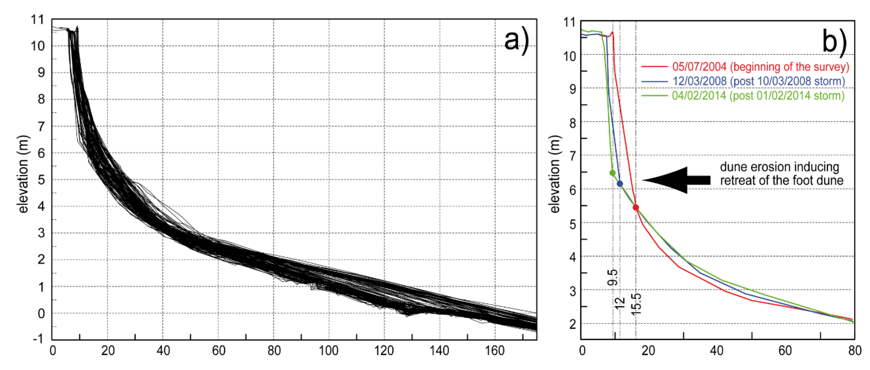
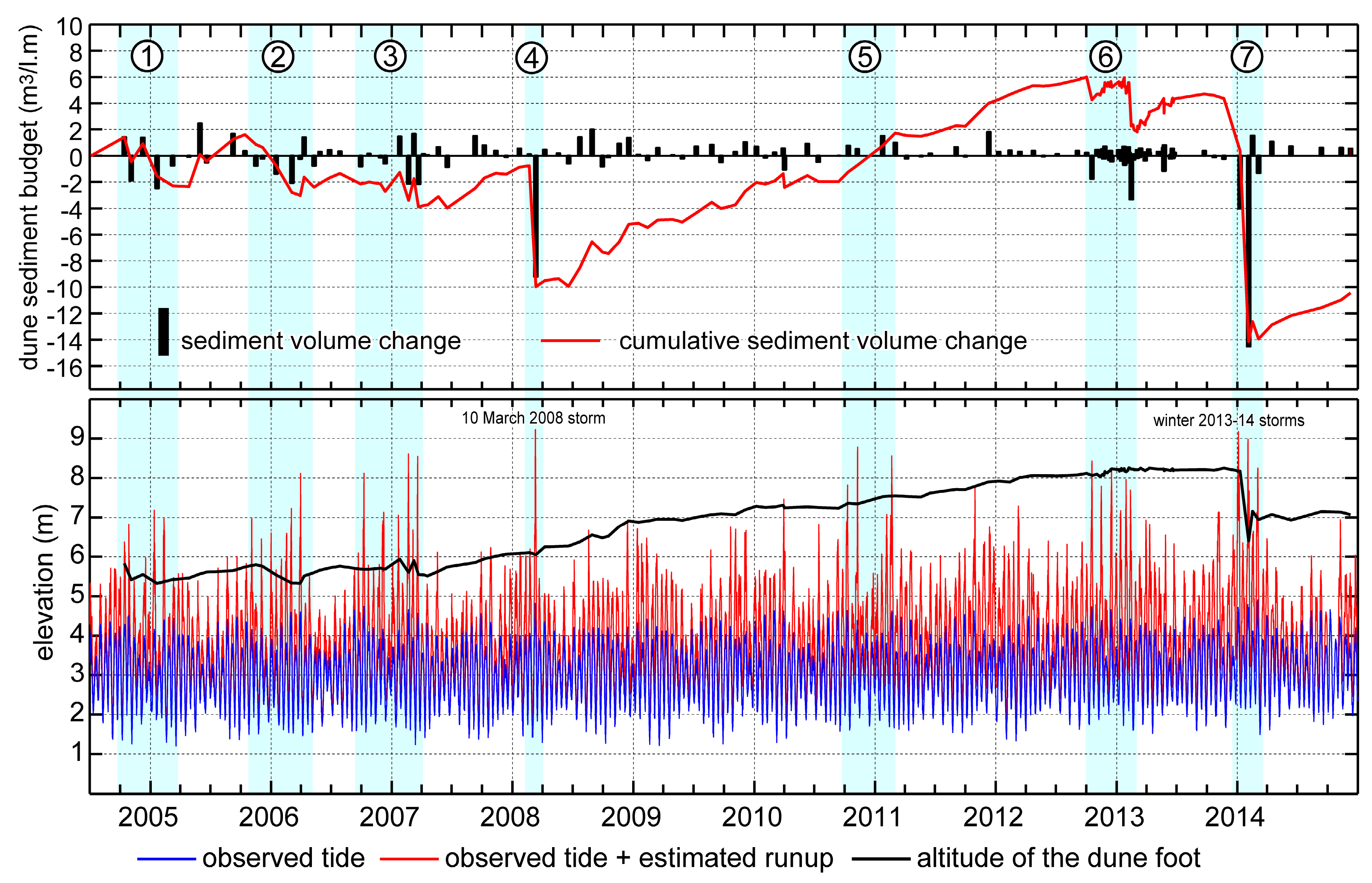
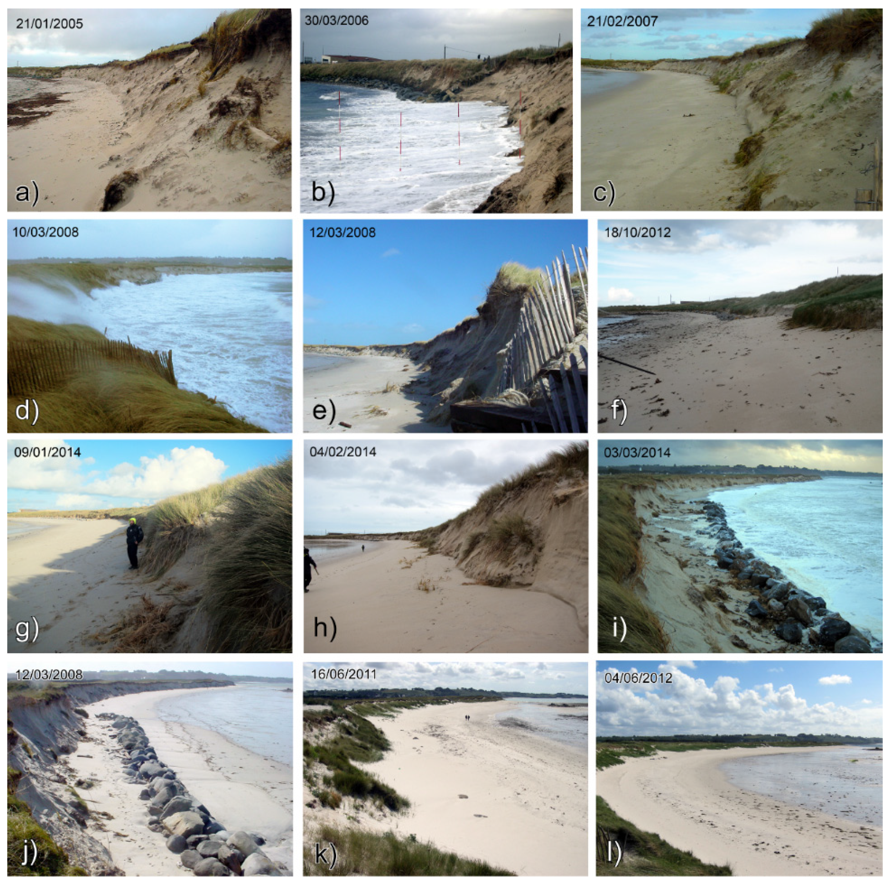
4.3. Long-Term Dune Changes Related to Storm Event Erosion and Recover

This part of the study focused on the relationship between the evolution of the dune sediment budget (in terms of accretion and erosion) and extreme water levels since July 2004. Following the “Property Erosion Model” method proposed by Ruggiero et al. [19] and/or the storm-impact scaling model proposed by Sallenger [18], the aim was to assess the sensitivity of the dune to extreme water levels by considering that erosion is experienced when the dune foot elevation is below extreme water level. Therefore, morphodynamic analysis was performed to identify the erosion stages related to extreme events, combining storm surge and high spring tide level, and on the other hand, the recover periods associated to calm wave conditions and/or low neap tide level.

Figure 10. Envelop of beach/dune profiles measured from July 2004 to December 2014 (a); The front of the dune retreated during the two main storm events, which took place during the past 10 years (i.e., 10 March 2008 and 1 February 2014) inducing landward displacement of the foot of the dune (b).

Figure 10. Envelop of beach/dune profiles measured from July 2004 to December 2014 (a); The front of the dune retreated during the two main storm events, which took place during the past 10 years (i.e., 10 March 2008 and 1 February 2014) inducing landward displacement of the foot of the dune (b).

Extreme water level was estimated for each daily high tide level by summing the swash runup elevation calculated from the Equation (10), and the measured tide level at Roscoff calibrated to the Vougot beach site. The altitude of the foot of the dune was obtained from monthly beach/dune profile measurements. However, the great morphological changes of the upper beach/dune section over the last ten years made it very difficult to identify this morphological proxy (Figure 10a). When we analyze in more detail the data set, three main phases related to strong dune erosion were identified. These three erosion phases have induced a landward displacement of the foot of the dune. As shown in Figure 10b, the foot of the dune was situated at 15.5 m from the head profile mark at the beginning of the survey. It retreated over more than 3 m during the big storm of 10 March 2008 [36,37], and retreated again over 3 m during the storm of 1 February 2014 [38]. These three reference distances (15.5 m, 12 m, and 9.5 m) were used for the calculation of the dune foot height.

Figure 11. Evolution of the dune sedimentary budget related to extreme water levels over the period from July 2004 to December 2014.

Figure 11. Evolution of the dune sedimentary budget related to extreme water levels over the period from July 2004 to December 2014.

The results show a good relationship between the negative sediment budget of the dune and phases during which extreme water levels exceed the height of the foot of the dune. On the contrary, when extreme water levels are below the height of the foot of the dune, the sediment budget increases (Figure 11). Seven phases of high extreme water levels are identified: from 28 October 2004 to 12 February 2005 (maximum water level: 7.19 m 12 January 2005), from 03 November 2005 to 31 March 2006 (maximum water level: 8.12 m 31 March 2006), from 08 October 2006 to 20 March 2007 (maximum water level: 8.61 m 20 February 2007), the 10 March 2008 storm event (9.23 m), from 09 October 2010 to 20 February 2011 (maximum water level: 8.79 m 09 November 2010), from 17 October 2012 to 11 February 2013 (maximum water level: 8.43 m 17 October 2012), and from 01 January 2014 to 03 March 2014 (maximum water level: 9.18 m 04 January 2014) (Figure 11). For six of them, extreme water levels are well-related to an erosion phase of the dune, with the exception of the period from 09 October 2010 to 20 February 2011 (Figure 12a–i). During this last period, three episodes characterized by extreme water levels higher than the foot of the dune were recorded without erosion of the dune (09 October 2010: 7.83 m; 09 November 2010: 8.79 m; 20 February 2011: 8.56 m). However, we notice that these three extreme events have occurred during a long phase of dune recovery, which started in spring 2008 (post-storm of 10 March 2008) and ended during the autumn of 2012 (Figure 12—From (j) to (l)). During these four years, the sediment budget of the dune increased considerably, inducing an elevation of the foot of the dune up to 2 m. Therefore, extreme water levels never hit the foot of the dune during this entire period except during the short stage mentioned above. The two major dune erosion stages which were recorded are related to the big storm event of 10 March 2008 [36,37], and to a cluster of storms occurring during the winter of 2013–2014 [38].

Figure 12. Photos illustrating dune erosion which occurred during the high extreme water levels phases inventoried in Figure 11: (a) post-12 January 2005 extreme water level; (b) a day before 31 March 2006 extreme water level; (c) post-20 February 2007 extreme water level; (d) 10 March 2008 storm event; (e) post-10 March 2008 storm event; (f) post-17 October 2012 extreme water level; (g) post-04 January 2014 extreme water level; (h) post-02 February 2014 extreme water level; and (i) 03 March 2014 storm event. Photos illustrating the dune recover phase post-storm of 10 March 2008 to September 2012 (j–l).

Figure 12. Photos illustrating dune erosion which occurred during the high extreme water levels phases inventoried in Figure 11: (a) post-12 January 2005 extreme water level; (b) a day before 31 March 2006 extreme water level; (c) post-20 February 2007 extreme water level; (d) 10 March 2008 storm event; (e) post-10 March 2008 storm event; (f) post-17 October 2012 extreme water level; (g) post-04 January 2014 extreme water level; (h) post-02 February 2014 extreme water level; and (i) 03 March 2014 storm event. Photos illustrating the dune recover phase post-storm of 10 March 2008 to September 2012 (j–l).

5. Discussion

Following the previous study [33], this experiment has more deeply examined new parameterization of the runup formula [1] for predicting total swash elevation in the extreme water level calculation. The focus was put on parameters that provide a first-order description of the beach morphodynamic environment, such as deep wave height (H_o), period (T), and beach steepness tanβ, which are expressed in terms of the non-dimensional surf parameter (Iribarren number ξ₀) [27]. Thus, measurements of local wave height have confirmed the validity of the use of the deep-water wave height (H_o at 18 m water depth) obtained by modeling. Similarly, in-situ measurements of water levels have improved the estimation of extreme water levels at the coast and determined the tidal range of the tide gauge shifts between Roscoff tide gauge station and the site of Guissény. The mean deviation is 18 cm, with variations between 25 cm for spring tides and 5 cm for neap tides. It is close to the 13 cm mean deviation calculated in the previous study that was based on a shorter data set and a less accurate method [33]. Concerning the beach steepness, the new set of data used in this study has confirmed the complexity of defining the best beach slope for use in the runup formula when the beach exhibits composite-slope and/or a concave profile. As demonstrated by Cariolet and Suanez [33], the slope of the active section of the upper beach gives a good fit in comparison to the field measurement (R²: 81%; RMSE of 33 cm). Nevertheless, a best-fit was obtained when beach slope was calculated using observed water level (R²: 85%; RMSE of 29 cm). This approach, based on sea level changes due to tides and/or storm surges, allows for better consideration of beach slope variations in the context of a concave beach profile. As already indicated by Mayer and Kriebel [43] the use of fixed bounds (upper or lower bounds) or an averaged planar slope for the calculation of beach steepness is therefore inappropriate when beaches exhibit complex morphology with a composite-slope, especially in a macrotidal environmental context. If we take into consideration the steep slope face of the upper concave beach (0.08 > tanβ > 1.8), this experiment also confirms the findings of Nielsen and Hanslow [32], attesting that the best-fit distribution is proportional to the surf similarity parameter (ξ_o) on intermediate to reflective beaches in agreement with Hunt’s formula for runup of regular waves on steep slopes. However, statistical tests have indicated that the reflective-specific Equation (5) of Stockdon et al. [21] was also best fitted to runup field measurements (R_max), and therefore both Equations (8) and (10).

Long-term erosion of the dune related to extreme water levels shows different pluri-decadal phases. From 2004 to 2006, the dune sediment budget indicated normal functioning characterized by erosion and high water levels during winter and accretion associated to low water levels during summer. However, dune sediment budget slightly decreased during these two first years. From the winter of 2006–2007 to the storm of 10 March 2008, the dune experienced a phase of significant sediment budget decrease related to several high extreme water level events. As mentioned earlier, this stage was followed by a long phase of dune recovery that ended during the winter of 2012–2013. The increase of the dune sediment budget was explained by supply from post-storm sediment transport between the upper intertidal beach and the lower intertidal beach—The nearshore to shoreface zone [37]. This sand supply took place during low extreme water levels associated with cold winters. The last phase was again characterized by a significant loss of dune sediment budget due to the erosion effects of the stormy winters of 2012–2013 and 2013–2014.

The inter-annual variability in dune erosion and accretion may be related to the winter North Atlantic Oscillation (NAO) index. Figure 13 presents NAO index fluctuation for the whole survey period (2004–2014). It shows three different phases that could be related to dune morphological changes. From 2000 to 2008, a positive index (denoted NAO+) is observed (Figure 13). Generally, this is associated to strong southwesterly winds that bring warm air deep into Europe. This results in mild and wet winters characterized by active storms that hit Western Europe at the latitude of England and Brittany. The winter of 1989–1990 is a good example of this weather pattern [44,45], as well as the winter of 2013–2014, during which a cluster of a dozen storms hit the Brittany coast [38,46]. In contrast, the second phase, from 2008 to 2012, is characterized by a negative index (NAO−). In this context, western European areas suffer cold dry winters and storm tracks are shifted towards the south of Europe (North Spain and Mediterranean areas). These meteorological conditions are favorable for the regeneration of dune systems because the dry weather is generally associated with effective aeolian transit to the dune. At the same time, the absence of major winter storms plays an important role in the low erosion of the dunes during these periods. The third and last phase that began in the winter of 2012–2013 is characterized by a positive NAO index. It accompanied warm and stormy winters, especially the winter of 2013–2014 [38,46]. Between December 2013 and March 2014, a cluster of about 12 storm events hit the coast of Brittany with an exceptional frequency. It was in February that these storm events were the most frequent and particularly virulent. The significant wave heights measured off Finistère reached, respectively, 12.3 and 12.4 m during the Petra and Ulla storms on 5 and 14 February. However, analysis of hydrodynamic conditions showed that only three episodes promoted extreme morphogenetic conditions because they were combined with high spring tide level. The first one occurred from 1–4 January, it was followed by events during 1–3 February, and 2 and 3 March. As indicated on Figure 12, these three events generated high extreme water levels and strong dune erosion. The maximum retreat of the front of the dune during this period reached more than −16 m [38].

Figure 13. North Atlantic Oscillation Index (NAO) from 1950 to 2015 [47].

Figure 13. North Atlantic Oscillation Index (NAO) from 1950 to 2015 [47].

Consistent with this assumption, many studies have suggested that the North Atlantic Oscillation (NAO) may control the occurrence of storm events in the Atlantic, and thus potentially influence coastal morphological changes. The role of the NAO in coastal morphological dynamics has been suggested by Masselink et al. [48] to explain medium-term outer sand bar dynamics in the southwest of England (Perranporth). It was also suggested by Thomas et al., after analyzing beach rotation at South Sands Tenby in West Wales [49,50] and O’Connor et al. [51] concerning long-term shoreline and ebb channel evolution in northwest Ireland. The same conclusion was put forward by Vespremeanu-Stroe et al. [52] who showed that shoreline changes at decadal time scales were also driven by the NAO which controls the storminess on the Danube delta coast. Nevertheless, analysis of long-term dune morphological changes on the Sefton coast (west England) indicated only a modest relationship between dune erosion/accretion rates and the North Atlantic Oscillation index [20]. The authors suggested that these dune erosion/accretion phases are also related to the long-term beach sediment budget that governs essential changes in the morphology of the nearshore and offshore zones. Similarly, Montreuil and Bullard indicated that the winter North Atlantic Oscillation phase was not a good indicator of storminess on the east coast of England but may be a useful proxy for quiescence [53]. For this specific coastal area, the authors found the Jenkinson daily weather type classification to be a better proxy for the occurrence of strong onshore storm winds.

6. Conclusions

The runup process is still relatively too complex to parameterize in a macrotidal environment where beach profiles exhibit a composite-slope. This morphology is quite often found in North Brittany along the Channel coast where the tidal range is considerable. This study revealed a number of points related to the runup processes:

-

The methodological approach of measuring the maximum swash elevation using wrack deposit and/or the limit of the water mark in the field is relatively easy to implement and requires much less post-treatment compared to classic video measurements. However, this method is extremely time consuming and does not allow for collection of a large dataset, which notably limits the statistical analysis.

-

This experiment confirms that the beach slope scaled with ξ₀ plays a key role in the parameterization of the runup equation when the morphodynamic context of the beach is shifting from intermediate to reflective according to high–neap or spring–tide water level. In this context, beach slope may be much more important in runup elevation distribution than a wave component such as H₀ or L₀.

-

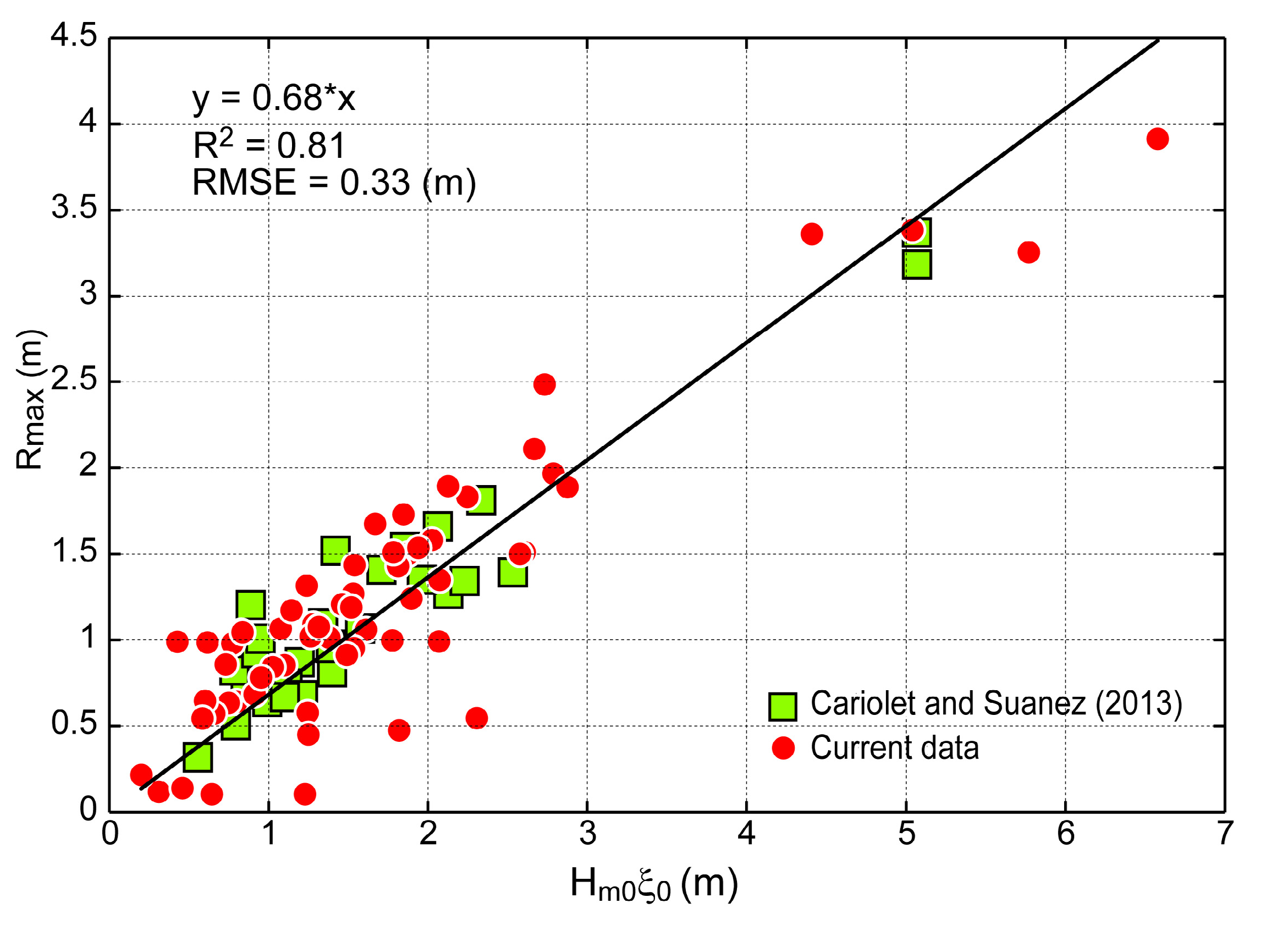
In comparison to the previous study of Cariolet and Suanez, the use of observed water level changes due to astronomical tide and/or storm surges for the calculation of beach slope gives better results (RMSE decreasing from 0.33 to 0.29 m for Equations (8) and (10), respectively). This is explained by the fact that both the upper and lower bounds defining the beach section on which the slope is calculated are shifting according to the sea level changes. Therefore, the slope values obtained are much more fair and accurate, especially when the beach profile is concave and tidal range is large (≈7 m), as is the case in this study.

-

Taking into account the environmental conditions and dimensional swash parameters of the Vougot beach, the Stockdon’s Equations (4)–(6) [21] may also be used with the appropriate beach slope value β_ƒ.

-

Dune retreat, and hence volume of sand eroded, depends on extreme water level (and therefore the frequency and intensity of each runup event) when its height is greater than that the toe of the dune.

-

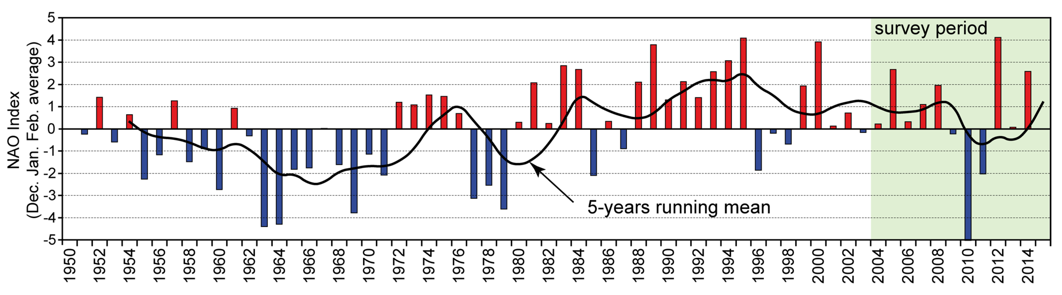
A good relationship seems to be revealed between erosion phases of the dune due to high extreme water levels and NAO+. In contrast, NAO− is associated to phases of dune recovery during cold and non-stormy winters.

References

1. Battjes, J.A. Run-up distributions of waves breaking on slopes. J. Waterw. Harb. Coast. Eng. Div. ASCE 1971, 97, 91–114. [Google Scholar]
2. Edelman, T.I. Dune erosion during storm conditions. In Proceedings of the 11th Conference on Coastal Engineering, London, UK, September 1968; pp. 719–722.
3. Van der Meulen, T.; Gourlay, M.R. Beach and dune erosion tests. In Proceedings of the 11th Conference on Coastal Engineering, London, UK, September 1968; pp. 701–707.
4. Edelman, T. Dune erosion during storm conditions. In Proceedings of the 13th Conference on Coastal Engineering, Vancouver, BC, Canada, 10–14 July 1972; pp. 1305–1311.
5. Van de Graaff, J. Dune erosion during a storm surge. Coast. Eng. 1977, 1, 99–134. [Google Scholar] [CrossRef]
6. Van de Graaff, J. Probabilistic design of dunes; an example from the Netherlands. Coast. Eng. 1986, 9, 479–500. [Google Scholar] [CrossRef]
7. Stockdon, H.F.; Sallenger, A.H.; Holman, R.A.; Howd, P.A. A simple model for the spatially-variable coastal response to hurricanes. Mar. Geol. 2007, 238, 1–20. [Google Scholar] [CrossRef]
8. Vellinga, P. Beach and dune erosion during storm surges. Coast. Eng. 1982, 6, 361–387. [Google Scholar] [CrossRef]
9. Fisher, J.S.; Overton, M.F. Numerical model for dune erosion due to wave uprush. In Proceedings of the 19th Coastal Engineering Conference, Houston, TX, USA, 3–7 September 1984; pp. 1553–1558.
10. Kriebel, D.L.; Dean, R.G. Numerical simulation of time-dependent beach and dune erosion. Coast. Eng. 1985, 9, 221–245. [Google Scholar] [CrossRef]
11. Kriebel, D.L. Verification study of a dune erosion model. Shore Beach 1986, 54, 13–21. [Google Scholar]
12. Overton, M.; Fisher, J.; Young, M. Laboratory Investigation of Dune Erosion. J. Waterw. Port. Coast. Ocean Eng. 1988, 114, 367–373. [Google Scholar] [CrossRef]
13. Carter, R.W.G.; Stone, G.W. Mechanisms associated with the erosion of sand dune cliffs, Magilligan, Northern Ireland. Earth Surf. Process. Landf. 1989, 14, 1–10. [Google Scholar] [CrossRef]
14. Pye, K.; Neal, A. Coastal dune erosion at Formby Point, north Merseyside, England: Causes and Mechanisms. Mar. Geol. 1994, 119, 39–56. [Google Scholar] [CrossRef]
15. Larson, M.; Erikson, L.; Hanson, H. An analytical model to predict dune erosion due to wave impact. Coast. Eng. 2004, 51, 675–696. [Google Scholar] [CrossRef]
16. Erikson, L.H.; Larson, M.; Hanson, H. Laboratory investigation of beach scarp and dune recession due to notching and subsequent failure. Mar. Geol. 2007, 245, 1–19. [Google Scholar] [CrossRef]
17. Claudino-Sales, V.; Wang, P.; Horwitz, M.H. Factors controlling the survival of coastal dunes during multiple hurricane impacts in 2004 and 2005: Santa Rosa barrier island, Florida. Geomorphology 2008, 95, 295–315. [Google Scholar] [CrossRef]
18. Sallenger, A.H. Storm impact scale for barrier islands. J. Coast. Res. 2000, 16, 890–895. [Google Scholar]
19. Ruggiero, P.; Komar, P.D.; McDougal, W.G.; Marra, J.J.; Beach, R.A. Wave runup, extreme water levels and erosion of properties backing beaches. J. Coast. Res. 2001, 17, 407–419. [Google Scholar]
20. Pye, K.; Blott, S.J. Decadal-scale variation in dune erosion and accretion rates: An investigation of the significance of changing storm tide frequency and magnitude on the Sefton coast, UK. Geomorphology 2008, 102, 652–666. [Google Scholar] [CrossRef]
21. Stockdon, H.F.; Holman, R.A.; Howd, P.A.; Sallenger, A.H. Empirical parameterization of setup, swash, and runup. Coast. Eng. 2006, 53, 573–588. [Google Scholar] [CrossRef]
22. Wassing, F. Model Investigation on Wave Run-Up Carried Out in the Netherland during the Past Twenty Years; Amer. Soc. Civil Engrs: Gainesville, FL, USA, 1957; Volume 6, pp. 700–714. [Google Scholar]
23. Hunt, I.A. Design of seawalls and breakwaters. J. Waterw. Harb. Div. 1959, 85, 123–152. [Google Scholar]
24. Guza, R.T.; Thornton, E.B. Swash oscillations on a natural beach. J. Geophys. Res. Ocean. 1982, 87, 483–491. [Google Scholar] [CrossRef]
25. Holman, R.A. Extreme value statistics for wave run-up on a natural beach. Coast. Eng. 1986, 9, 527–544. [Google Scholar] [CrossRef]
26. Longuet-Higgins, M.S.; Stewart, R.W. Radiation stress and mass transport in gravity waves, with application to. J. Fluid Mech. 1962, 13, 481–504. [Google Scholar] [CrossRef]
27. Battjes, J.A. Surf similarity. In Proceedings of the 14th Conference on Coastal Engineering, Copenhagen, Denmark, 24–28 June 1974; pp. 466–480.
28. Holman, R.A.; Sallenger, A.H. Setup and swash on a natural beach. J. Geophys. Res. Ocean 1985, 90, 945–953. [Google Scholar] [CrossRef]
29. Ruessink, B.G.; Kleinhans, M.G.; van den Beukel, P.G.L. Observations of swash under highly dissipative conditions. J. Geophys. Res. 1998, 103, 3111–3118. [Google Scholar] [CrossRef]
30. Ruggiero, P.; Holman, R.A.; Beach, R.A. Wave run-up on a high-energy dissipative beach. J. Geophys. Res. Ocean. 2004, 109. [Google Scholar] [CrossRef]
31. Mase, H. Random Wave Runup Height on Gentle Slope. J. Waterw. Port Coast. Ocean Eng. 1989, 115, 649–661. [Google Scholar] [CrossRef]
32. Nielsen, P.; Hanslow, D.J. Wave Runup Distributions on Natural Beaches. J. Coast. Res. 1991, 7, 1139–1152. [Google Scholar]
33. Cariolet, J.-M.; Suanez, S. Runup estimations on a macrotidal sandy beach. Coast. Eng. 2013, 74, 11–18. [Google Scholar] [CrossRef]
34. Guilcher, A.; Hallégouët, B. Coastal Dunes in Brittany and Their Management. J. Coast. Res. 1991, 7, 517–533. [Google Scholar]
35. Suanez, S.; Cariolet, J.-M.; Fichaut, B. Monitoring of recent morphological changes of the dune of Vougot beach (Brittany, France) using differential GPS. Shore Beach 2010, 78, 37–47. [Google Scholar]
36. Suanez, S.; Cariolet, J.-M. L’action des tempêtes sur l’érosion des dunes : Les enseignements de la tempête du 10 mars 2008. Norois 2010, 215, 77–99. [Google Scholar] [CrossRef] [Green Version]
37. Suanez, S.; Cariolet, J.-M.; Cancouët, R.; Ardhuin, F.; Delacourt, C. Dune recovery after storm erosion on a high-energy beach: Vougot Beach, Brittany (France). Geomorphology 2012, 139–140, 16–33. [Google Scholar] [CrossRef]
38. Blaise, E.; Suanez, S.; Stéphan, P.; Fichaut, B.; David, L.; Cuq, V.; Autret, R.; Houron, J.; Rouan, M.; Floc’h, F.; et al. Bilan des tempêtes de l’hiver 2013–2014 sur la dynamique de recul du trait de côte en Bretagne. Géomorphol. Relief Process. Environ. 2015, in press. [Google Scholar]
39. Senechal, N.; Coco, G.; Bryan, K.R.; Holman, R.A. Wave runup during extreme storm conditions. J. Geophys. Res. Ocean 2011, 116. [Google Scholar] [CrossRef]
40. Rascle, N.; Ardhuin, F. A global wave parameter database for geophysical applications. Part 2: Model validation with improved source term parameterization. Ocean Model. 2013, 70, 174–188. [Google Scholar] [CrossRef]
41. Roland, A.; Ardhuin, F. On the developments of spectral wave models: Numerics and parameterizations for the coastal ocean. Ocean Dyn. 2014, 64, 833–846. [Google Scholar] [CrossRef]
42. De Bakker, A.T.M.; Tissier, M.F.S.; Ruessink, B.G. Shoreline dissipation of infragravity waves. Cont. Shelf Res. 2014, 72, 73–82. [Google Scholar] [CrossRef]
43. Mayer, R.H.; Kriebel, D.L. Wave runup on composite-slope and concave beaches. In Proceedings of the 24th Coastal Engineering Conference, ASCE, Kobe, Japan, 23–28 October 1994; pp. 2325–2339.
44. McCallum, E.; Norris, W.J.T. The storms of January and February 1990. Meteorol. Mag. 1990, 119, 201–210. [Google Scholar]
45. Betts, N.L.; Orford, J.D.; White, D.; Graham, C.J. Storminess and surges in the South-Western Approaches of the eastern North Atlantic: The synoptic climatology of recent extreme coastal storms. Mar. Geol. 2004, 210, 227–246. [Google Scholar] [CrossRef]
46. Castelle, B.; Marieu, V.; Bujan, S.; Splinter, K.D.; Robinet, A.; Sénéchal, N.; Ferreira, S. Impact of the winter 2013–2014 series of severe Western Europe storms on a double-barred sandy coast: Beach and dune erosion and megacusp embayments. Geomorphology 2015, 238, 135–148. [Google Scholar] [CrossRef]
47. NOAA’s Climate Prediction Center Home Page. Available online: http://www.cpc.ncep.noaa.gov (accessed on 7 February 2015).
48. Masselink, G.; Austin, M.; Scott, T.; Poate, T.; Russell, P. Role of wave forcing, storms and NAO in outer bar dynamics on a high-energy, macro-tidal beach. Geomorphology 2014, 226, 76–93. [Google Scholar] [CrossRef]
49. Thomas, T.; Phillips, M.R.; Williams, A.T. Mesoscale evolution of a headland bay: Beach rotation processes. Geomorphology 2010, 123, 129–141. [Google Scholar] [CrossRef]
50. Thomas, T.; Phillips, M.R.; Williams, A.T.; Jenkins, R.E. Medium timescale beach rotation; gale climate and offshore island influences. Geomorphology 2011, 135, 97–107. [Google Scholar] [CrossRef]
51. O’Connor, M.C.; Cooper, J.A.G.; Jackson, D.W.T. Decadal Behavior of Tidal Inlet-Associated Beach Systems, Northwest Ireland, in Relation to Climate Forcing. J. Sediment. Res. 2011, 81, 38–51. [Google Scholar] [CrossRef]
52. Vespremeanu-Stroe, A.; Constantinescu, S.; Tatui, F.; Giosan, L. Multi-decadal Evolution and North Atlantic Oscillation Influences on the Dynamics of the Danube Delta Shoreline. J. Coast. Res. 2007, 2007, 157–162. [Google Scholar]
53. Montreuil, A.-L.; Bullard, J.E. A 150-year record of coastline dynamics within a sediment cell: Eastern England. Geomorphology 2012, 179, 168–185. [Google Scholar] [CrossRef] [Green Version]