A Programmable Aerial Multispectral Camera System for In-Season Crop Biomass and Nitrogen Content Estimation

Abstract

The study introduces a prototype multispectral camera system for aerial estimation of above-ground biomass and nitrogen (N) content in winter wheat (Triticum aestivum L.). The system is fully programmable and designed as a lightweight payload for unmanned aircraft systems (UAS). It is based on an industrial multi-sensor camera and a customizable image processing routine. The system was tested in a split fertilized N field trial at different growth stages in between the end of stem elongation and the end of anthesis. The acquired multispectral images were processed to normalized difference vegetation index (NDVI) and red-edge inflection point (REIP) orthoimages for an analysis with simple linear regression models. The best results for the estimation of above-ground biomass were achieved with the NDVI (R${}^2$ = 0.72–0.85, RMSE = 12.3%–17.6%), whereas N content was estimated best with the REIP (R${}^2$ = 0.58–0.89, RMSE = 7.6%–11.7%). Moreover, NDVI and REIP predicted grain yield at a high level of accuracy (R${}^2$ = 0.89–0.94, RMSE = 9.0%–12.1%). Grain protein content could be predicted best with the REIP (R${}^2$ = 0.76–0.86, RMSE = 3.6%–4.7%), with the limitation of prediction inaccuracies for N-deficient canopies.

1. Introduction

Extensive use of nitrogen (N) leads to negative environmental impacts, like eutrophication, acid rains, drinking water contamination and nitrous oxide emissions [1,2,3,4,5]. Nevertheless, N plays a major role in crop growth and crop quality in wheat (Triticum L.) production [6]. Farmers have to achieve a certain quantity and quality of yield. Thus, they require N fertilization strategies that may ensure good outcomes for both yields and the environment. The calculation of appropriate amounts of N and the correct timing of the fertilization are crucial to supply the crop with sufficient nutrients at all stages of crop development. Moreover, it decreases the risk of N loss through leaching [7] and nitrous oxide emissions [8].

In wheat cultivation, split N application is a common way to influence grain yield and grain protein content. Several studies have shown that N applications before flowering increase mainly grain mass [9], whereas N applications around flowering increase mainly grain protein content [10,11]. In the past, farmers often used simplified methods to estimate the N demand for late N applications. Nowadays, rules of thumb like 1 kg N per 1000 kg of expected grain yield are more and more replaced by methods that take soil available N, previous N applications, above-ground biomass and its current N content into account [12,13]. A common N recommendation method is to measure the N content in plant leaves during the vegetative period and to compare it to a critical amount of N, required for a maximum of biomass production [14,15,16]. The critical N content in winter wheat (Triticum aestivum L.) was defined by Justes et al. [17,18] in a universal equation based on the actual above-ground biomass. Thus, recommended rates can be calculated from actual estimates of biomass and N content alone.

As sampling of a representative amount of probes in a heterogeneous field is a costly and time-consuming task, farmers increasingly utilize online systems to collect site-specific information, to calculate appropriate amounts of fertilizer and to apply the dressing at the same time [19]. Most of these systems are based on optical sensors, which measure the plant canopy reflection to calculate targeted N prescription with a proprietary algorithm, e.g., the Yara N-Sensor (Yara International ASA, Oslo, Norway), the ISARIA crop sensor (Fritzmeier GmbH & Co. KG, Großhelfendorf, Germany) and the GreenSeeker (Trimble Navigation Ltd., Sunnyvale, CA, USA).

Within the last few years, remote sensing with unmanned aerial vehicles (UAVs) or unmanned aircraft systems (UASs) became popular in the precision agriculture domain. These systems are able to provide data at high spatial and temporal resolutions for crop and soil monitoring [20]. Commonly, researchers utilize image-based systems in the visual and near-infrared radiation spectrum [21], giving a more comprehensive impression of the field than spot measurements with ground-based detection systems. Aasen et al. [22] gave a detailed overview and definition of the different types of imaging systems, which are currently in use on-board UAVs. Generally, imaging systems can be classified as multispectral systems with few bands [23,24,25,26] and as more sophisticated hyperspectral systems with a multitude of bands [22,27,28]. The hyperspectral systems combine the benefits of high spectral and spatial resolution, but are still rare and expensive.

Above-ground biomass and N content of wheat are known to be detectable with a limited number of bands [16,29,30]. Therefore, this study focuses on the development of a multispectral camera system capable of estimating parameters for the calculation of optimal N applications. The system is intended to operate on-board a UAS, to be lightweight and fully programmable for future applications. To ensure operability in this context, the system was tested in a split fertilized N field trial in winter wheat before and after the late N application.

2. Materials and Methods

The camera system was designed as a lightweight payload for a UAS (see Figure 1a). It is based on an industrial multi-sensor camera (D3, VRMagic GmbH, Mannheim, Germany), with four identical monochrome imaging sensors, four identical lens systems and four different bandpass filters (bk Interferenzoptik Elektronik GmbH, Nabburg, Germany) (see Figure 1b). It offers several hardware interfaces and was coupled to a luminosity sensor to measure ambient solar radiation for exposure time calculation. Moreover, it was connected to the UAS’s processing unit via Ethernet connection. The specifications of all camera system components are given in Table 1.

The camera system is able to measure four narrow wavelength bands in the so-called red-edge region, a transition zone in between the visual and the near-infrared radiation spectrum, which is sensitive to leaf chlorophyll content [31,32,33]. For this study, the wavelength bands at 670, 700, 740 and 780 nm were selected. They can be used to approximate the normalized difference vegetation index (NDVI) [34] and the red-edge inflection point (REIP) [33]. The formulas are given in Equations (1) and (2), with $R_{nm}$ being the reflectance at the four narrow bands.

$$NDVI=\frac{(R_{780}-R_{670})}{(R_{780}+R_{670})}$$

(1)

$$REIP=700+40\times \frac{(\frac{(R_{670}+R_{780})}{2}-R_{700})}{(R_{740}-R_{700})}$$

(2)

Figure 1. Carrier platform “Hexe” (a) with the mounted VRMagic D3 camera system and four attached Aptina imaging sensors (b). The five main steps of the image acquisition and processing loop (c): (i) exposure time measurement; (ii) simultaneous image acquisition; (iii) vignetting correction; (iv) lens distortion correction; and (v) image-to-image registration.

Figure 1. Carrier platform “Hexe” (a) with the mounted VRMagic D3 camera system and four attached Aptina imaging sensors (b). The five main steps of the image acquisition and processing loop (c): (i) exposure time measurement; (ii) simultaneous image acquisition; (iii) vignetting correction; (iv) lens distortion correction; and (v) image-to-image registration.

Table 1. Overview of the camera system specifications. The system consists of an industrial D3 camera platform, four identical imaging sensors and lens systems, four specific bandpass filters and a luminosity sensor to measure ambient solar radiation.

Component	Parameter	Value	Parameter	Value
D3 platform	Name	VRmD3MFC
	CPU	1-GHz ARM Cortex-A8 Core	Memory	32 GB flash
	DSP	700-MHz C674x	RAM	2 GB DDR3-800
Image sensor	Name	Aptina MT9V024
	Size	4.51 mm (H) × 2.88 mm (V)	Pixel size	6 μm × 6 μm
	Resolution	752 px (H) × 480 px (V)	Shutter	Global
	Dynamic range	10 bit (1024)	Quantum eff.	~49%, 47.5%, 44%, 41%
	Type	CMOS monochrome (1/3 in)		(670, 700, 740, 780 nm)
Lens system	Focal length	3.6 mm	F-number	1.8
Filter	Type	Bandpass interference filter
	Wavelengths	670, 700, 740, 780 nm	Tmax	≥70, typically 85%
	Center	±2 nm	FWHM	10 ±2 nm
Luminosity	Name	TSL 2561
	Sensitivity	~350–900 nm	Dynamic range	0.1–40,000 lx

Table 1. Overview of the camera system specifications. The system consists of an industrial D3 camera platform, four identical imaging sensors and lens systems, four specific bandpass filters and a luminosity sensor to measure ambient solar radiation.

Component	Parameter	Value	Parameter	Value
D3 platform	Name	VRmD3MFC
	CPU	1-GHz ARM Cortex-A8 Core	Memory	32 GB flash
	DSP	700-MHz C674x	RAM	2 GB DDR3-800
Image sensor	Name	Aptina MT9V024
	Size	4.51 mm (H) × 2.88 mm (V)	Pixel size	6 μm × 6 μm
	Resolution	752 px (H) × 480 px (V)	Shutter	Global
	Dynamic range	10 bit (1024)	Quantum eff.	~49%, 47.5%, 44%, 41%
	Type	CMOS monochrome (1/3 in)		(670, 700, 740, 780 nm)
Lens system	Focal length	3.6 mm	F-number	1.8
Filter	Type	Bandpass interference filter
	Wavelengths	670, 700, 740, 780 nm	Tmax	≥70, typically 85%
	Center	±2 nm	FWHM	10 ±2 nm
Luminosity	Name	TSL 2561
	Sensitivity	~350–900 nm	Dynamic range	0.1–40,000 lx

Both NDVI and REIP are well-known measures for winter wheat properties, such as above-ground biomass, N content and grain yield. The REIP is commonly used to estimate crop N content, whereas the NDVI is often used for biomass estimation and grain yield prediction [16,30].

2.1. Image Acquisition Loop

The camera system is fully programmable and was operated with an image acquisition and processing routine of five main steps (see Figure 1c): (i) the ambient solar radiation is detected by the luminosity sensor and processed to an optimal exposure time; (ii) four individual images are acquired simultaneously and saved to the flash memory; (iii) a vignetting correction is applied to each image for the compensation of brightness reduction at the image borders; (iv) the lens distortion error is corrected by re-sampling each image to a rectilinear projection; and (v) the four images are spatially co-registered by a perspective transformation. Steps (i) and (ii) are always performed on-board the camera, whereas Steps (iii)–(v) can be performed on-board or in post-processing.

2.1.1. Exposure Time

The exposure time is an important parameter for an imaging system. It controls the shutter and, as a consequence, the amount of time the imaging sensor is exposed to electro-magnetic radiation. Finding an optimal exposure time prevents the sensor from under- and over-exposure and allows one to make use of the sensor’s full dynamic range. As ambient solar radiation typically changes during a flight mission, the exposure time needs to be adjusted according to these changes. Therefore, the camera system was set up with a TSL 2561 luminosity sensor (Adafruit Industries, New York, NY, USA) to detect the changes on-the-fly (while flying). The sensor is equipped with two photo-diodes and is sensitive to the visible and near-infrared radiation spectrum (~350–900 nm). It is connected to the camera system via an i2c interface and read-out every time before image acquisition. To avoid angular effects of the radiation’s geometry, the sensor is covered with an ordinary ping-pong ball, which serves as a cosine corrector to diffuse the incoming radiation (see, i.e., Figure 2a).

Figure 2. Carrier platform “Hexe” with an attached TSL 2561 luminosity sensor, covered by a ping-pong ball, which serves as a radiation diffuser (a); exemplary histogram of a calibration image comprising soil, vegetation, bright and shadowed areas (b); exposure time calibration functions for each sensor/filter combination and the final mean exposure time calibration function (c).

Figure 2. Carrier platform “Hexe” with an attached TSL 2561 luminosity sensor, covered by a ping-pong ball, which serves as a radiation diffuser (a); exemplary histogram of a calibration image comprising soil, vegetation, bright and shadowed areas (b); exposure time calibration functions for each sensor/filter combination and the final mean exposure time calibration function (c).

To estimate optimal exposure time, several imagery sets were acquired under variable radiation conditions. The camera was set up on a platform 5 m above-ground and targeted towards two white and black reference targets in a scene comprising soil, vegetation, bright and shadowed areas, representing a typical surrounding for in-field operation. Images were acquired in an automatic loop, incrementing the exposure time from a fraction of a ms (under-exposure) to 10 ms (over-exposure). For each image, exposure time and luminosity sensor readings were saved for analysis. The procedure was performed from morning to evening during different days in late spring. The imagery sets were analyzed for their histogram stretch. Images without under- or over-exposure (clipping) and a spread of ≥60% of the 10-bit dynamic range were selected as valid (see Figure 2b). Approximately 2500 images were selected per band. Corresponding exposure times and luminosity readings were regressed for each band individually by a power function (see Figure 2c). All functions follow the same trend and increasingly converge for higher luminosity values. As bigger differences only appear at relatively dark ambient conditions, all functions were averaged to a mean exposure time function for all four sensor/filter combinations.

2.1.2. Sensitivity, Vignetting and Lens Distortion

After image acquisition, the images receive radiometric and geometric corrections, accounting for their specific sensor/filter/lens combination [35]. First, the images undergo two radiometric corrections: (i) compensation of the image sensor’s change in sensitivity at different wavelengths; and (ii) the correction of vignetting, the radial reduction of brightness towards the image borders [35]. Second, a geometric correction is performed to remove the rectilinear projection error, which is caused by the lens system [36]. All correction parameters are system constants and need to be determined only once or after system changes.

To reduce the effect of sensitivity on the radiometric intensity of all images, the sensors’ quantum efficiency ($Q{E}_{nm}$) values (see Table 1) were used to calculate correction factors for a radiometric normalization. In this setup, the sensor’s sensitivity is lowest in the near-infrared band ($Q{E}_{780}$ ~41%). This value was used as a reference for the calculation of the correction factors of all other images ($f_{QE}=Q{E}_{780}/Q{E}_{nm}$). In the acquisition loop, these factors are applied to the radiometric intensities of the images at 670, 700 and 740 nm before performing the vignetting correction. In order to quantify the effect of vignetting, the brightness gradient from each image center to the borders was determined by capturing a white target with defined reflectivity (~99%). The images were acquired on a cloudy day under the assumption of diffuse light conditions. The radiometric intensities of these reference images were, again, normalized to the mean reflection in the image and then inversed to create a correction factor matrix for each band. The matrices are applied to the captured images as a second radiometric correction. This correction does not only account for vignetting effects, but also for flaws of the sensor, lens and filter [35]. In the next step, the geometric distortion, deriving from the lens system, is corrected. Lens systems typically cause rectilinear projection errors, which need to be removed to preserve linear objects as straight lines [36]. Therefore, the parameters of distortion were estimated by camera calibration with the software Agisoft Lens 0.4.1 (Agisoft LLC, St. Petersburg, RU). These parameters are used to re-sample the images to a rectilinear projection as a first geometric correction.

2.1.3. Image-To-Image Registration

In the last step, the four individual images are geometrically aligned, cropped to a common extent and stacked to a multi-layered image. The implemented image-to-image registration procedure utilizes a perspective transformation to re-sample the images into a common coordinate system [37]. The transformation and cropping parameters were determined experimentally. The camera system was triggered at altitudes of 10 and 20 m above a sports ground facing a pattern of lines. The captured images were corrected for the lens distortion effects and, consequently, manually registered to identify the transformation parameters for image-to-image registration and cropping. As the optical axes of the lens systems were not aligned perfectly parallel, the parameters of projection vary for different distances [37]. As a consequence, the results of the manual registration were used to create a function of distance to calculate the parameters for any flight altitude, assuming a nadir view. The registration, therefore, depends on a measure of distance, which is provided as flight altitude by the UAS’s control unit.

2.2. Carrier Platform

The camera system was installed on “Hexe”, a modified MikroKopter (HiSystems GmbH, Moormerland, Germany) Hexa XL aerial carrier platform (see Figure 1a). “Hexe” is an unmanned aircraft system with standard multi-copter navigation capabilities. It is equipped with an inertial measurement unit (IMU) and a differential global navigation satellite system (GNSS) receiver. Moreover, it features an additional accelerometer to improve altitude accuracy. It can be assembled with a payload of ~1 kg and is powered by a 5000 mAh lithium polymer battery for an operation time of approximately 10 min. “Hexe” offers on-board sensor control and sensor data processing by a software framework, running on a Raspberry Pi 1 Model B single-board computer (Raspberry Pi Foundation, Caldecote, UK). The framework retrieves the navigation data and all sensor measurements for on-board data fusion, logging and broadcasting [38]. It shares the navigation information, i.e., the altitude, with the attached camera system. In addition to the multispectral camera system, “Hexe” was equipped with a simple RGB camera with a resolution of 2592 × 1944 pixels (Raspberry Pi Foundation, Caldecote, UK). Both systems were installed on a roll- and pitch-stabilized gimbal to ensure a best-possible nadir view.

2.3. Field Trial

The camera system was tested on a field trial, established at the Ihinger Hof (48.74${}^{\circ }$ N, 8.92${}^{\circ }$ E), a research station of the University of Hohenheim. The region has a temperate climate with an annual average temperature of 7.9 ${}^{\circ }$C and an average precipitation of 690 mm. This season had 1266 growing degree days with an average winter temperature of 3.3 ${}^{\circ }$C and an average summer temperature of 16.0 ${}^{\circ }$C. The field trial was laid out on silty clay soil, comprising an area of 840 m${}^2$. One cultivar of winter wheat (“Pamier”) was treated with seven N fertilization levels of 0, 4, 8, 12, 16, 20 and 24 g·m${}^{-2}$ in a randomized complete block design with three replicates. Figure 3 gives an overview of the 21 plots, each of a size of 10 × 4 m. The total amount of N was split into three dressings and applied at growth stages Z 20, Z 31 and Z 51 (see Table 2) [39]. The growth stages correspond to the beginning of tillering, the beginning of stem elongation and the beginning of ear emergence, respectively. An analysis of soil N before the first dressing showed a uniform level of 1.6 g·m${}^{-2}$ for all plots. Plant protection followed common practice.

Figure 3. N field trial in winter wheat with 21 plots of a size of 10 × 4 m each. Seven N fertilization levels of 0, 4, 8, 12, 16, 20 and 24 g·m${}^{-2}$ were tested in a randomized complete block design with three replicates.

Figure 3. N field trial in winter wheat with 21 plots of a size of 10 × 4 m each. Seven N fertilization levels of 0, 4, 8, 12, 16, 20 and 24 g·m${}^{-2}$ were tested in a randomized complete block design with three replicates.

Table 2. Overview of the applied N dressings for each treatment (N${}_x$) at different growth stages (Z) and the accumulated precipitation (P) since the last dressing.

Date	Z	N${}_0$	N${}_4$	N${}_8$	N${}_{12}$ (g·m${}^{-2}$)	N${}_{16}$	N${}_{20}$	N${}_{24}$	P (mm·m${}^{-2}$)
20 March 2015	20	0	2	3	4	6	8	10
24 April 2015	31	0	2	3	4	6	8	10	43.8
26 May 2015	39–41								70.7
2 June 2015	51								79.7
5 June 2015	51	0	0	2	4	4	4	4	79.7
10 June 2015	61								46.0
17 June 2015	69								46.4
5 August 2015	90								104.3

Table 2. Overview of the applied N dressings for each treatment (N${}_x$) at different growth stages (Z) and the accumulated precipitation (P) since the last dressing.

Date	Z	N${}_0$	N${}_4$	N${}_8$	N${}_{12}$ (g·m${}^{-2}$)	N${}_{16}$	N${}_{20}$	N${}_{24}$	P (mm·m${}^{-2}$)
20 March 2015	20	0	2	3	4	6	8	10
24 April 2015	31	0	2	3	4	6	8	10	43.8
26 May 2015	39–41								70.7
2 June 2015	51								79.7
5 June 2015	51	0	0	2	4	4	4	4	79.7
10 June 2015	61								46.0
17 June 2015	69								46.4
5 August 2015	90								104.3

2.4. Measurements

Four flight missions were performed during mid-season crop development. The missions were conducted 10 and 3 days before, as well as 5 and 12 days after the third N dressing (Z 39–41, Z 51, Z 61, Z 69). The growth stages correspond to the end of stem elongation, the beginning of ear emergence, the beginning of anthesis and the end of anthesis. The flight missions comprised the N field trial and an adjacent field trial, covering a total area of approximately 2500 m${}^2$. The adjacent field trial is not part of this study. The white reference target was laid out beside the plots. Aerial images were acquired at a scheduled flight altitude of 25 m, a forward lap of 95%, a side lap of 60% and a desired ground resolution of 0.04 m·px${}^{-1}$. The azimuthal orientation at image acquisition was constant during the missions (~320${}^{\circ }$). The image processing loop (see Figure 1c) was performed during flight, which resulted in an acquisition rate of approximately 0.25 Hz. Six ground control points were measured with a real-time kinematic GNSS receiver (Trimble Navigation Ltd., Sunnyvale, CA, USA). Table 3 gives an overview of all mission parameters.

Table 3. Overview of the performed flight missions at different growth stages (Z). The table comprises the mission date, the number of images (n) for subsequent processing, the scheduled flight altitude (A), the number of ground control points (G), the desired image ground resolution (R), the mission time (T), the weather conditions (W), the solar zenith (Ze) and azimuth angle (Az) and the wind speed (S).

Date	Z	n	A (m)	G	R (m·px${}^{-1}$)	T	W	Ze ${(}^{°})$	Az ${(}^{°})$	S (m·s${}^{-1}$)
26 May 2015	39–41	121	25	6	0.04	10–11 a.m.	clear sky	44	114	2
2 June 2015	51	128	25	6	0.04	10–11 a.m.	clear sky	43	113	3
10 June 2015	61	132	25	6	0.04	2–3 p.m.	clear sky	29	212	2
17 June 2015	69	135	25	6	0.04	2–3 p.m.	clear sky	29	212	1

Table 3. Overview of the performed flight missions at different growth stages (Z). The table comprises the mission date, the number of images (n) for subsequent processing, the scheduled flight altitude (A), the number of ground control points (G), the desired image ground resolution (R), the mission time (T), the weather conditions (W), the solar zenith (Ze) and azimuth angle (Az) and the wind speed (S).

Date	Z	n	A (m)	G	R (m·px${}^{-1}$)	T	W	Ze ${(}^{°})$	Az ${(}^{°})$	S (m·s${}^{-1}$)
26 May 2015	39–41	121	25	6	0.04	10–11 a.m.	clear sky	44	114	2
2 June 2015	51	128	25	6	0.04	10–11 a.m.	clear sky	43	113	3
10 June 2015	61	132	25	6	0.04	2–3 p.m.	clear sky	29	212	2
17 June 2015	69	135	25	6	0.04	2–3 p.m.	clear sky	29	212	1

After every mission, ground-truth information was acquired by destructive sampling of above-ground biomass in an area of 0.6 m${}^2$ per plot. The crops were cut as close to the soil surface as possible, and fresh matter was determined. Probes of the samples were dried to constant mass in a drying cabinet at 80 ${}^{\circ }$C and analyzed for dry matter (DM) and N content. N content was determined by near-infrared spectroscopy (NIRS XDS, FOSS, DK). Harvest took place on 5 August 2015. Again, each plot was sampled in the same way as after the flight missions. The samples were analyzed for grain yield and N content. Grain protein content was derived by multiplication of the N content with a universal conversion factor of 6.25.

2.5. Image Processing

The images were processed to multispectral orthoimages, using the 3D reconstruction software Agisoft PhotoScan Professional Edition 1.1.6 (Agisoft LLC, St. Petersburg, Russia). The images, the ground control point coordinates and the flight log, containing the coarse image locations, were imported. After the first step of coarse alignment, manual identification of the ground control points was performed to optimize the alignment procedure. In the next step, the 3D scene was reconstructed as a point cloud and triangulated to build a digital elevation model. In the last step, the images were mosaicked to an orthoimage and exported in the GeoTIFF format (WGS84/UTM32N) for each flight mission, individually. The mosaicking method followed the description of Bendig et al. [40] utilizing the radiometric information from the best centered image in case of overlap. Color correction was not performed.

Further processing was conducted with the statistical computation software R [41], making use of the “spatial” and “raster” packages [42,43]. The radiometric intensities at the position of the white reflection target were used to compute averaged normalization factors for the four bands. Subsequently, all bands were normalized with these factors to transform the radiometric intensities into reflectance values. According to Equations (1) and (2), the NDVI and REIP layer were calculated for each orthoimage. The field trial’s plot information was imported as polygonal shapefile. Each plot was reduced to a size of 6 × 1 m to account for plot boundary effects (e.g., inaccuracies in fertilization) and for excluding the reference sample areas from analysis (see Figure 3). Consequently, a spatial query was performed to extract the NDVI and REIP values of the raster cells, which fall inside a polygon. For each polygon, a summary statistics was calculated to average the values of the NDVI and the REIP.

2.6. Regression Analysis

In the last step of processing, a simple linear regression analysis was carried out to confirm the multispectral camera system’s ability to detect and predict certain parameters of interest. The analysis was split into two parts: (i) a regression analysis to infer the sampled information at each flight mission; and (ii) a regression analysis to predict the sampled information at harvest (Z 90). The averaged NDVI and REIP values served as independent variable. They were used to estimate above-ground biomass and N content, as well as to predict grain yield and grain protein content. The models were evaluated by comparison of the coefficients of determination (R${}^2$), the root mean square error (RMSE), the relative RMSE and the bias. The quality of each model was assessed by leave-one-out cross-validation and the resulting root mean square error of validation (RMSEV).

3. Results

The on-board camera system was able to capture multispectral images for all UAS flight missions. Reference samples were taken and analyzed to ensure the comparison to real ground truth data. The regression analyses indicate valuable first results.

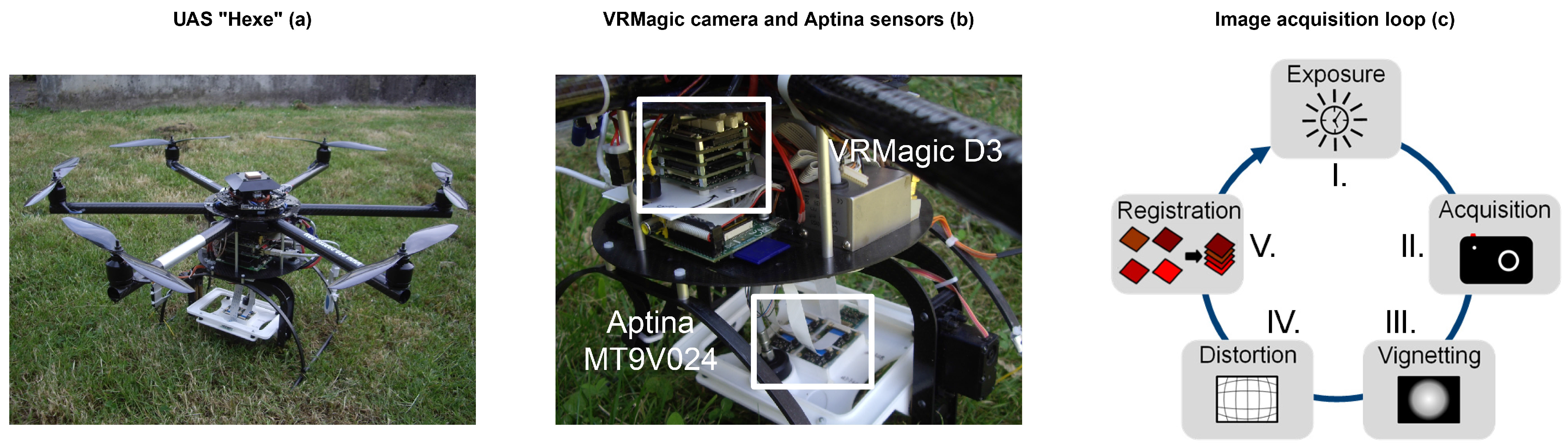
3.1. Image Acquisition Loop

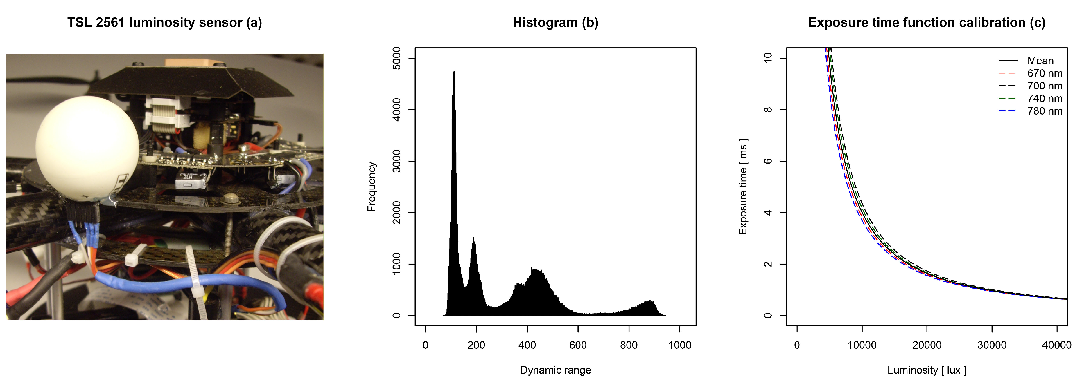
The camera system worked as expected. It performed all steps of the acquisition loop during the flight mission. One iteration, comprising the steps from exposure time definition to image-to-image registration, took approximately 4 s of time. The exposure time function led to an acquisition of images with a contrast stretch ≥60% of the 10-bit dynamic range. Due to the approximated mean exposure time function, some images had clipping effects at the white reference target.

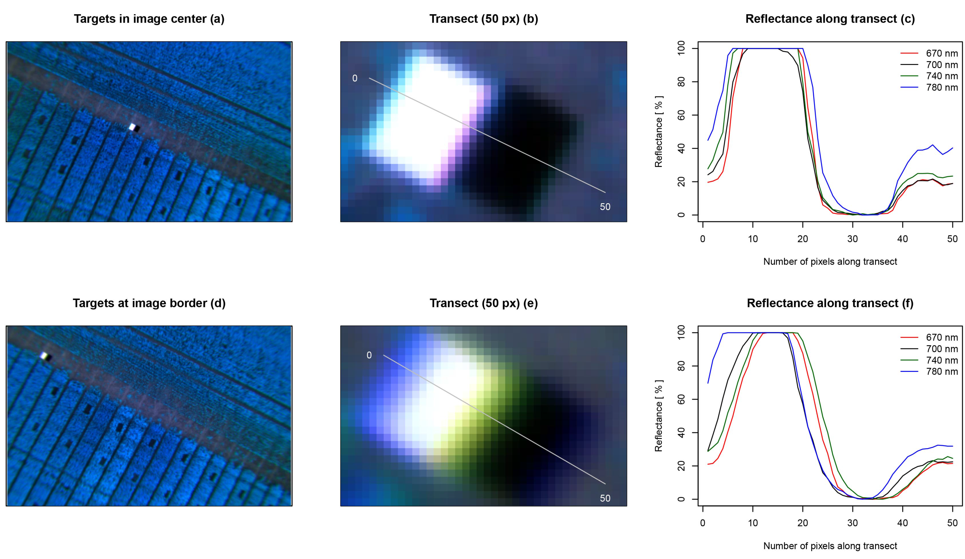
Registered multispectral images were cropped to a common extent of 732 × 464 px and showed a geometrical error in alignment accuracy (see Figure 4). The error was unevenly distributed throughout the image. Objects that were near the image’s center showed a smaller displacement in alignment (~2 px), whereas objects at the image’s border showed a larger displacement (~6 px).

Figure 4. Image-to-image registration accuracy at different locations within the image. Two registered multispectral images are presented as false color images. The first image sets focus on two black and white reference targets (a); whereas the second image captures the targets at its border (d); two transects of a length of 50 px were selected to investigate the spatial displacement of the four registered bands (b,e); the reflectance along the transects is shown on the right. The spatial displacement can be observed on the x-axis, and the reflectance can be observed on the y-axis. The figures indicate that the spatial alignment is better in the center of an image (~2 px) (c); and it is worse in the border region (~6 px) (f).

Figure 4. Image-to-image registration accuracy at different locations within the image. Two registered multispectral images are presented as false color images. The first image sets focus on two black and white reference targets (a); whereas the second image captures the targets at its border (d); two transects of a length of 50 px were selected to investigate the spatial displacement of the four registered bands (b,e); the reflectance along the transects is shown on the right. The spatial displacement can be observed on the x-axis, and the reflectance can be observed on the y-axis. The figures indicate that the spatial alignment is better in the center of an image (~2 px) (c); and it is worse in the border region (~6 px) (f).

3.2. Measurements

The laboratory analysis of the samples from Z 39–41 to Z 69 are presented in Table 4. Due to an error in the procedure, one sample could not be analyzed for Z 51 and Z 69, respectively. Average biomass showed an increase from 381.8–1351.3 g·m${}^{-2}$ over time. Mean N content was stable at Z 39–41 and Z 51 (1.5 g 100 g${}^{-1}$), decreased at Z 61 (1.2 g 100 g${}^{-1}$) and increased slightly at Z 69 (1.3 g 100 g${}^{-1}$).

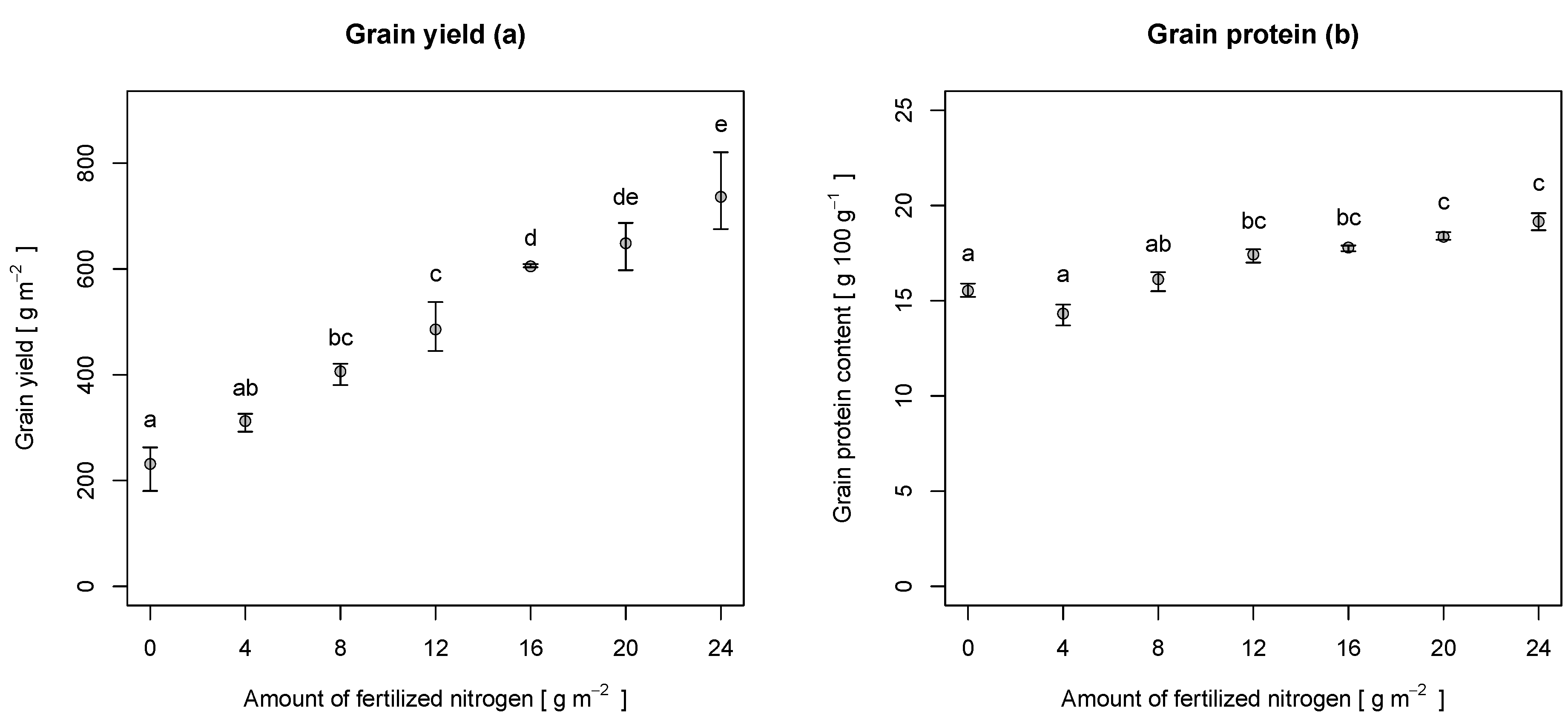
Table 4 also shows the results of the samples at harvest (Z 90). Grain yield ranged from 180.4–820.7 g·m${}^{-2}$. The yield increased almost linearly with the amount of fertilized N (see Figure 5a). Grain protein content ranged from 13.7–19.6 g 100 g${}^{-1}$. The protein content did not increase linearly with the amount of fertilized N (see Figure 5b). Its minimum was at an N level of 4 g·m${}^{-2}$, whereas its maximum was reached at a level of 24 g·m${}^{-2}$.

Table 4. Descriptive statistics (minimum, mean, maximum and standard deviation (SD)) of above-ground biomass, N content, grain yield and grain protein content, sampled at different growth stages (Z).

Variable	Z	Minimum	Mean	Maximum	SD
Biomass (DM) (g·m${}^{-2}$)	39–41	91.9	381.8	665.5	130.13
	51	241.8	512.1	848.0	165.17
	61	444.4	955.5	1447.3	324.26
	69	486.1	1351.3	2076.0	432.97
N content (g 100 g${}^{-1}$)	39–41	1.1	1.5	2.0	0.30
	51	1.1	1.5	2.2	0.36
	61	0.9	1.2	1.9	0.28
	69	0.9	1.3	1.7	0.24
Grain yield (g·m${}^{-2}$)	90	180.4	489.7	820.7	178.74
Grain protein content (g 100 g${}^{-1}$)	90	13.7	17.0	19.6	1.65

Table 4. Descriptive statistics (minimum, mean, maximum and standard deviation (SD)) of above-ground biomass, N content, grain yield and grain protein content, sampled at different growth stages (Z).

Variable	Z	Minimum	Mean	Maximum	SD
Biomass (DM) (g·m${}^{-2}$)	39–41	91.9	381.8	665.5	130.13
	51	241.8	512.1	848.0	165.17
	61	444.4	955.5	1447.3	324.26
	69	486.1	1351.3	2076.0	432.97
N content (g 100 g${}^{-1}$)	39–41	1.1	1.5	2.0	0.30
	51	1.1	1.5	2.2	0.36
	61	0.9	1.2	1.9	0.28
	69	0.9	1.3	1.7	0.24
Grain yield (g·m${}^{-2}$)	90	180.4	489.7	820.7	178.74
Grain protein content (g 100 g${}^{-1}$)	90	13.7	17.0	19.6	1.65

Figure 5. Grain yield (a) and grain protein content (b) at different levels of fertilization, sampled at harvest (Z 90). The points represent the mean values, whereas the whiskers represent the minima and maxima. Letters indicate the results of a Tukey’s HSD multiple comparison test ($\alpha =0.05$).

Figure 5. Grain yield (a) and grain protein content (b) at different levels of fertilization, sampled at harvest (Z 90). The points represent the mean values, whereas the whiskers represent the minima and maxima. Letters indicate the results of a Tukey’s HSD multiple comparison test ($\alpha =0.05$).

3.3. Image Processing

An orthoimage was computed from the acquired aerial imagery for each growth stage. The resulting RMSEs of the ground control point residuals ranged from 0.027–0.032 m in the horizontal and from 0.035–0.046 m in the vertical direction. The orthoimages were produced with a ground resolution of 0.04 m·px${}^{-1}$, leading to an analysis at the canopy level with mixed signals, comprising soil and plant reflection [44]. The signals were used to compute the NDVI and the REIP layer, which were analyzed for the selected plot areas (see Figure 6). At Z 39–61, the average NDVI values were constant around 0.79 with a standard deviation of 0.07 and decreased at Z 69 (0.68 ± 0.10). The average REIP values were higher for Z 51 and Z 61 (~739 ± 4.2), whereas they were lower for Z 39–41 and Z 69 (~735 ± 4.7).

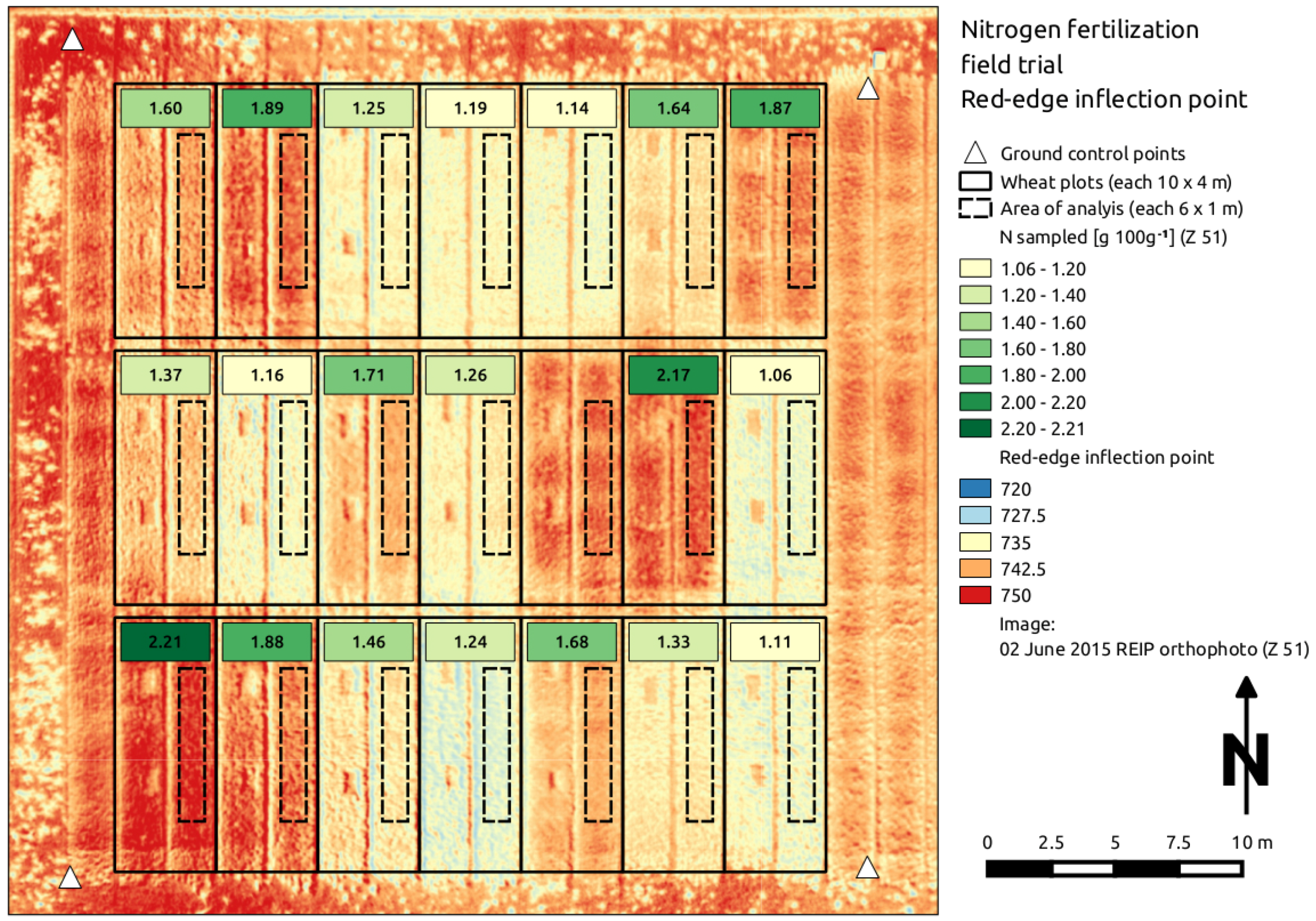
Figure 6. Exemplary red-edge inflection point (REIP) orthoimage with sampled above-ground biomass N content values (g 100 g${}^{-1}$) at growth stage Z 51. One sample is missing due to an erroneous laboratory analysis.

Figure 6. Exemplary red-edge inflection point (REIP) orthoimage with sampled above-ground biomass N content values (g 100 g${}^{-1}$) at growth stage Z 51. One sample is missing due to an erroneous laboratory analysis.

3.4. Regression Analysis

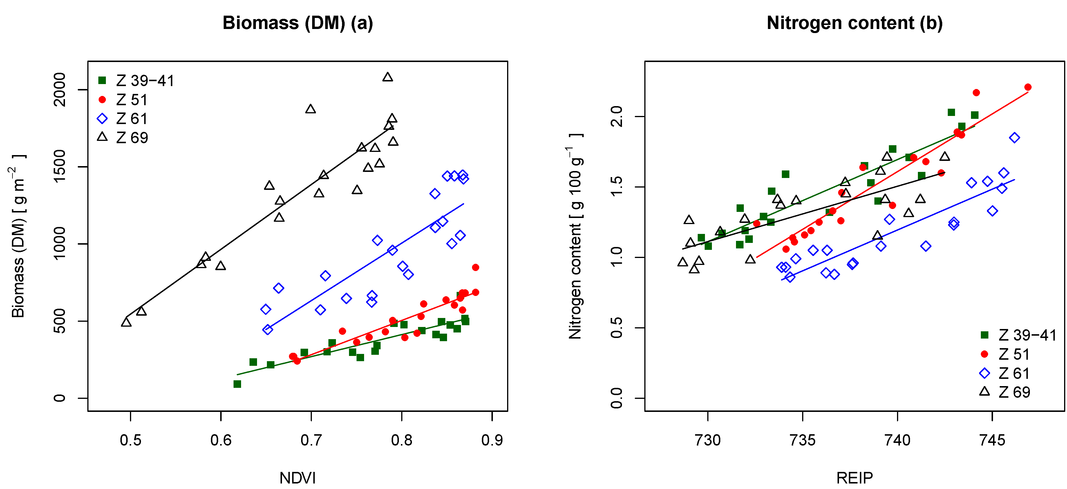
The regression results are grouped by the two aims of this analysis: (i) estimation of biomass and N content; and (ii) prediction of grain yield and grain protein content. All regressions were significant ($p<0.001$). Table 5 shows the results of the biomass and N content estimation. The table indicates that the NDVI performed better than the REIP. The NDVI estimated the biomass best at Z 39–41, Z 51 and Z 69 with coefficients of determination (R${}^2$) of 0.78, 0.85 and 0.84 and relative RMSE values of 15.7%, 12.3% and 12.3%. The REIP estimated the biomass best at Z 61 with an R${}^2$ of 0.77 and a relative RMSE of 15.8%. Figure 7a displays the regression lines for the NDVI at the different growth stages. The relationship between NDVI and biomass appeared to be linear for all growth stages, whereas the slopes of the regression lines increased with the gain in biomass over time.

For N content estimation, the REIP gave the best results. The R${}^2$ showed values of 0.83, 0.89, 0.81 and 0.58 with relative RMSE values of 8.3%, 7.6%, 10.3% and 11.7% (Z 39–69). The REIP performed best at growth stage Z 51 and worst at growth stage Z 69. The regression plots for the REIP are shown in Figure 7b. The figure indicates a linear relationship of REIP and N content at all growth stages.

Table 6 comprises the results for the prediction of grain yield and grain protein content. The REIP performed better than the NDVI for the prediction of both, grain yield and grain protein content. For grain yield, the REIP showed R${}^2$ values of 0.90, 0.92, 0.91 and 0.94 and relative RMSE values of 11.2%, 9.9%, 10.8% and 9.0%. The NDVI performed slightly worse with R${}^2$ values of 0.89, 0.89, 0.90 and 0.91 and relative RMSE values of 11.6%, 12.1%, 11.0% and 10.9%. Although REIP and NDVI performed well at all growth stages, the prediction performance even improved with time. Figure 8a displays the regression results for the REIP and grain yield, indicating a linear relationship in between the two variables. The regression lines at Z 51 and Z 69 followed a similar pattern, being only translated in parallel at different growth stages. At Z 51, the regression line showed an increased slope.

Table 5. Results of linear regressions ($p<0.001$) at different growth stages (Z) with the above-ground biomass and N content as the dependent variable (DV), as well as the NDVI and the REIP as the independent variable (IDV). The table comprises the number of samples (n), the coefficient of determination (R${}^2$), the RMSE, the relative RMSE, the bias and the RMSE of validation (RMSEV), derived from a leave-one-out cross-validation.

DV	IDV	Z	n	R${}^2$	RMSE	RMSE $(\%)$	Bias	RMSEV
Biomass (DM) (g·m${}^{-2}$)	NDVI	39–41	21	0.78	59.9	15.7	0	66.4
		51	20	0.85	62.8	12.3	0	69.1
		61	21	0.72	168.1	17.6	0	185.4
		69	20	0.84	166.8	12.3	0	179.8
	REIP	39–41	21	0.74	65.1	17.1	0	73.0
		51	20	0.81	69.7	13.6	0	80.4
		61	21	0.77	150.8	15.8	0	167.6
		69	20	0.70	230.6	17.1	0	253.7
N content (g 100 g${}^{-1}$)	NDVI	39–41	21	0.75	0.15	10.2	0	0.17
		51	20	0.73	0.18	11.9	0	0.20
		61	21	0.63	0.17	14.3	0	0.19
		69	20	0.53	0.16	12.5	0	0.19
	REIP	39–41	21	0.83	0.12	8.3	0	0.13
		51	20	0.89	0.11	7.6	0	0.13
		61	21	0.81	0.12	10.3	0	0.14
		69	20	0.58	0.15	11.7	0	0.17

Table 5. Results of linear regressions ($p<0.001$) at different growth stages (Z) with the above-ground biomass and N content as the dependent variable (DV), as well as the NDVI and the REIP as the independent variable (IDV). The table comprises the number of samples (n), the coefficient of determination (R${}^2$), the RMSE, the relative RMSE, the bias and the RMSE of validation (RMSEV), derived from a leave-one-out cross-validation.

DV	IDV	Z	n	R${}^2$	RMSE	RMSE $(\%)$	Bias	RMSEV
Biomass (DM) (g·m${}^{-2}$)	NDVI	39–41	21	0.78	59.9	15.7	0	66.4
		51	20	0.85	62.8	12.3	0	69.1
		61	21	0.72	168.1	17.6	0	185.4
		69	20	0.84	166.8	12.3	0	179.8
	REIP	39–41	21	0.74	65.1	17.1	0	73.0
		51	20	0.81	69.7	13.6	0	80.4
		61	21	0.77	150.8	15.8	0	167.6
		69	20	0.70	230.6	17.1	0	253.7
N content (g 100 g${}^{-1}$)	NDVI	39–41	21	0.75	0.15	10.2	0	0.17
		51	20	0.73	0.18	11.9	0	0.20
		61	21	0.63	0.17	14.3	0	0.19
		69	20	0.53	0.16	12.5	0	0.19
	REIP	39–41	21	0.83	0.12	8.3	0	0.13
		51	20	0.89	0.11	7.6	0	0.13
		61	21	0.81	0.12	10.3	0	0.14
		69	20	0.58	0.15	11.7	0	0.17

Figure 7. Linear regressions with (a) the above-ground biomass as the dependent and the NDVI as the independent variable and (b) with the N content as the dependent variable and the REIP as the independent variable at different growth stages (Z). The regression lines are displayed with corresponding colors.

Figure 7. Linear regressions with (a) the above-ground biomass as the dependent and the NDVI as the independent variable and (b) with the N content as the dependent variable and the REIP as the independent variable at different growth stages (Z). The regression lines are displayed with corresponding colors.

For the prediction of grain protein content, the REIP showed R${}^2$ values of 0.77, 0.76, 0.82 and 0.86 and relative RMSE values of 4.5%, 4.7%, 4.1% and 3.6%. Again, it performed better than the NDVI at all growth stages. Figure 5b shows a nonlinear distribution for the grain protein content. This pattern is also apparent in Figure 8b. The simple linear regressions with the REIP as the independent variable approximated the overall trend of increasing protein content with higher N content. Nevertheless, they could not account for the drop in protein content at low N levels. The lines show a similar pattern as for the grain yield.

Table 6. Results of linear regressions ($p<0.001$) at different growth stages (Z) with the final grain yield and grain protein content as the dependent variable (DV), as well as the NDVI and the REIP as the independent variable (IDV). The table comprises the number of samples (n), the coefficient of determination (R${}^2$), the RMSE, the relative RMSE, the bias and the RMSE of validation (RMSEV), derived from a leave-one-out cross-validation.

DV	IDV	Z	n	R${}^2$	RMSE	RMSE $(\%)$	Bias	RMSEV
Grain yield (g·m${}^{-2}$)	NDVI	39–41	21	0.89	56.7	11.6	0	64.5
		51	21	0.89	59.1	12.1	0	65.8
		61	21	0.90	54.1	11.0	0	60.7
		69	21	0.91	53.5	10.9	0	59.9
	REIP	39–41	21	0.90	54.8	11.2	0	60.4
		51	21	0.92	48.3	9.9	0	53.1
		61	21	0.91	52.9	10.8	0	58.7
		69	21	0.94	44.2	9.0	0	49.2
Grain protein content (g 100 g${}^{-1}$)	NDVI	39–41	21	0.72	0.86	5.1	0	0.96
		51	21	0.71	0.87	5.1	0	0.99
		61	21	0.72	0.85	5.0	0	0.95
		69	21	0.74	0.83	4.9	0	0.94
	REIP	39–41	21	0.77	0.77	4.5	0	0.84
		51	21	0.76	0.79	4.7	0	0.89
		61	21	0.82	0.69	4.1	0	0.76
		69	21	0.86	0.61	3.6	0	0.68

Table 6. Results of linear regressions ($p<0.001$) at different growth stages (Z) with the final grain yield and grain protein content as the dependent variable (DV), as well as the NDVI and the REIP as the independent variable (IDV). The table comprises the number of samples (n), the coefficient of determination (R${}^2$), the RMSE, the relative RMSE, the bias and the RMSE of validation (RMSEV), derived from a leave-one-out cross-validation.

DV	IDV	Z	n	R${}^2$	RMSE	RMSE $(\%)$	Bias	RMSEV
Grain yield (g·m${}^{-2}$)	NDVI	39–41	21	0.89	56.7	11.6	0	64.5
		51	21	0.89	59.1	12.1	0	65.8
		61	21	0.90	54.1	11.0	0	60.7
		69	21	0.91	53.5	10.9	0	59.9
	REIP	39–41	21	0.90	54.8	11.2	0	60.4
		51	21	0.92	48.3	9.9	0	53.1
		61	21	0.91	52.9	10.8	0	58.7
		69	21	0.94	44.2	9.0	0	49.2
Grain protein content (g 100 g${}^{-1}$)	NDVI	39–41	21	0.72	0.86	5.1	0	0.96
		51	21	0.71	0.87	5.1	0	0.99
		61	21	0.72	0.85	5.0	0	0.95
		69	21	0.74	0.83	4.9	0	0.94
	REIP	39–41	21	0.77	0.77	4.5	0	0.84
		51	21	0.76	0.79	4.7	0	0.89
		61	21	0.82	0.69	4.1	0	0.76
		69	21	0.86	0.61	3.6	0	0.68

Figure 8. Linear regressions with (a) the grain yield and (b) the grain protein content as the dependent variable and the REIP as the independent variable at different growth stages (Z). The regression lines are displayed with corresponding colors.

Figure 8. Linear regressions with (a) the grain yield and (b) the grain protein content as the dependent variable and the REIP as the independent variable at different growth stages (Z). The regression lines are displayed with corresponding colors.

4. Discussion

This study describes a programmable multispectral camera system for in-season aerial crop monitoring. The selected hardware components were successfully integrated into a multi-rotor UAS. The system proved to work in a use case for the estimation of above-ground biomass and N content, as well as for the prediction of grain yield and grain protein content in winter wheat.

4.1. Image Acquisition Loop

The image acquisition loop was able to account for exposure time measurement, image acquisition, radiometric corrections, lens distortion removal and image-to-image registration. Although having implemented a fully-operational system, some improvements may be considered in a future revision.

First, clipping effects occurred in some images at the white reference target. Therefore, an adjustment of the exposure time function is needed to prevent clipping effects in case highly reflective reference targets are used. A more elaborated approach would include a sensor, which registers the incident radiation for each band individually. After radiometric cross-calibration with the imaging sensors, this would not only allow one to set the optimal exposure time, but also to use the information to compute reflectance values without the need of a white reference target.

Second, the system does not account for dark current. Dark current is characterized as a small amount of electric current flowing through an imaging sensor, even at times that the sensor is not exposed to radiation. This electric current adds some noise to each readout of the sensor. Part of the noise is a constant of the electronic components used, whereas the rest of the noise depends on the combination of exposure time and the sensor’s temperature [35]. Kuusk [45] describes a method to estimate dark current as a function of exposure time and temperature. Thus, equipping the camera system with a temperature sensor and performing the proposed calibration routine appears to be a valid approach to minimize this noise.

Third, the image-to-image registration procedure shows spatial alignment errors of up to 6 px. This is equivalent to a shift of 0.24 m for images, which were captured at an altitude of 25 m. Although the selected mosaicking routine of the Agisoft PhotoScan 3D reconstruction software makes use of the information from the most centered pixels of an image, one can still assume alignment errors of ~2 px throughout an orthoimage. For measurements of homogeneous dense plant canopies, this can be considered sufficient. For better registration results, more accurate altitude information than the one the UAS’s navigation sensors are able to supply is required. In that case, more sophisticated methods like automatic feature detection based image-to-image registration algorithms should be considered [46,47].

Fourth, the processing speed of the image acquisition loop does not allow one to run the complete loop on fixed-wing carrier platforms. As these platforms operate at higher speeds, the current acquisition rate would lead to images without overlap. A possible solution is to perform exposure time measurement and image acquisition on-the-fly, whereas all other steps are carried out in post-processing. This guarantees acquisition rates of more than 1 Hz, which are well suited for fixed-wing operations. Applying this solution would reduce the possibilities that a fully-programmable camera system is generally able to offer to future tasks in the precision agriculture domain. Regarding the opportunities that robotic fleets and real-time data processing raise for automatized crop management [48,49,50], an improvement in the performance of the processing algorithm and utilization of the digital signal processor on-board the D3 camera platform appears to be better suited, if the system shall be used as a fixed-wing carrier payload.

Finally, all radiometric calibrations were performed in natural environments, assuming optimal conditions. Therefore, calibration in a controlled laboratory environment should be considered. Aasen et al. [22], for example, describe a comprehensive method for the calibration of a hyperspectral imaging system.

4.2. Measurements

The field trial was laid out with a wide spread of N fertilization steps to ensure differences in biomass and N content. As expected, the total amount of biomass increased during crop development, whereas the N content decreased due to dilution processes. Although biomass increased over time, the N content at growth stage Z 69 increased slightly compared to Z 61 due to the uptake of the additional N, fertilized in N${}_8$–N${}_{24}$ twelve days before. The samples at Z 61 did not show this effect, as the time span of five days was not sufficient to absorb the N.

The differences in treatments became also visible in grain yield and grain protein content. The grain yield increased almost linearly with the amount of fertilized N, clearly distinguishing the treatments from each other. As the maximum treatment probably did not exceed the critical N level, yield loss effects did not occur. The grain protein content shows the expected drop at low N application (N${}_4$) and then increased steadily [13].

4.3. Image Processing

The mosaicked bands of the orthoimages were normalized to the reflection of a white reference target in order to transform the signal intensities into reflectance values for further processing of the NDVI and the REIP. This method has the limitation that the normalization is performed uniformly over the resulting mosaic and not on each image individually. In addition, stable atmospheric conditions during the flight are assumed. A sensor, registering the incident radiation for each band every time at acquisition, could eliminate this drawback and enable the system for real-time analysis (see Section 4.1).

4.4. Regression Analysis

The linear regression analysis proved the operability of the camera system for winter wheat fertilization scenarios. Both parameters, actual above-ground biomass and N content, could be estimated with simple linear regression models at a good level of accuracy. The regression results were compared to an extensive study of Erdle et al. [16], which comprises the investigation of four commercially available spectral sensor systems in winter wheat at stem elongation, booting and anthesis in the years 2008 and 2009.

The NDVI appears to be best suited for the estimation of above-ground biomass. The findings indicate that the models were slightly more sensitive before anthesis. Erdle et al. [16] describe a similar trend, although their findings indicated bigger differences with higher R${}^2$ values before the beginning of anthesis and smaller ones during the anthesis. This decrease of model accuracy with time is not reflected in the present study, probably due to the pronounced differences in N treatments and a weak occurrence of the typical NDVI saturation at denser crop stands [16,29]. The REIP proved to be a good estimator over all growth stages, as well, showing a trend that is also apparent in Erdle et al. [16].

For the estimation of the N content, the REIP performed better than the NDVI. Its R${}^2$ values were high at Z 39–61 and show a reduction at Z 69, a trend that is also observable in Erdle et al. [16]. The REIP follows the observation of Collins [51] showing a shift to a longer wavelength during the vegetative period and shift backwards with the onset of senescence. With the chlorophyll content decrease, the canopy’s reflection considerably changes [31] and influences the accuracy of the regression model at Z 69.

In addition to the estimation of above-ground biomass and N content, simple linear regressions were conducted to predict grain yield and grain protein content. As N applications before flowering increase mainly grain mass [9], the pronounced differences in N treatment are also apparent in the grain yield data. As a consequence, both REIP and NDVI proved to be good predictors at all growth stages. The results indicate a relatively stable slope of the regression line throughout all models for both predictors. The models primarily differ in the intercept, depending on the mean canopy reflection at the distinct growth stages.

Grain protein content was predicted best by the REIP, whereas the prediction accuracy increases with time. The models reflect the trend of increasing protein content with a rise in the amount of N, but they cannot account for the drop, which is typical for low N applications [13]. Therefore, the simple linear regression models may be used for the prediction of grain protein content in sufficiently fertilized wheat fields, but should be avoided if N deficiency is present.

Although being comparable to similar studies of canopy reflection, the presented results shall be regarded as indicators, only. As the analysis is based on a single experiment with a wide spread of N treatments and a relative small amount of plots, further research is needed to calibrate this system to be utilized in real-world scenarios.

5. Conclusions

This study introduces a multispectral camera system and demonstrates its ability to estimate above-ground biomass and N content, as well as to predict grain yield and grain protein content in winter wheat. The system was designed as a lightweight payload for a UAS, being fully programmable and customizable for future tasks. It is based on a real-time image processing routine, which proved to cover all steps from exposure time determination, image acquisition, radiometric and geometric image correction and image-to-image registration. The system was successfully tested in a split fertilized N field trial in winter wheat at different growth stages in between the end of stem elongation and the end of anthesis. The acquired multispectral images could be processed to representative NDVI and REIP orthoimages. They were analyzed, using simple linear regression models, which showed good results for the estimation of above-ground biomass with the NDVI (R${}^2$ = 0.72–0.85, RMSE = 12.3%–17.6%) and for the estimation of N content with the REIP (R${}^2$ = 0.58–0.89, RMSE = 7.6%–11.7%). Grain yield could be predicted with both the NDVI and the REIP at a high level of accuracy (R${}^2$ = 0.89–0.94, RMSE = 9.0%–12.1%). Grain protein content was predicted best with the REIP (R${}^2$ = 0.76–0.86, RMSE = 3.6%–4.7%), with the limitation of not being sensitive for low-fertilized canopies. Further research is needed to calibrate the system for real-world scenarios.

The results indicate that a UAS, equipped with this camera system, offers the possibility of acquiring accurate actual canopy information at a large scale. Possible improvements, like the implementation of a sensor to measure ambient solar radiation for each band individually and the enhancement of the calibration and processing routine, enable the UAS to operate within a sensor web-enabled infrastructure for future real-time applications of robotic crop management [48,49,50,52].

References

1. Matson, P.A.; Parton, W.J.; Power, A.G.; Swift, M.J. Agricultural Intensification and Ecosystem Properties. Science 1997, 277, 504–509. [Google Scholar] [CrossRef] [PubMed]
2. Spiertz, J.H.J. Nitrogen, sustainable agriculture and food security. A review. Agron. Sustain. Dev. 2010, 30, 43–55. [Google Scholar] [CrossRef]
3. Cameron, K.; Di, H.; Moir, J. Nitrogen losses from the soil/plant system: A review. Ann. Appl. Biol. 2013, 162, 145–173. [Google Scholar] [CrossRef]
4. OECD. Eutrophication of Waters. Monitoring, Assessment and Control; Final Report; Organization for Economic Co-Operation and Development (OECD): Paris, France, 1982. [Google Scholar]
5. WHO. Guidelines for Drinking-Water Quality, Volume 1: Recommendations; World Health Organization (WHO): Geneva, Switzerland, 1984. [Google Scholar]
6. Aufhammer, W. Getreide- und Andere Körnerfruchtarten: Bedeutung, Nutzung und Anbau; Ulmer Verlag, UTB für Wissenschaft: Stuttgart, Germany, 1998. [Google Scholar]
7. McKenna, P. Report on the Commission Reports on the Implementation of Council Directive 91/676/EEC. Committee on the Environment, Public Health and Consumer Protection (A4-0284/98); European Commission: Brussels, Belgium, 1998. [Google Scholar]
8. Mosier, A.; Kroeze, C.; Nevison, C.; Oenema, O.; Seitzinger, S.; van Cleemput, O. Closing the global N2O budget: Nitrous oxide emissions through the agricultural nitrogen cycle. Nutr. Cycl. Agroecosyst. 1998, 52, 225–248. [Google Scholar] [CrossRef]
9. Ellen, J.; Spiertz, J. Effects of rate and timing of nitrogen dressings on grain field formation of winter wheat (Triticum aestivum L.). Fertil. Res. 1980, 1, 177–190. [Google Scholar] [CrossRef]
10. Weber, E.; Graeff, S.; Koller, W.D.; Hermann, W.; Merkt, N.; Claupein, W. Impact of nitrogen amount and timing on the potential of acrylamide formation in winter wheat (Triticum aestivum L.). Field Crop. Res. 2008, 106, 44–52. [Google Scholar] [CrossRef]
11. Marino, S.; Tognetti, R.; Alvino, A. Effects of varying nitrogen fertilization on crop yield and grain quality of emmer grown in a typical Mediterranean environment in central Italy. Eur. J. Agron. 2011, 34, 172–180. [Google Scholar] [CrossRef]
12. Dennert, J. N-Spätdüngung in Winterweizen, um das Ertragspotential auszuschöpfen und die geforderte Qualität zu erreichen; Optimierung von Termin und Menge. Available online: http://roggenstein.wzw.tum.de/fileadmin/Dokumente/NDsp07.pdf (accessed on 22 October 2015).
13. Jones, C.; Olson-Rutz, K. Practices to increase wheat grain protein. In Montana State University Extension; EBO206; Montana State University: Bozeman, MT, USA, 2012. [Google Scholar]
14. Houles, V.; Guerif, M.; Mary, B. Elaboration of a nitrogen nutrition indicator for winter wheat based on leaf area index and chlorophyll content for making nitrogen recommendations. Eur. J. Agron. 2007, 27, 1–11. [Google Scholar] [CrossRef]
15. Mistele, B.; Schmidhalter, U. Estimating the nitrogen nutrition index using spectral canopy reflectance measurements. Eur. J. Agron. 2008, 29, 184–190. [Google Scholar] [CrossRef]
16. Erdle, K.; Mistele, B.; Schmidhalter, U. Comparison of active and passive spectral sensors in discriminating biomass parameters and nitrogen status in wheat cultivars. Field Crop. Res. 2011, 124, 74–84. [Google Scholar] [CrossRef]
17. Justes, E.; Mary, B.; Meynard, J.M.; Machet, J.M.; Thelier-Huche, L. Determination of a Critical Nitrogen Dilution Curve for Winter Wheat Crops. Ann. Bot. 1994, 74, 397–407. [Google Scholar] [CrossRef]
18. Justes, E.; Jeuffroy, M.; Mary, B. Wheat, Barley, and Durum Wheat; Springer: Berlin, Germany; Heidelberg, Germany, 1997; pp. 73–91. [Google Scholar]
19. Auernhammer, H. Precision farming—The environmental challenge. Comput. Electron. Agr. 2001, 30, 31–43. [Google Scholar] [CrossRef]
20. Van der Wal, T.; Abma, B.; Viguria, A.; Previnaire, E.; Zarco-Tejada, P.; Serruys, P.; van Valkengoed, E.; van der Voet, P. Fieldcopter: Unmanned aerial systems for crop monitoring services. In Precision Agriculture ′13; Stafford, J., Ed.; Wageningen Academic Publishers: Wageningen, The Netherlands, 2013; pp. 169–175. [Google Scholar]
21. Thenkabail, P.S.; Lyon, J.G.; Huete, A. Advances in Hyperspectral Remote Sensing of Vegetation and Agricultural Croplands. In Hyperspectral Remote Sensing of Vegetation, 1st ed.; Thenkabail, P.S., Lyon, J.G., Huete, A., Eds.; Crc Press Inc.: Boca Raton, FL, USA, 2012; pp. 4–35. [Google Scholar]
22. Aasen, H.; Burkart, A.; Bolten, A.; Bareth, G. Generating 3D hyperspectral information with lightweight UAV snapshot cameras for vegetation monitoring: From camera calibration to quality assurance. ISPRS J. Photogramm. Remote Sens. 2015, 108, 245–259. [Google Scholar] [CrossRef]
23. Lelong, C.C.D.; Burger, P.; Jubelin, G.; Roux, B.; Labbe, S.; Baret, F. Assessment of Unmanned Aerial Vehicles Imagery for Quantitative Monitoring of Wheat Crop in Small Plots. Sensors 2008, 8, 3557–3585. [Google Scholar] [CrossRef]
24. Berni, J.; Zarco-Tejada, P.; Suarez, L.; Fereres, E. Thermal and Narrowband Multispectral Remote Sensing for Vegetation Monitoring From an Unmanned Aerial Vehicle. IEEE Trans. Geosci. Remote Sens. 2009, 47, 722–738. [Google Scholar] [CrossRef]
25. Hunt, E., Jr.; Dean Hively, W.; Fujikawa, S.; Linden, D.; Daughtry, C.; McCarty, G. Acquisition of NIR-green-blue digital photographs from unmanned aircraft for crop monitoring. Remote Sens. 2010, 2, 290–305. [Google Scholar] [CrossRef]
26. Primicerio, J.; di Gennaro, S.; Fiorillo, E.; Genesio, L.; Lugato, E.; Matese, A.; Vaccari, F. A flexible unmanned aerial vehicle for precision agriculture. Precis. Agric. 2012, 13, 517–523. [Google Scholar] [CrossRef]
27. Honkavaara, E.; Saari, H.; Kaivosoja, J.; Pölönen, I.; Hakala, T.; Litkey, P.; Mäkynen, J.; Pesonen, L. Processing and Assessment of Spectrometric, Stereoscopic Imagery Collected Using a Lightweight UAV Spectral Camera for Precision Agriculture. Remote Sens. 2013, 5, 5006–5039. [Google Scholar] [CrossRef] [Green Version]
28. Lucieer, A.; Malenovsky, Z.; Veness, T.; Wallace, L. HyperUAS–Imaging Spectroscopy from a Multirotor Unmanned Aircraft System. J. Field Robot. 2014, 31, 571–590. [Google Scholar] [CrossRef]
29. Heege, H.; Reusch, S.; Thiessen, E. Prospects and results for optical systems for site-specific on-the-go control of nitrogen-top-dressing in Germany. Precis. Agric. 2008, 9, 115–131. [Google Scholar] [CrossRef]
30. Mistele, B.; Schmidhalter, U. Tractor-Based Quadrilateral Spectral Reflectance Measurements to Detect Biomass and Total Aerial Nitrogen in Winter Wheat. Agron. J. 2010, 102, 499–506. [Google Scholar] [CrossRef]
31. Horler, D.; Dockray, M.; Barber, J. The red edge of plant leaf reflectance. Int. J. Remote Sens. 1983, 4, 273–288. [Google Scholar] [CrossRef]
32. Guyot, G.; Baret, F.; Major, D.J. High spectral resolution: Determination of spectral shifts between the red and infrared. ISPRS Int. Arch. Photogramm. Remote Sens. 1988, 27, 750–760. [Google Scholar]
33. Guyot, G.; Baret, F.; Jacquemoud, S. Imaging Spectroscopy for Vegetation Studies; Kluwer Academic Publishers: Dordrecht, The Netherlands, 1992; pp. 145–165. [Google Scholar]
34. Rouse, J.W., Jr.; Haas, R.H.; Schell, J.A.; Deering, D.W. Monitoring vegetation systems in the Great Plains with ERTS. NASA Spec. Publ. 1974, 351, 309–317. [Google Scholar]
35. Mansouri, A.; Marzani, F.; Gouton, P. Development of a protocol for CCD calibration: Application to a multispectral imaging system. Int. J. Robot. Autom. 2005, 20, 94–100. [Google Scholar] [CrossRef]
36. Brown, D.C. Close-range camera calibration. Photogramm. Eng. Remote Sens. 1971, 37, 855–866. [Google Scholar]
37. Brown, L.G. A Survey of Image Registration Techniques. ACM Comput. Surv. 1992, 24, 325–376. [Google Scholar] [CrossRef]
38. Geipel, J.; Peteinatos, G.G.; Claupein, W.; Gerhards, R. Enhancement of micro Unmanned Aerial Vehicles to agricultural aerial sensor systems. In Precision Agriculture ′13; Stafford, J.V., Ed.; Wageningen Academic Publishers: Wageningen, The Netherlands, 2013; pp. 161–167. [Google Scholar]
39. Zadoks, J.C.; Chang, T.T.; Konzak, C.F. A decimal code for the growth stages of cereals. Weed Res. 1974, 14, 415–421. [Google Scholar] [CrossRef]
40. Bendig, J.; Yu, K.; Aasen, H.; Bolten, A.; Bennertz, S.; Broscheit, J.; Gnyp, M.L.; Bareth, G. Combining UAV-based plant height from crop surface models, visible, and near infrared vegetation indices for biomass monitoring in barley. Int. J. Appl. Earth Obs. 2015, 39, 79–87. [Google Scholar] [CrossRef]
41. R Core Team. R: A Language and Environment for Statistical Computing; R Foundation for Statistical Computing: Vienna, Austria, 2015. [Google Scholar]
42. Bivand, R.S.; Pebesma, E.; Gomez-Rubio, V. Applied Spatial Data Analysis with R, 2nd ed.; Springer: New York, NY, USA, 2013. [Google Scholar]
43. Hijmans, R.J. Raster: Geographic Data Analysis and Modeling; R PackageVersion 2.4-15; 2015. [Google Scholar]
44. Major, D.J.; Baumeister, R.; Toure, A.; Zhao, S. Methods of Measuring and Characterizing the Effects of Stresses on Leaf and Canopy Signatures; ASA Special Publication 66; American Society of Agronomy, Crop Science Society of America, and Soil Science Society of America: Madison, WI, USA, 2003; pp. 81–93. [Google Scholar]
45. Kuusk, J. Dark Signal Temperature Dependence Correction Method for Miniature Spectrometer Modules. J. Sens. 2011, 2011, 1–9. [Google Scholar] [CrossRef]
46. Lowe, D.G. Method and Apparatus for Identifying Scale Invariant Features in an Image and Use of Same for Locating an Object in an Image. U.S. Patent 6711293 B1, 23 March 2004. [Google Scholar]
47. Zitova, B.; Flusser, J. Image registration methods: A survey. Image Vis. Comput. 2003, 21, 977–1000. [Google Scholar] [CrossRef]
48. Kazmi, W.; Bisgaard, M.; Garcia-Ruiz, F.; Hansen, K.D.; la Cour-Harbo, A. Adaptive Surveying and Early Treatment of Crops with a Team of Autonomous Vehicles. In Proceedings of the 5th European Conference on Mobile Robots ECMR2011, Örebro, Sweden, 7–9 September 2011; Lilienthal, A.J., Duckett, T., Eds.; Örebro University: Örebro, Sweden, 2011; pp. 253–258. [Google Scholar]
49. Kuhnert, L.; Müller, K.; Ax, M.; Kuhnert, K.D. Object localization on agricultural areas using an autonomous team of cooperating ground and air robots. In Proceedings of the International Conference of Agricultural Engineering CIGR-Ageng2012; International Commision of Agricultural Engineering (CIGR): Valencia, Spain, 2012. [Google Scholar]
50. Hernandez, A.; Murcia, H.; Copot, C.; de Keyser, R. Towards the Development of a Smart Flying Sensor: Illustration in the Field of Precision Agriculture. Sensors 2015, 15, 16688–16709. [Google Scholar] [CrossRef] [PubMed] [Green Version]
51. Collins, W. Remote sensing of crop type and maturity. Photogramm. Eng. Rem. Sens. 1978, 44, 43–55. [Google Scholar]
52. Geipel, J.; Jackenkroll, M.; Weis, M.; Claupein, W. A Sensor Web-Enabled Infrastructure for Precision Farming. ISPRS Int. J. Geo Inf. 2015, 4, 385–399. [Google Scholar] [CrossRef]