Article

Stochastic Wind Curtailment Scheduling for Mitigation of Short-Term Variations in a Power System with High Wind Power and Electric Vehicle

1
Department of Information and Electronic Engineering, Mokpo National University, Muan 58554, Korea
2
School of Electrical Engineering, Korea University, Seoul 02841, Korea
3
School of Electrical Engineering, Gwangju University, Gwangju 61743, Korea
*
Author to whom correspondence should be addressed.
Appl. Sci. 2018, 8(9), 1684; https://doi.org/10.3390/app8091684
Submission received: 20 August 2018 / Revised: 10 September 2018 / Accepted: 14 September 2018 / Published: 18 September 2018

Abstract

:
Occasionally, wind curtailments may be required to avoid an oversupply when wind power, together with the minimum conventional generation, exceed load. By curtailing wind power, the forecast uncertainty and short-term variations in wind power can be mitigated so that a lower spinning reserve is sufficient to maintain the operational security of a power system. Additionally, the electric vehicle (EV) charging load can relieve the oversupply of wind power generation and avoid uneconomical wind power curtailments. This paper presents a stochastic generation scheduling method to ensure the operation security against wind power variation as well as against forecast uncertainty considering the stochastic EV charging load. In the paper, the short-term variations of wind power that are mitigated by the wind curtailment are investigated, and incorporated into a generation scheduling problem as the mixed-integer program (MIP) forms. Numerical results are also presented in order to demonstrate the effectiveness of the proposed method.

1. Introduction

With increasing concern for environmental issues, power systems will experience considerable alteration because of increases in the wind power capacity. Wind power is a very attractive alternative as an emission-free power source in an environment experiencing global warming. However, as a greater number of wind generators become interconnected into the power system, inaccurate forecasting and short-term variability of wind power generation raises difficulties for a power system from the perspective of maintaining operational security [1].
In order to keep the forecast uncertainty of wind power under control, a power system always has to maintain sufficient spinning reserves in the generation scheduling procedure. Moreover, frequent and rapid variations in wind power require a faster ramping capability than conventional units. In particular, under a light load and high wind conditions [2], it is difficult to effectively absorb full production of the wind power generated because of the low ramping capability and the oversupply problem caused by the minimum generation level of baseload plants. In order to relieve oversupply and ensure sufficient ramping capability, a number of peaking generators may be required to start early and wind power needs to be curtailed. For these reasons, wind power output is occasionally limited below a desired level in high wind power systems [1,2,3].
Generally, it has been considered that wind power curtailment leads to a significant wind energy wastage, which should be minimized [4,5,6]. However, wind power curtailment also has an advantage in that it mitigates wind power uncertainties associated with the short-term variations and the forecasting errors that occur because of the limited operating range of wind generation. In the perspective of day-ahead unit commitment (UC), appropriate wind power curtailments can be one control option [7,8,9] for economic operations, which can reduce the requirements for ramping capability as well as spinning reserve.
Despite this advantage, uneconomical wind power curtailment, which occurs regardless of uncertainty mitigation, still needs to be reduced as much as possible. An additional demand of electric vehicle (EV) charging load during off-peak hours can help in avoiding uneconomical wind power curtailment [5]. However, unregulated EV charging may not sufficiently impact on relieving the oversupply of wind power generation but can negatively impact the electricity grid by increasing peak demand [10] so that more conventional generators may be required to be turned on. In order to enhance the efficiency of power system operations, wind power curtailment needs to be scheduled by considering the mitigation of wind power uncertainty in a UC procedure while minimizing the uneconomical wind power curtailment by appropriately regulating EV charging load.
In recent years, many studies have been conducted to incorporate wind power curtailment into the UC procedures. In [7], wind curtailment is incorporated into the day-ahead UC in the form of decision variables to control the wind power uncertainties. This work has found that an appropriate wind power curtailment can reduce spinning reserve requirements so that wind power generation can be accommodated. In [8], wind power curtailment is modeled as a constant reduction in wind power, and wind farms can provide the spinning reserve using curtailed wind power. In [11], wind power curtailment is used as a control option to meet the balance during uncertain wind scenarios. All the above studies have made significant contributions to incorporating the wind power curtailment into the UC problem. However, these studies have limitations in considering the effects of wind power curtailment on the mitigation of the short-term variation in wind power as well as EV charging load to reduce uneconomical wind power curtailment. Even with these approaches, it may still be required to turn on more peaking generators on a windy night to create faster reserve capacity, even though wind power is significantly curtailed.
This paper presents a stochastic UC method that can minimize the generation cost and reserve cost by scheduling the appropriate wind power curtailment incorporating EV charging load. In order to ensure sufficient ramping capability and spinning reserve for uncertain wind and load scenarios, the UC problem is formulated based on the stochastic UC method [12,13] that recursively checks the operation security under multiple scenarios. In the proposed method, the maximum generation limits of wind farms are scheduled for mitigating the short-term variation, as well as uncertainty of wind power, while minimizing the wind energy wastage that leads to an increase in energy cost. In order to formulate the mitigated short-term variations and forecast uncertainty by wind power curtailment, a nonlinear expression such as the min-function is unavoidable because the smallest value between the maximum generation limit and the available wind power should be selected. In this paper, these nonlinear formulations are transformed to mixed-integer linear programming (MIP) forms by using discretized random variables of wind power and then the binary expression of these discrete variables [14] in order to avoid the optimization complexity.

2. Modeling of Wind Curtailment and EV Charging

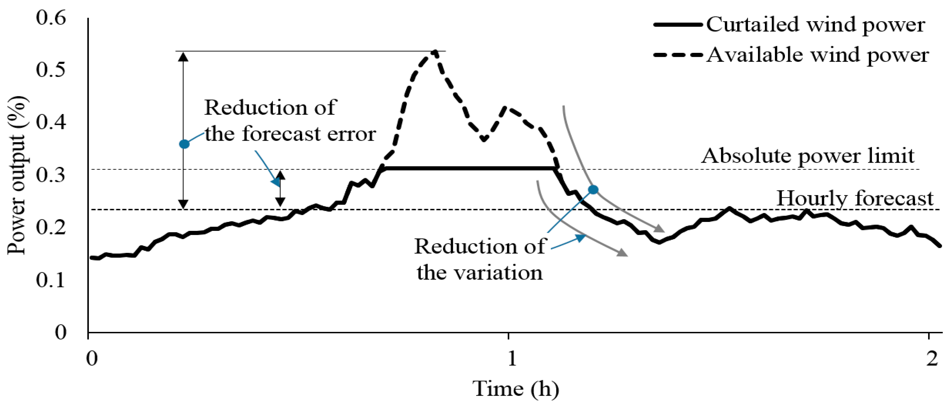
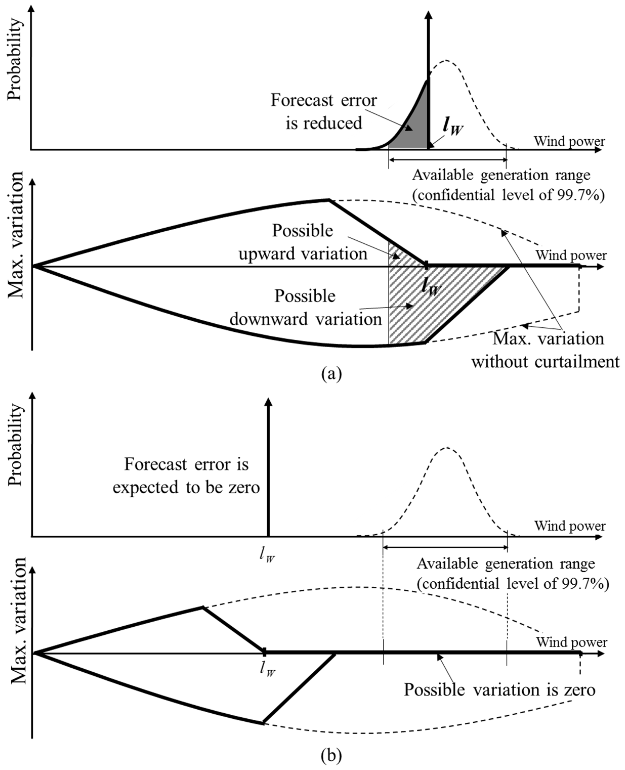
2.1. Mitigation of the Wind Power Forecast Uncertainty

The available wind power generation (pAW) of a wind farm is assumed to be subjected to a normal distribution, having a mean of the forecasted wind generation ( p A W f ) and a standard deviation derived from the forecast error (εW) as follows:
p A W = p A W f + ε W  
When wind power curtailment is executed with certain absolute power limit (lW) [15], then the wind power (pW) can be mathematically expressed as the following min function:
p W = min ( p A W f + ε W ,   l W )  
As wind generation is restricted to be below the absolute power limit and as the wind generation range is reduced, the uncertainties associated with the forecasting error will be reduced as shown in Figure 1. This advantage of uncertainty reduction leads to operational benefits that can reduce the required spinning reserve against the forecasting error.
As the wind energy in excess of the absolute power limit is spilled, the expected (forecasted) value of wind power production is decreased to less than that of the available wind power. The expected value of the delivered wind generation is derived from the definition of the expected value [16] for a non-negative random variable as follows:
p W f = 0 P W max ( 1 - F W ( p W ) ) d p W = 0 l W ( 1 - F A W ( p A W ) ) d p A W  
where FW and FAW represent the cumulative distribution functions (CDF) of the delivered wind generation and the available wind generation, respectively. Note that the CDF of the delivered wind generation between lW and P W max is equal to one, and the CDF of the delivered wind generation is equal to that of the available wind generation between lW and zero.

2.2. Mitigation of the Wind Power Variation

The simplest measure of wind power variation is a step change [17] in the average power between two consecutive times. For a time step τ, the maximum upward and downward variations are defined as follows:
u v A W = max ( p A W ,   t + τ p A W , t )  
d v A W = min ( p A W ,   t + τ p A W , t )  
where uvAW and dvAW are the maximum upward and downward variations of wind power, respectively; pAW,t and pAW,t+τ represent the wind power output at the initial time and after a time τ, respectively.
The wind power variation is subject to a different distribution depending on the given initial wind output [1]. The maximum variations in wind power that are obtained from the historical wind power data from Jeju in Korea are shown in Figure 2. With this dependency, the maximum upward and downward variations in wind power are defined as functions of the initial wind power.
With a given available wind power pAW, wind generation positively varies up to pAW + uvAW(pAW) when there is no limitation. However, when wind curtailment is executed, the wind power varies up to the lower value between the two absolute power limits of lW and pAW + uvAW(pAW). The maximum upward variation (uvW) of the wind generation can be therefore expressed as follows:
u v W ( p A W ) = min ( p A W + u v A W ( p A W ) ,   l W ) p W  
where uvAW(pAW) is the maximum upward variation without wind curtailment, which is a function of available wind power.
On the other hand, the downward variation in wind power is reduced because of the restriction of the initial wind power to be below the absolute power limit. With a given available wind power of pAW, wind generation negatively varies up to pAWdvAW(pAW) when there is no limitation. When wind power curtailment is executed, initial wind power is restricted to be the lower value between the absolute power limit lW and the available wind power pAW, and this wind generation can vary up to pAWdvAW(pAW). The maximum downward variation (dvW) in the wind generation can be therefore expressed as follows:
d v W ( p A W ) = p W   min ( p A W   d v A W ( p A W ) ,   l W )  
where dvAW(pAW) is the maximum downward variation without wind curtailment in terms of available wind power.
Figure 3 shows an example of maximum variation in wind power generation with different absolute power limits. With an absolute power limit within the available generation range as shown in Figure 3a, the maximum upward variation is considerably decreased, while it cannot be expected that the maximum downward variation will decrease. In case an absolute power limit is significantly lower than the available generation range as shown in Figure 3b, it is expected that the wind power forecast error will be approximately zero because almost all the possible wind generations will be restricted by the absolute power limit. It can be also expected that the wind power stays constant without any variation in both the directions.

2.3. Daily EV Charging Load

The EV charging load is modeled as a random variable while considering both the randomness of the activation time for charging the battery as well as the initial state of charge (SoC) at the beginning of the charging process. Once an EV starts charging at time tcs and continues to be charged until time t, the battery SoC will be increased from the initial SoC with the rated charging power until the battery reaches full capacity. The battery SoC (St) at time t can be expressed with the initial SoC (Sini) as follows:
S t =   S i n i + ( t t c s ) ( η E V P E V r ) / C E V  
where ηEV is the charging efficiency considering the efficiency of the battery itself and the charger; P E V r and CEV are the rated powers of the charger and the battery capacity, respectively. The initial SoC can be derived from daily travel distance [18].
Figure 4 shows a change in the probability density of the SoC by charging for one hour. After the EV charges for one hour, the SoC increases such that the SoC distribution is shifted toward a higher SoC region. As the charging duration increases, the probability of the EV being fully charged will increase.
Given that an EV starts charging at time tcs, the probability of an event (Ct) in which the EV is not fully charged until time t is calculated as follows:
pr ( C t |   t c s ) = pr ( S i n i + ( t t c s ) ( η E V P E V r ) / C E V   <   S max ) = F i n i ( S max ( t t c s ) ( η E V P E V r ) / C E V )   ,
where Fini is the CDF of the initial SoC. If an EV that starts charging at time tcs (before time t) does not reach a maximum SoC until time t, then the EV is still in charging mode at time t. Based on the total probability theorem [16], the probability that an EV is in charging mode at time t is expressed as follows:
pr ( C t )   = t c s = 1 N T { p r ( t c s ) F i n i ( S max ( t t c s ) ( η E V P E V r ) / C E V ) }  
where pr(tcs) is the probability that an EV starts charging at time tcs. From Bernoulli trials of Ct, the number of EVs that will be in the charging state is subject to a binomial distribution of B(NEV,pr(Ct)), which can be approximated as a normal distribution. Consequently, the total EV charging demand at time t is subject to a normal distribution with following mean and variance:
μ E V , t = P E V r N E V pr ( C t )  
  σ E V , t 2 = P E V r N   E V pr ( C t ) { 1 pr ( C t ) }  
The EV charging load can be merged with non-EV load by summation of the two normal distributions, and this load is used in the generation scheduling procedure as described in the following section.

3. Formulation of the Wind Power Curtailment Scheduling Problem

The generation scheduling problem with wind power curtailment is formulated in this section. The objective of this scheduling problem is to determine the generation and spinning reserves of conventional units and also the absolute power limit for wind generators that minimizes the operational cost as follows:
M i n   t = 1 N T i = 1 N G { C G , i ( p G , i , t ) + C S , i ( u i , t ) + C U R r u p ,   i , t + C D R r d n ,   i , t }  
where CG,i and CS,i are the generation cost and start-up cost of unit i respectively; pG,i,t and ui,t are the scheduled generation and on/off states of unit i at time t; rup.i,t and rdn.i,t represent the upward and downward spinning reserve deployed for unit i at time t, respectively; CUR, and CDR are the upward and downward reserve costs respectively; and NT and NG are the number of time intervals and the number of conventional units, respectively. The objective function (13) is subject to the following constraints.

3.1. Constraints for the Expected Wind Power and Load

3.1.1. Active Power Balance Equations

i = 1 N G p G , i , t + i = 1 N W 0 l W , i , t ( 1 - F A W ( p A W , i , t ) ) d p A W = i = 1 N B p D , i , t f ,      i , t ,
where the superscript f denotes the expected value of the random variables, and pD,i,t is the load on bus i at time t, which is the sum of the EV load and the non-EV load.
1.
Operating limits of the conventional units:
p G , i , t + r u p , i , t P i max u i , t ,      i , t ,
p G , i , t r d n , i , t P i min u i , t ,      i , t ,
where P i max and P i min are the maximum and minimum generation limits of generator i, respectively.
2.
Minimum up and down time limits:
( X i , t o n T i o n ) ( u i , t 1 u i , t ) 0 ,      i , t ,
( X i , t 1 o f f T i o f f ) ( u i , t u i , t 1 ) 0 ,      i , t ,
where X i , t o n and X i , t o f f are respectively the turn-on and turn-off periods before time t, and T i o n and T i o f f are the minimum up and down times of unit i.
3.
Hourly ramp up/down limits of the conventional unit:
p G , i , t p G , i , t 1 U R i max 60 ,       i , t ,
p G , i , t 1 p G , i , t D R i max 60 ,       i , t ,
where U R i max and D R i max are respectively the upward and downward maximum ramping rates of generator i.

3.1.2. Constraints for the Uncertain Wind and Load Scenario

1.
Active power balance for scenarios:
i = 1 N G p G , i , t s + i = 1 N W p W , i , t s   = i = 1 N B p D ,   i , t s ,      i , t , s ,
where p G ,   i , t s is the power generated by unit i at time t under scenario s, and p W ,   i , t s and p D ,   i , t s respectively represent the wind power generated and the load for scenarios.
2.
Absolute power limits of the wind farm for scenarios:
p W , i , t s = min ( p A W ,   i ,   t s ,   l i ,   t ) ,       i , t , s ,
where p A W ,   i ,   t s is the randomly sampled available wind generation for scenarios.
3.
Generation limits of the conventional unit for scenarios:
p G , i , t s + r e g u p , i , t s p G , i , t + r u p , i , t ,      i , t , s ,
p G , i , t s r e g d n , i , t s p G , i , t r d n , i , t ,      i , t , s ,
where r e g u p , i , t s and r e g d n , i , t s are respectively the upward and downward regulation powers required under scenarios. These constraints ensure that the generation and regulation powers of a unit are under its scheduled capacity limit.
4.
Ramping capability limits of the unit for scenarios:
r e g u p , i , t s U R i max τ u i , t ,       i , t , s ,
r e g d n , i , t s D R i max τ u i , t ,       i , t , s ,
These constraints ensure that a generation unit can increase or decrease its regulation power by changing its ramping rates appropriately during a certain time period τ.
5.
System ramping requirements for scenarios:
i = 1 N G r e g u p , i , t s i = 1 N W d v W ( p A W , i , t s ) + u v D ,       i , t , s ,
i = 1 N G r e g d n , i , t s i = 1 N W u v W ( p A W , i , t s ) + d v D ,       i , t , s ,
where uvD and dvD represent the maximum short-term variations of the system load, which are assumed to be identical over the time period; uvAW( p A W , i , t s ) and dvAW( p A W , i , t s ) are the maximum upward and downward variations for scenario s, which were derived in (6) and (7).
The above formulation is a large-scale, mixed-integer nonlinear problem (MINLP), because it contains the continuous integral for the expected wind power in (14) and the min-function for the absolute power limit in (19). In order to avoid this computational intractability, a nonlinear structure in the above model is transformed into MIP forms by discretizing random variables, which is described in the following section.

4. Scenario Based Wind Curtailment Scheduling

4.1. Random Variable Discretization for Absolute Power Limit

For a scenario-based stochastic UC model, the continuous probability distribution model of wind generation is not computationally practical. Instead, it is more reasonable to consider discretization of the continuous probability distribution of the wind generation with a number of representative segments. This paper uses a discretized random variable [11] of wind generation with Nm segments, which equally divides the available wind generation region. The discrete random variable of wind generation si,t(m) is defined as a value at the center of the mth segment, and its probability is calculated by integrating the continuous probability within the corresponding segment.
With this discrete random variable of wind generation, the absolute power limit can be expressed as follows:
l W , i , t = m = 1 N m ( s i , t ( m ) s i , t ( m 1 ) ) u L , i , t ( m ) ,
where si,t(m) is the discrete random variable of wind generation of wind farm i at time t; uL,i,t(m) is the binary variable that indicates whether the absolute power limit is greater than si,t(m) or not, and uL,i,t(m) is restricted to be lower than or equal to uL,i,t(m − 1). In the same way, p A W , i , t s , p A W , i , t s + uvAW( p A W , i , t s ), and p A W , i , t s dvAW( p A W , i , t s ) can be also expressed in terms of the discrete random variable of wind generation and also the binary variables u A W , i , t s (m), u u v , i , t s (m), and u d v , i , t s (m), respectively.
With the discrete random variable of wind generation, the expected wind power with wind curtailment in (3) can be rewritten as follows:
p W , i , t f = m = 1 N m { ( s i , t ( m ) s i , t ( m 1 ) ) u L , i , t ( m ) n m N m pr ( s i , t ( n ) ) } .
Absolute power constraints for scenarios in (19) can be expressed as follows:
p W , i , t s = m = 1 N m { ( s i , t ( m ) s i , t ( m 1 ) ) u A W , i , t s ( m )   u L , i , t ( m ) } .
Note that the minimum of two binary variables is equal to their product. In the same way, the maximum upward and downward variation in wind generation for scenario s of (6) and (7) can be rewritten in the following MIP forms:
u v W ( p A W , i , t s ) = m = 1 N m { ( s i , t ( m ) s i , t ( m 1 ) ) u u v , i , t s ( m ) u L , i , t ( m ) } p W , i , t s ,
d v W ( p A W , i , t s ) = p W , i , t s m = 1 N m { ( s i , t ( m ) s i , t ( m 1 ) ) u d v , i , t s ( m ) u L , i , t ( m ) }  
All constraints of the wind curtailment scheduling problem can be transformed into MIP forms with the help of discrete random variable of wind generation.

4.2. Decomposition of the Stochastic UC Problem

The paper decomposes the original UC problem in Section 4 into a deterministic UC problem and a flexibility-checking sub-problem using Benders decomposition. The deterministic UC problem solves the optimization problem using the objective function in (13) subject to the constraints in (14)–(17). In the deterministic UC problem, forecasted wind power is substituted by (24).
Under a specific scenario for uncertain wind and load, the deterministic UC solution may fail to adjust the generation level due to insufficient spinning reserve and ramping capability. In such cases, the system flexibility needs to be increased by deploying an additional spinning reserve or by scheduling wind power curtailment by following a flexibility-checking sub-problem for all scenarios shown below:
R t s = M i n i m i z e   e u s r , t s + e d s r , t s + e u r e g , t s + e d r e g , t s   ,
Subject to:
i = 1 N G p G , i , t s + i = 1 N W p W , i , t s   = i = 1 N B p D ,   i , t s e u s r , t s + e d s r , t s   ,
p W , i , t s = m = 1 N m { ( s i , t ( m ) s i , t ( m 1 ) ) u A W , i , t s ( m )   u ^ L , i , t ( m ) }   ,
e u r e g , t s + i = 1 N G r e g u p , i , t s u v D + i = 1 N W p W , i , t s   i = 1 N W m = 1 N m { ( s i , t ( m ) s i , t ( m 1 ) ) u d v , i , t s ( m ) u ^ L , i , t ( m ) }  
e d r e g , t s + i = 1 N G r e g d n , i , t s d v D i = 1 N W p W , i , t s + i = 1 N W m = 1 N m { ( s i , t ( m ) s i , t ( m 1 ) ) u u v , i , t s ( m ) u ^ L , i , t ( m ) }  
and also subject to the constraints (20) and (21), where the variables with caret on their top are the solutions of the deterministic UC. If an objective value is greater than zero, then the solution of the deterministic UC problem cannot ensure operational security against both the forecast error and the short-term variations for a specific scenario. In this case, the following reliability cuts will be generated and added to the deterministic problem for the next iteration:
e ^ u s r , t s + e ^ u r e g , t s + i = 1 N W m = 1 N m m t s ( u ^ L , i , t ( m ) ) ( u L , i , t ( m ) u ^ L , i , t ( m ) ) + i = 1 N G m t s ( p ^ G , i , t ) ( p G , i , t p ^ G , i , t )   + i = 1 N G   m t s ( r ^ u p ,   i , t ) ( r u p , i , t r ^ u p ,   i , t ) 0  
e ^ d s r , t s + e ^ d r e g , t s + i = 1 N W m = 1 N m m t s ( u ^ L , i , t ( m ) ) ( u L , i , t ( m ) u ^ L , i , t ( m ) )   + i = 1 N G m t s ( p ^ G , i , t ) ( p G , i , t p ^ G , i , t )   + i = 1 N G   m t s ( r ^ d n ,   i , t ) ( r d n , i , t r ^ d n ,   i , t ) 0  
where m t s (·) is a marginal value of the objective function (28a) with respect to a corresponding variable at the solutions of the deterministic UC problem.
After checking the flexibility of the power system for all scenarios, the original probability density function (pdf) of wind and load will be updated using the following formula of cross-entropy method [19]:
μ n = s = 1 N S I ( R t s γ ^ n ) W s P t s / s = 1 N S I ( R t s γ ^ n ) W s ,
σ n   = s = 1 N S I ( R t s γ ^ n ) W s ( P t s μ n ) 2 / s = 1 N S I ( R t s γ ^ n ) W s ,
where the function I( m t s ≥ 0) is equal to one if m t s ≥ 0, is equal to zero otherwise. Ws is a likelihood ratio vector between the probability rate of the initial pdf and the updated pdf at the sampled value P t s . This pdf update causes violation events to occur more frequently so that a more critical event can be rapidly checked in the sub-problems.

5. Numerical Results

5.1. Test System

The proposed method was tested using the IEEE Reliability Test System [20]. In the base case, three wind farms are included in place of hydro generators of the original RTS-96. The total installed capacity of the three wind farms is 450 MW, which is 12% of the installed generation capacity. The yearly peak load is set to be 2850 MW, and a load profile of first week of [20] was used. The fuel price is obtained from [21], but the fuel price of number 2 oil was set to be the same as that of number 6 oil. Upward and downward reserve costs of every generators are assumed to be 10 $/MW and 5 $/MW, respectively. The day-ahead load forecast error was assumed to be a zero-mean normal distribution with a standard deviation of 2% of the forecasted load. The maximum short-term load variations were calculated from the historical data of Korea during 2010, and were set as 1.2% of the hourly load for both directions. The time step (τ) was set to be five minutes, which is equal to the dispatch interval of automatic generation control.
Furthermore, the hourly wind power forecast was obtained by utilizing a moving average model with hourly measurements of five wind farms in Korea in 2010. The available wind generation range was set between three times of the standard deviations. The maximum wind power variations were also calculated using the historical data of Korea as shown in Figure 2.
The total number of private vehicles was assumed to be seven hundred thousand, which is scaled down from that of the private vehicles in Korea considering the total capacity of the test system. In the base case, the number of EVs was assumed to be 20% of private vehicles. The battery capacity of an EV was assumed to be 16 kWh. It was assumed that the EVs are charged only at home with 1.44 kW rated power. The daily travel distance is assumed to be log-normally distributed with a mean of 36.9 km and with a standard deviation of 23.4 km obtained from [22]. The start time of charging is obtained from the distribution of departure time [22] with an assumption that the EVs begin charging one hour after their departure from work.

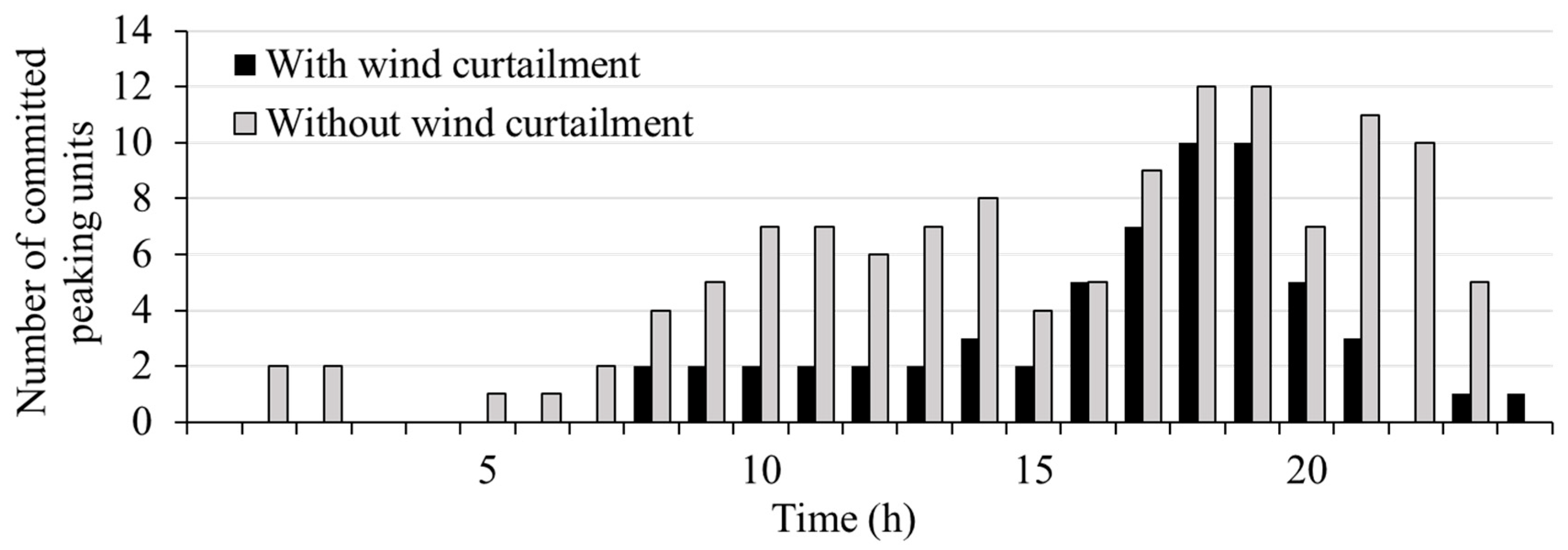
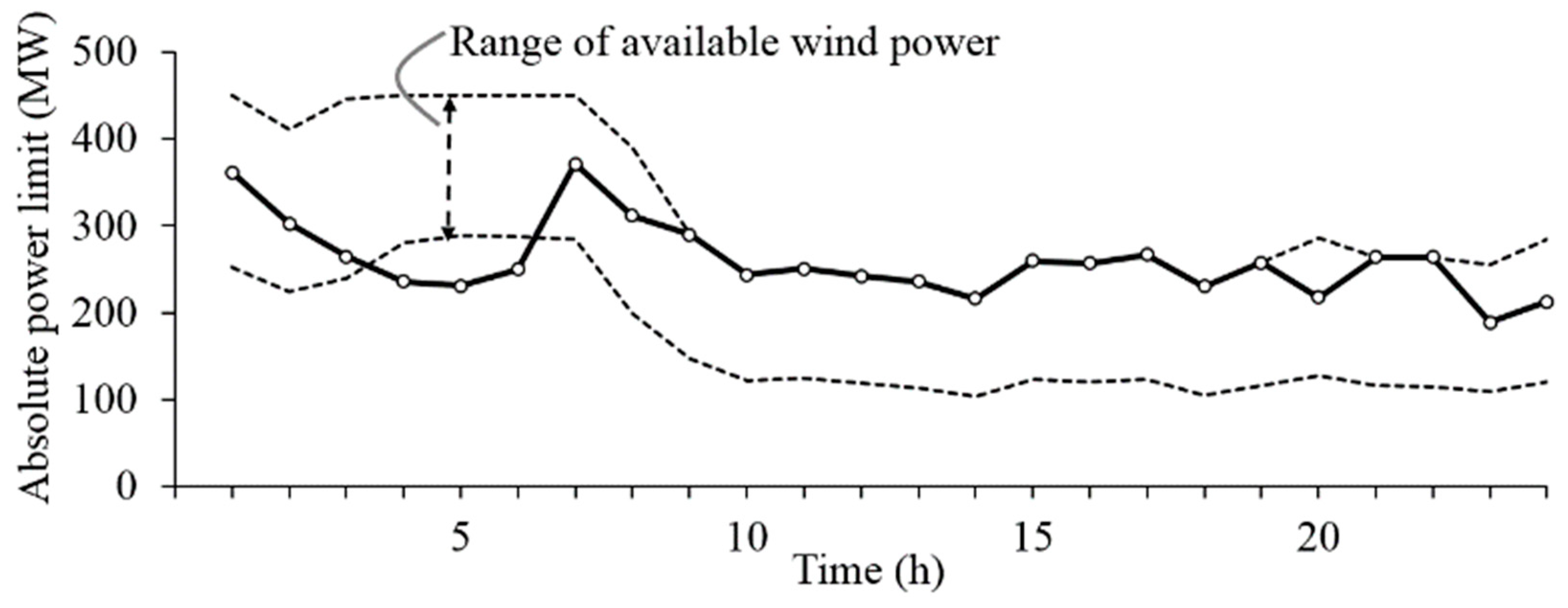
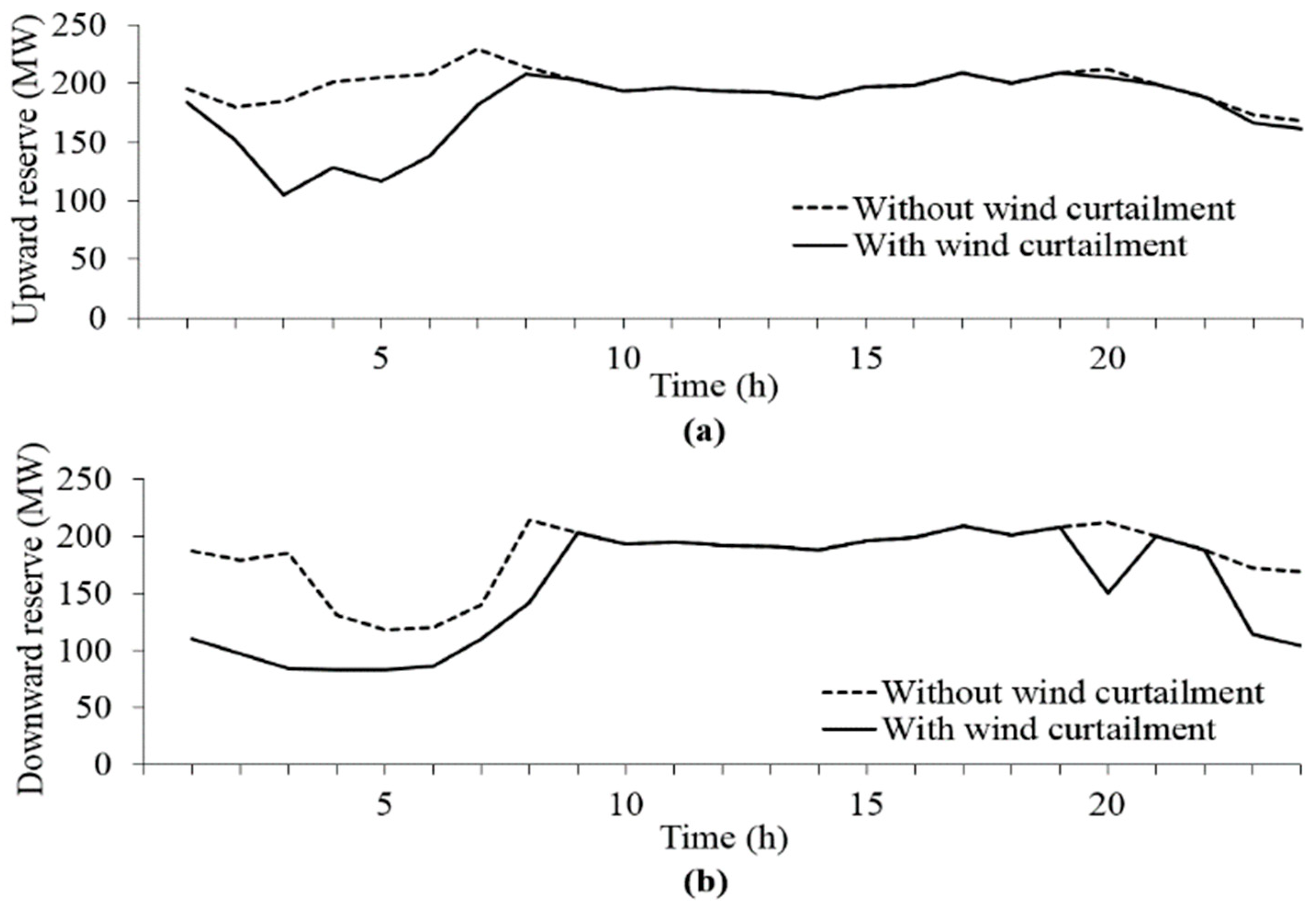
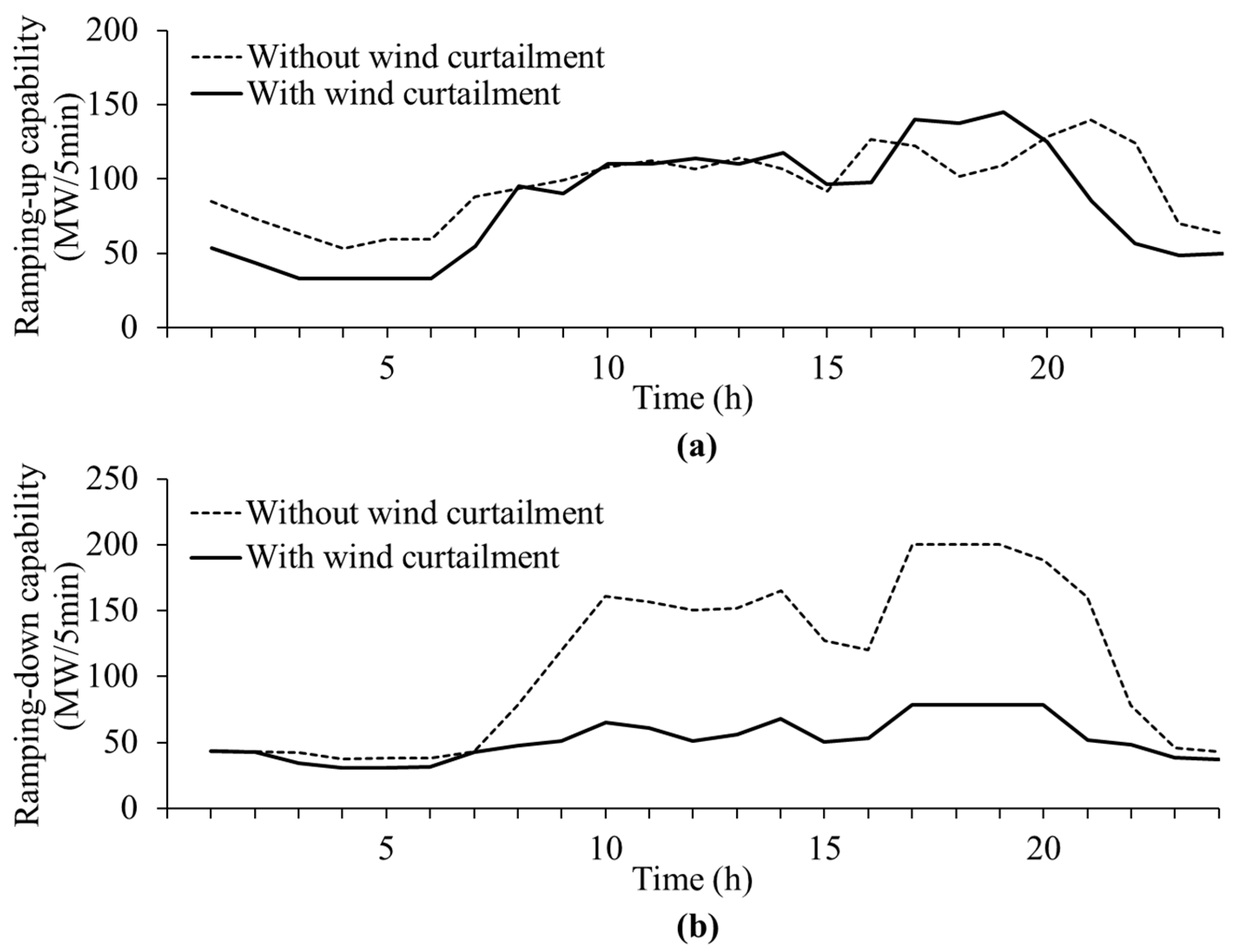
5.2. Results of Wind Power Curtailment Scheduling

In the solution without wind curtailment, one of the two nuclear units needs to be turned off in order to ensure sufficient downward reserve capacity. While in the case with wind curtailment, as wind generation is reduced, generation levels of the other units can be increased enough so that sufficient downward reserve capacity is ensured. Therefore, both nuclear generators do not have to be turned off.
Figure 5 shows the number of committed peaking units with and without wind curtailment. In the UC problem with wind curtailment, a fewer number of peaking units need to be turned on for all the time periods. This is because wind curtailment contributes to the mitigation of short-term variations of wind power at night. By incorporating wind curtailment, it is able to compensate for short-term wind variations without any fast responding peaking generator.
Figure 6 shows the scheduled absolute power limits of the UC schedule with wind curtailment. A portion of wind curtailment is to avoid oversupply of wind generation, which enforces baseload generators to be turned off. Wind curtailment during 4–6 h is attributed to an oversupply of wind generation because an absolute power limit that is set to be the lowest available wind power is sufficient to fully mitigate the wind power uncertainties. The remaining portion of the wind curtailment is attributed to expensive spinning reserves to be scheduled against wind power uncertainty. At 20 h and during 23–24 h, wind generation is curtailed for this reason because there is no need to be concerned about an oversupply during these times.
Figure 7 shows the results of the scheduled spinning reserve with and without the implementation of wind curtailment. During 1–8 h, 21 h, and 23–24 h, a lower spinning reserve is scheduled with wind curtailment implemented than that without the implementation of wind curtailment. It can be concluded that the wind curtailment makes it possible to ensure operational security with a lower reserve capacity.
Figure 8 shows the system ramping capabilities in both cases with and without wind curtailment. By scheduling the wind curtailment, the proposed method provides a UC solution that is capable of compensating for short-term wind variations with lower ramping capability. Because of mitigation of short-term variations, the fast responding peaking units need not replace the baseload units for improving the ramping capability of the system, and this leads to a decrease in the operation cost.
Table 1 summarizes a comparison of the simulation results of generation scheduling in cases that do and do not implement wind power curtailment. The energy cost is generally expected to increase with wind curtailment because significant zero cost wind energy will be wasted. However, the results in Table 1 are in contrast to this expectation. In order to avoid oversupply without wind curtailment, baseload generators may need to be turned off, and other expensive generators need to replace them because of their minimum generation level. Once the baseload generators are turned off, they cannot be brought into operation again soon because of the minimum down time constraint. Consequently, without wind curtailment, more expensive generators need to be scheduled, and this leads to an increase in the operational cost.

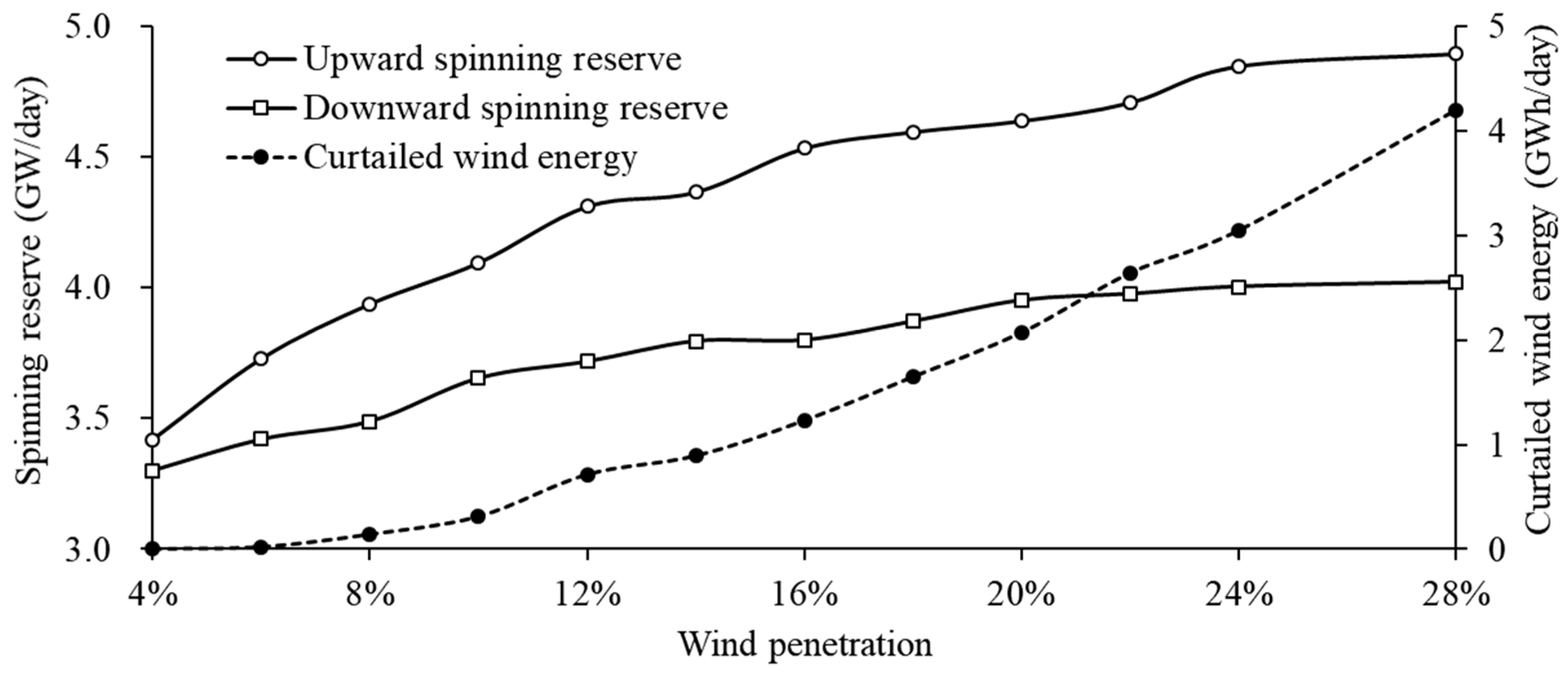
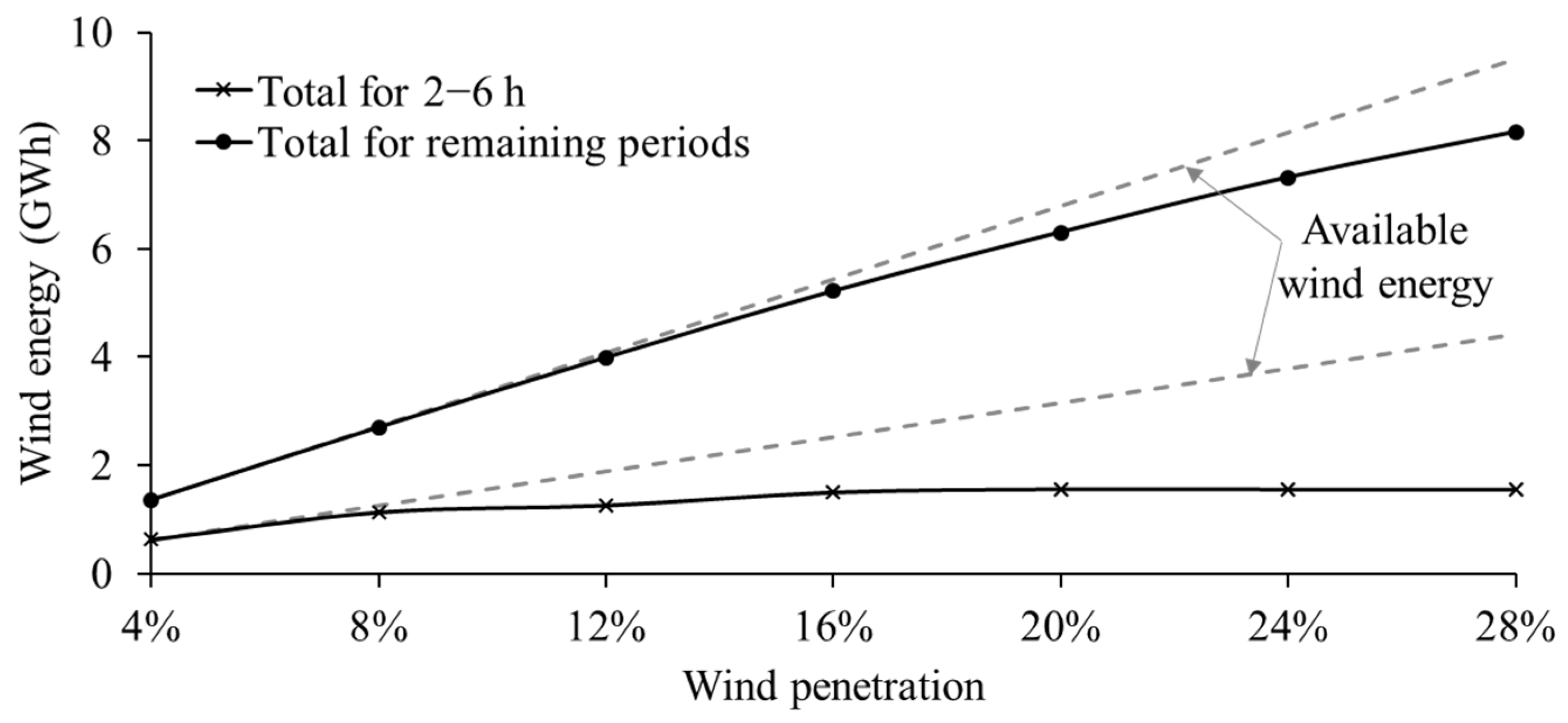
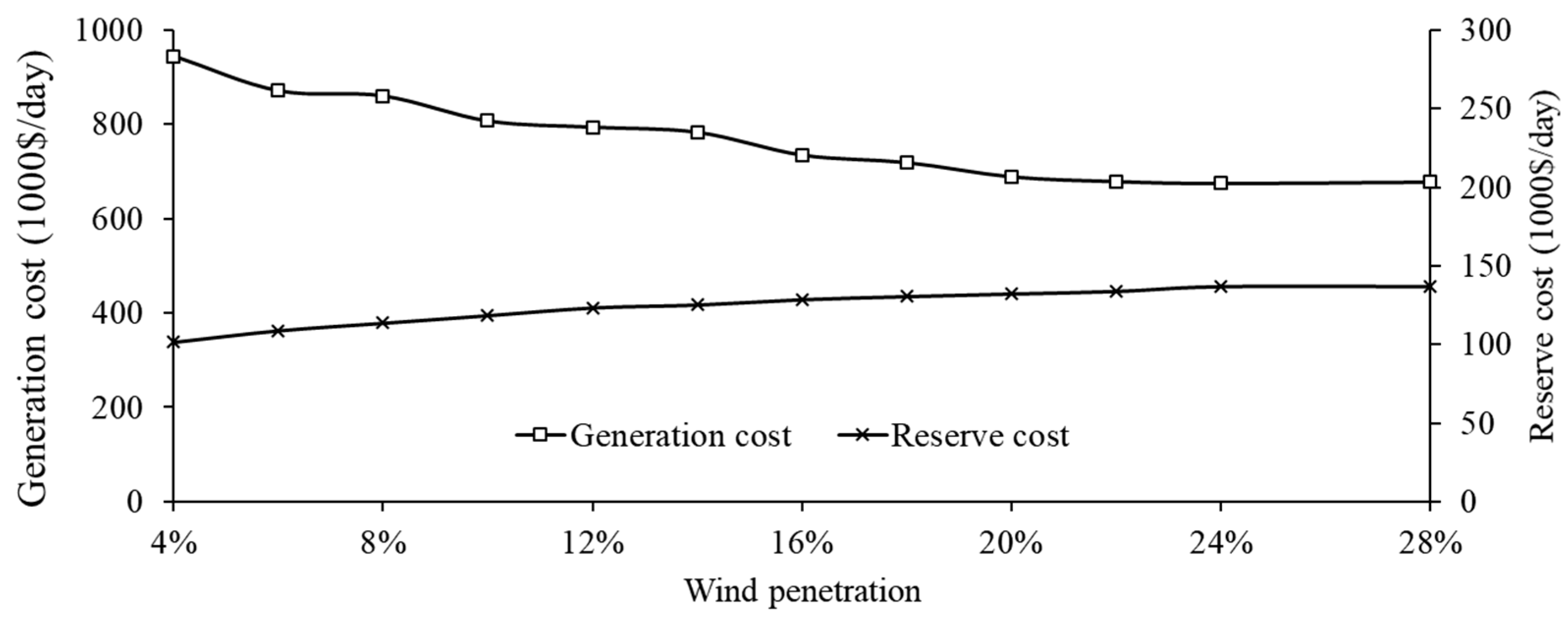
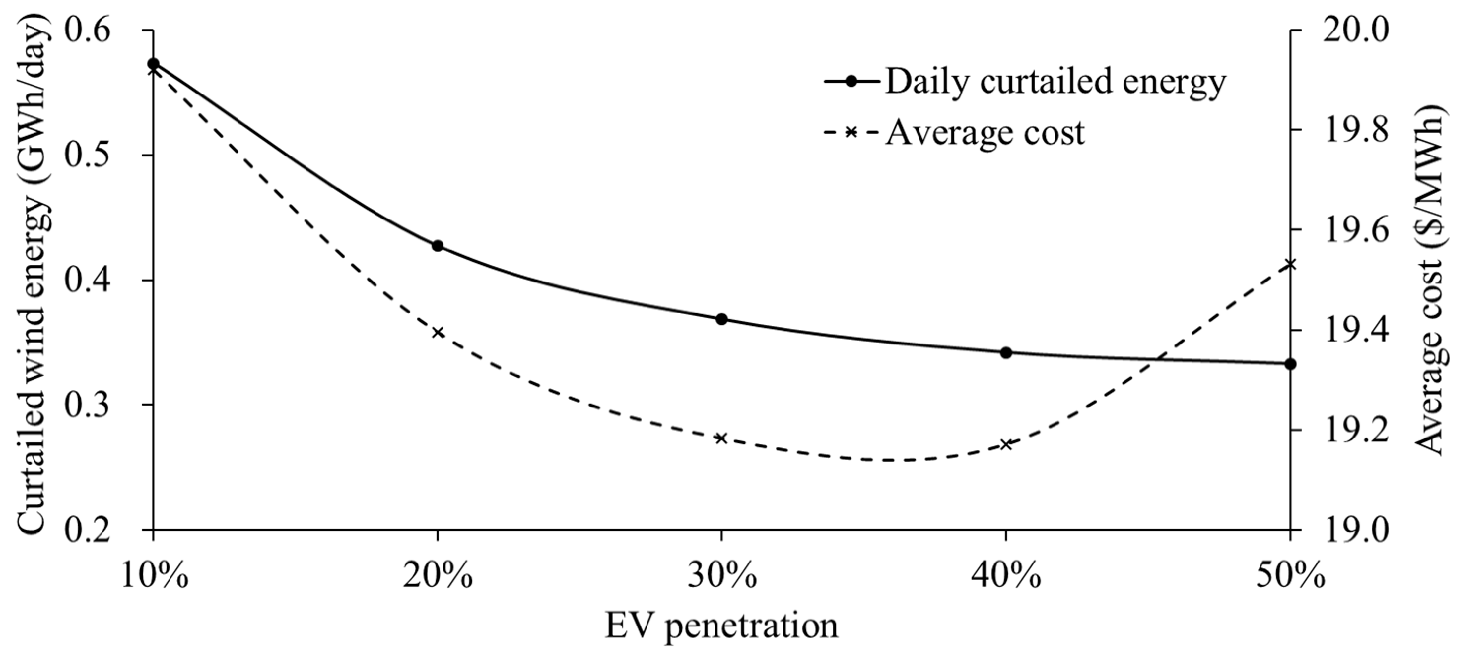
5.3. Influence of Wind and EV Penetration

This section shows the simulation results with different wind power and EV penetration levels. It is assumed that the forecasting error and short-term variations linearly increase according to the wind farm capacity.
Figure 9 shows the scheduled spinning reserve and curtailed wind energy with different wind penetration levels. At lower wind penetration levels, wind farms are allowed to generate their available wind generation without any curtailment. At higher wind penetration levels, a good amount of wind energy is scheduled to be curtailed because of the increased forecasting error and short-term variations as well as the increased oversupply. Both spinning reserves are significantly increased as the wind penetration increases. However, at higher wind penetration levels, there is a decrease in the increasing rates of spinning reserves because more wind curtailment is scheduled to relieve the oversupply and wind power uncertainty is mitigated.
Figure 10 shows the scheduled wind energy with different wind penetration levels. During 2–6 h, wind farms are not allowed to generate their available wind energy beyond 1500 MWh through wind capacity increases because of an oversupply of wind generation. During the remaining periods (1 h and 7–24 h), it is observed that curtailed wind energy is exponentially increased as the wind penetration increases. This is attributed to the reason that the incremental cost of one MW spinning reserve is increased as the required spinning reserve increases.
Figure 11 shows the operational costs incurred with different wind power penetration levels. It can be figured out that unit wind energy value is decreased as a greater number of wind generators are installed, and wind energy beyond a certain penetration level cannot give economic benefits to the power system.
Figure 12 shows the daily curtailed wind energy and average operation costs for different EV penetration levels. As the EV penetration level increases, the EV charging load is expected to have less effect on the wind power curtailment. The average cost decreases as the EV penetration increases up to 30%, because more wind energy can be used as a result of relieving the oversupply by the additional demand of EVs. Beyond 30%, the oversupply is sufficiently relieved, and EVs act as additional demands, thereby leading to an increase in the average cost.

6. Conclusions

This paper presents a stochastic generation scheduling method incorporating wind power curtailment, which reduces the reserve and ramping capability requirements. The wind power curtailment could contribute not only to relieving the oversupply, but also to mitigate the short-term variations of wind power. In the test results, EVs are also seen to relieve the oversupply of wind power so that more wind energy can be used, and the average cost is decreased up to a certain level of EV penetration. The proposed method can also be used for scheduling the operation of the power systems, which suffer from light load conditions due to high wind capacity.

Author Contributions

J.L. (Jaehee Lee) developed the idea and scheduling models, performed model simulations, analyzed the data, and wrote the paper. J.L. (Jinyeong Lee) and Y.-M.W. helped organize the article. S.-K.J. provided guidance for the research and revised the paper.

Acknowledgments

This work was supported by the National Research Foundation of Korea (NRF) grant funded by the Korea government (MSIT) (No. 2017R1C1B5016244). This research was supported by the Korea Electric Power Corporation (Grant number: R18XA04).

Conflicts of Interest

The authors declare no conflict of interest.

References

  1. Dragoon, K. Chapter 5-Representing Wind in Economic Dispatch Models. In Valuing Wind Generation on Integrated Power Systems, 1st ed.; Elsevier: Oxford, UK, 2010. [Google Scholar]
  2. Fink, S.; Mudd, C.; Porter, K.; Morgenstern, B. Wind Energy Curtailment Case Studies: May 2008−May 2009; National Renewable Energy Laboratory: Golden, CO, USA, 2009.
  3. Gu, Y.; Xie, L. Fast Sensitivity Analysis Approach to Assessing Congestion Induced Wind Curtailment. IEEE Trans. Power Syst. 2014, 29, 101–110. [Google Scholar] [CrossRef]
  4. Daneshi, H.; Srivastava, A.K. Security-Constrained Unit Commitment with Wind Generation and Compressed Air Energy Storage. IET Gener. Transm. Distrib. 2012, 6, 167–175. [Google Scholar] [CrossRef]
  5. Gu, Y.; Xie, L. Look-ahead Coordination of Wind Energy and Electric Vehicles: A Market-Based Approach. In Proceedings of the North American Power Symposium 2010, Arlington, TX, USA, 26–28 September 2010. [Google Scholar]
  6. Dui, X.; Zhu, G.; Yao, L. Two-Stage Optimization of Battery Energy Storage Capacity to Decrease Wind Power Curtailment in Grid-Connected Wind Farms. IEEE Trans. Power Syst. 2018, 33, 3296–3305. [Google Scholar] [CrossRef]
  7. Restrepo, J.; Galiana, F. Assessing the Yearly Impact of Wind Power Through a New Hybrid Deterministic/Stochastic Unit Commitment. IEEE Trans. Power Syst. 2011, 26, 401–410. [Google Scholar] [CrossRef]
  8. Wang, C.; Lu, Z.; Qiao, Y. A Consideration of the Wind Power Benefits in Day-Ahead Scheduling of Wind-Coal Intensive Power Systems. IEEE Trans. Power Syst. 2013, 28, 236–245. [Google Scholar] [CrossRef]
  9. Wang, C.; Liu, T.; Zhu, Z.; Cheng, J.; Wei, C.; Wu, Y.; Lin, C.; Bai, F. A Probabilistic Day-ahead Scheduling with Considering Wind Power Curtailment. In Proceedings of the IEEE Conference on Energy Internet and Energy System Integration, Beijing, China, 26–28 November 2017. [Google Scholar]
  10. Li, C.; Ahn, C.; Peng, H.; Sun, J. Synergistic Control of Plug-In Vehicle Charging and Wind Power Scheduling. IEEE Trans. Power Syst. 2013, 28, 1113–1121. [Google Scholar] [CrossRef]
  11. Bouffard, F.; Galiana, F.D. Stochastic Security for Operations Planning with Significant Wind Power Generation. IEEE Trans. Power Syst. 2008, 23, 306–316. [Google Scholar] [CrossRef]
  12. Wang, J.; Shahidehpour, M.; Li, Z. Security-Constrained Unit Commitment with Volatile Wind Power Generation. IEEE Trans. Power Syst. 2008, 23, 1319–1327. [Google Scholar] [CrossRef]
  13. Fu, Y.; Shahidehpour, M.; Li, Z. Security-Constrained Unit Commitment with AC Constraints. IEEE Trans. Power Syst. 2005, 20, 1538–1550. [Google Scholar] [CrossRef]
  14. Hillier, F.S.; Lieberman, G.J. Introduction to Operation Research, 9th ed.; McGraw-Hill: New York, NY, USA, 2010; pp. 464–536. ISBN 13: 978-0077298340. [Google Scholar]
  15. Tsili, M.; Papathanassiou, S. A Review of Grid Code Technical Requirements for Wind Farms. IET Renew. Power Gen. 2009, 3, 308–332. [Google Scholar] [CrossRef]
  16. Leon-Garcia, A. Probability and Random Processes for Electrical Engineering, 2nd ed.; Addison-Wesley: Boston, MA, USA, 1994; pp. 126–288. ISBN 13: 978-0201500370. [Google Scholar]
  17. Wan, Y.; Bucaneg, D. Short-Term Power Fluctuations of Large Wind Power Plants. J. Sol. Energy Eng. 2002, 124, 427–431. [Google Scholar] [CrossRef]
  18. Qian, K.; Zhou, C.; Allan, M.; Yuan, Y. Modeling of Load Demand Due to EV Battery Charging in Distribution Systems. IEEE Trans. Power Syst. 2011, 26, 802–810. [Google Scholar] [CrossRef]
  19. Rubinstien, R.Y.; Kroese, D.P. The Cross-Entropy Method, 1st ed.; Springer: New York NY, USA, 2004; pp. 59–128. ISBN 13: 978-0387212401. [Google Scholar]
  20. Grigg, C.; Wong, P.; Albrecht, P.; Allan, R.; Bhavaraju, M.; Billinton, R.; Chen, Q.; Fong, C.; Haddad, S.; Kuruganty, S.; et al. The IEEE Reliability Test System-1996. A report prepared by the Reliability Test System Task Force of the Application of Probability Methods Subcommittee. IEEE Trans. Power Syst. 1999, 14, 1010–1020. [Google Scholar] [CrossRef]
  21. Hedman, K.; Ferris, M.; O’Neill, R.; Fisher, E.; Oren, S. Co-Optimization of Generation Unit Commitment and Transmission Switching with N-1 Reliability. IEEE Trans. Power Syst. 2010, 25, 1052–1063. [Google Scholar] [CrossRef]
  22. 2011 Estimation of Vehicle Kilometers; Korea Transportation Safety Authority: Ansan, South Korea, December 2012; Available online: http://kiss.kstudy.com/public/public3-article.asp?key=60000130 (accessed on 19 August 2018).
Figure 1. Wind power curtailment using the absolute power limit.
Applsci 08 01684 g001
Figure 2. Maximum short-term variations in wind power with varying initial wind power levels: (a) upward variation and (b) downward variation.
Applsci 08 01684 g002
Figure 3. Maximum variation in wind power with different absolute power limits (lW): (a) absolute power limit within the available wind generation range and (b) absolute power limit that is significantly lower than the available generation.
Applsci 08 01684 g003
Figure 4. Change in the probability density of the state of charge (SoC) of an electric vehicle (EV) by charging for one hour.
Applsci 08 01684 g004
Figure 5. Number of committed peaking generators.
Applsci 08 01684 g005
Figure 6. Scheduled absolute power limit.
Applsci 08 01684 g006
Figure 7. Scheduled spinning reserve with and without wind curtailment: (a) upward spinning reserve and (b) downward spinning reserve.
Applsci 08 01684 g007
Figure 8. System-wide ramping capability with and without wind power curtailment: (a) ramping-up capability and (b) ramping-down capability.
Applsci 08 01684 g008
Figure 9. Scheduled spinning reserve and curtailed wind energy with different wind penetrations.
Applsci 08 01684 g009
Figure 10. Scheduled wind energy with different wind penetrations.
Applsci 08 01684 g010
Figure 11. Operational cost with different wind power penetrations.
Applsci 08 01684 g011
Figure 12. Curtailed wind energy and average cost with different EV penetrations.
Applsci 08 01684 g012
Table 1. Operational costs of unit commitment (UC) with and without wind curtailment.
Case without Wind CurtailmentCase with Wind Curtailment
Generation Cost1,331,004 $/day812,309 $/day
Reserve Cost138,529 $/day123,387 $/day
Total Cost 1,469,533 $/day935,696 $/day

