Research on a Surface Defect Detection Algorithm Based on MobileNet-SSD

Abstract

This paper aims to achieve real-time and accurate detection of surface defects by using a deep learning method. For this purpose, the Single Shot MultiBox Detector (SSD) network was adopted as the meta structure and combined with the base convolution neural network (CNN) MobileNet into the MobileNet-SSD. Then, a detection method for surface defects was proposed based on the MobileNet-SSD. Specifically, the structure of the SSD was optimized without sacrificing its accuracy, and the network structure and parameters were adjusted to streamline the detection model. The proposed method was applied to the detection of typical defects like breaches, dents, burrs and abrasions on the sealing surface of a container in the filling line. The results show that our method can automatically detect surface defects more accurately and rapidly than lightweight network methods and traditional machine learning methods. The research results shed new light on defect detection in actual industrial scenarios.

1. Introduction

Intellisense and pattern recognition technologies have made progress in robotics [1,2,3], computer engineering [4,5], health-related issues [6], natural sciences [7] and industrial academic areas [8,9]. Among them, computer vision technology develops particularly quickly. It mainly uses a binary camera, digital camera, depth camera and charge-coupled device (CCD) camera to collect target images, extract features and establish corresponding mathematical models, and to complete the processing of target recognition, tracking and measurement. For example, Kamal et al. comprehensively consider the continuity and constraints of human motion. After contour extraction of the acquired depth image data, the Hidden Markov Model (HMM) is used to identify human activity. This system is highly accurate in recognition and has the ability to effectively deal with rotation and deficiency of the body [10]. Jalal et al. use Texture and shape vectors to reduce feature vectors and extracts important features in facial recognition through density matching score and boundary fixation, so as to manage key processing steps of face activity (recognition accuracy, recognition speed and security) [11]. In [12], vehicle damage is classified by a deep learning method, and the recognition accuracy of a small data set was up to 89.5% by the introduction of transfer learning and an integrated learning method. This provides a new way for automatic processing of vehicle insurance. Zhang et al. combine the four features of color, time motion, gradient norm and residual motion to identify the position of each frame in video. The method uses weighted linear combination to evaluate the different combinations of these features and establishes a precise hand detector [13]. With the continuous improvement of computer hardware and the deepening of research on complex image classification, the application prospect of computer vision technology will be more and more extensive.

Surface defect detection is an important issue in modern industry. Traditionally, surface defects are often detected in the following steps: first, pre-processing of the target image by image processing algorithms. Image pre-processing technology can process pixels accurately. By setting and adjusting various parameters according to actual requirements, the image quality can be improved by de-noising, changing brightness and improving contrast, laying a foundation for subsequent processing; second, carry out histogram analysis, wavelet transform or Fourier transform. The above transformation methods can obtain the representation of an image in a specific space, which is convenient for the artificial designing and extracting feature; finally, the image is classified according to its features using a classifier. Common methods include thresholding, decision trees or support vector machine (SVM). Most of the existing surface defect detection algorithms are based on machine vision [14,15,16,17,18,19]. Considering the mirror feature of ceramic balls, [17] obtains the stripe distortion image of defective parts according to the principle of the fringe reflection and locates the defect positions by reverse ray tracing. The research method is suitable for surface defect detection of ceramic balls and other phases, but fails to achieve high accuracy due to the selection and design of radiographic models in reverse ray tracing. Jian et al. realize the automatic detection of glass surface defects on cell phone screens through fuzzy C-means clustering. Specifically, the image was aligned by contour registration during pre-processing, and then the defective area was segmented by projection segmentation. Despite the high accuracy, the detection approach consumes way too much time (1.6601 s) [18]. Win et al. integrate a median-based Otsu image thresholding algorithm with contrast adjustment to achieve automatic detection of the surface defects on titanium coating. The proposed method is simple and, to some extent, immune to variation in light and contrast. However, when the sample size is large, the optimal threshold calculation is too inefficient and the grey information is easily contaminated by dry noise points [19]. To sum up, the above surface detection methods can only extract a single feature, and derive a comprehensive description of surface defects from it. These types of approaches only work well on small sample datasets, but not on large samples and complex objects and backgrounds in actual production. To solve this problem, one viable option is to improve the approach with deep learning.

In recent years, deep learning has been successfully applied to image classification, speech recognition and natural language processing [20,21,22]. Compared with the traditional machine learning method, it has the following characteristics: deep learning can simplify or even omit the pre-processing of data, and directly use the original data for model training; deep learning is composed of multi-layer neural networks, which solve the defects in the traditional machine learning methods of artificial feature extraction and optimization. So far, deep learning has been extensively adopted for surface defect detection. For example, in [23], Deep Belief Network (DBN) was adopted to obtain the mapping relationship between training images of solar cells and non-defect templates, and the comparison between reconstructed images and defect images was used to complete the defect detection of the test images. Cha et al. employ a deep convolution neural network (CNN) to identify concrete cracks in complex situations, e.g. strong spots, shadows and ultra-thin cracks, and proves that the deep CNN outperformed the traditional tools like Canny edge detector and Sobel edge detector [24]. Han et al. detect various types of defects on hub surfaces with residual network (ResNet)-101 as the base net and the faster region-based CNN (Faster R-CNN) as the detector and achieves a high mean average precision of 86.3% [25]. The above studies fully verify the excellent performance of deep learning in detecting surface defects. Nevertheless, there are few studies on product surface defect detection using several main target detection networks in recent years, such as YOLO (You Only Look Once), SSD (Single Shot MultiBox Detector) [26] and so on. The detection performance of these networks in surface defect detection needs to be further verified and optimized.

This paper presents a surface defect detection method based on MobileNet-SSD. By optimizing the network structure and parameters, this method can meet the requirements of real-time and accuracy in actual production. It was verified in the filling line and the results show that our method can automatically locate and classify the defects on the surface of the products.

2. Surface Defect Detection Method

2.1. Image Pre-Processing

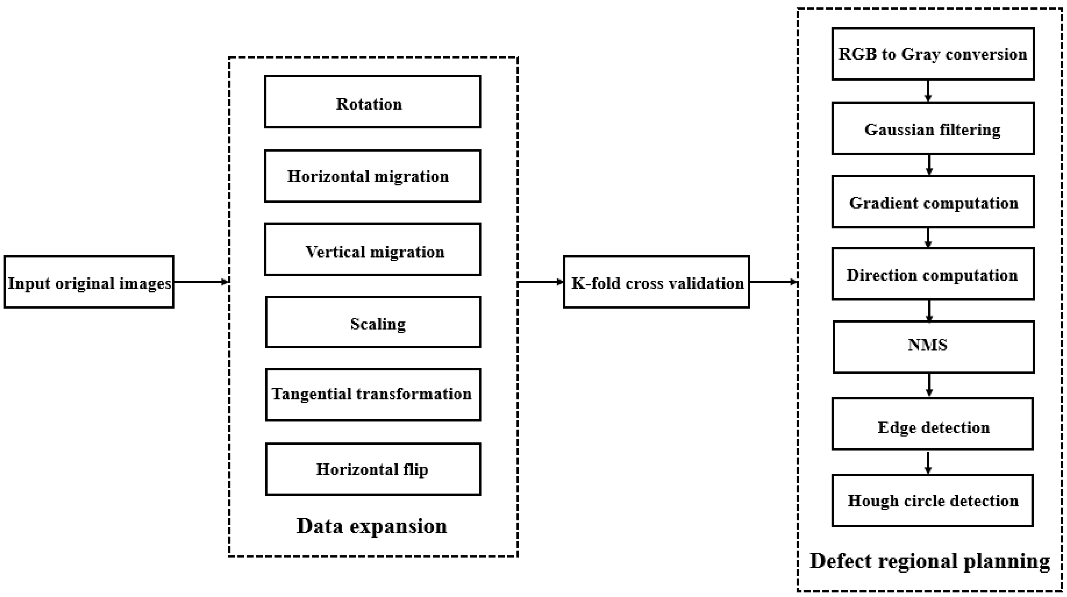
There are two purposes of image pre-processing: one is to enhance image quality to ensure sharp contrast and filter out noise, such as adopting histogram equalization and gray scale transformation to enhance contrast, or adopting methods such as median filtering and adaptive filtering to remove noise. The second is to segment the image to facilitate subsequent feature extraction, such as threshold segmentation, edge segmentation and region segmentation. In this paper, data enhancement and defect area planning were carried out in view of the features of a container mouth in a filling line, such as stability, monotonous shape and a limited number of images. The pre-processing flow is illustrated in Figure 1.

2.1.1. Data Enhancement

The defect images on the sealing surface of a container in the filling line were collected by a CCD camera. A total of 400 images were taken, covering defects like breaches, dents, burrs and abrasions. The images were converted to the size of 300 × 300 as the training inputs. Such a size can reduce the computing load in training without losing too much information from the images. Then, data expansion was performed to increase the number of images and prepare the dataset for K-fold cross-validation. During data expansion, the following actions were targeted: rotation, horizontal migration, vertical migration, scaling, tangential transformation and horizontal flip. In this way, the CNN could learn more invariant image features and prevent over-fitting. The implementation method of data expansion is shown in

Table 1. The implementation method of data expansion.

Data Expansion Mode	Changes
Rotation	From 0° to 10° random rotation of images
Horizontal migration	Horizontal migration images, and the offset value is 10% of the length of the images
Vertical migration	Vertical migration images, and the offset value is 10% of the length of the images
Scaling	Enlarge the images to 10% scale
Tangential transformation	Stretch the pixel points horizontally. The stretch value is 10% of the pixel points to the vertical axis distance
Horizontal flip	The images are randomly inverted with a horizontal axis as the symmetry axis

:

The K-fold cross validation method divides the expanded dataset C into K discrete subsets. During network training, a subset was selected as the test set, while the rest (K-1) subsets were combined into the training set. Each training outputs a classification accuracy of the network model on the selected test set. The same process was repeated K times to get the mean accuracy, i.e., the true accuracy of the model.

2.1.2. Defect Area Planning

The defect samples contain lots of useless background information that may affect the recognition quality of the detection algorithms. Our defect samples carry the following features: the defects concentrated on the sealing surface, whose round shape remains unchanged. In view of these, the Hough circle detection was used in the pre-processing phase to locate the edge of the cover, and mitigate the impact of useless background on the recognition accuracy. The Hough circle transform begins with the extraction of edge location and direction with a Canny operator. The Canny operation involves six steps: RGB to gray conversion, Gaussian filtering, gradient and direction computation, non-maximum suppression (NMS), double threshold selection and edge detection. Among them, Gaussian filtering is realized by the two-dimensional (2D) Gaussian kernel convolution:

$$\mathrm{K}=\frac{1}{2\mathsf{\pi }{\sigma }^2}{\mathrm{e}}^{-\frac{x^2+y^2}{2{\sigma }^2}}$$

(1)

The purpose of Gaussian filtering is to smoothen the image and remove as much noise as possible. Then, the Sobel operator was introduced to obtain the gradient amplitude and its direction, which can enhance the image and highlight the points with significant changes in neighboring pixels. The operator contains two groups of 3 × 3 kernels. One group is transverse detection kernels, and the other is vertical detection kernels. The formula of the operator is as follows:

$${\mathrm{G}}_{\mathrm{x}}=\left[\begin{array}{ccc}-1& 0& +1\\ -2& 0& +2\\ -1& 0& +1\end{array}\right]*\mathrm{A},{\mathrm{G}}_{\mathrm{y}}=\left[\begin{array}{ccc}+1& +2& +1\\ 0& 0& 0\\ -1& -2& -1\end{array}\right]*\mathrm{A}$$

(2)

where A is a smooth image; G_x is an image after transverse gradient detection; and G_y is an image after vertical gradient detection. The gradient can be expressed as:

$$\left|\nabla f\right|=\mathrm{mag}\left(\nabla f\right)={\left[{(\frac{\partial f}{\partial x})}^2+{(\frac{\partial f}{\partial y})}^2\right]}^{1/2}$$

(3)

The gradient direction can be expressed as:

$$\mathrm{a}(x,y)=\arctan (\frac{{\mathrm{G}}_y}{{\mathrm{G}}_x})$$

(4)

During edge detection, the NMS was adopted to find the maximum gradient of local pixels by comparing the gradients and gradient directions. After obtaining the binary edge image, the Hough circle transform was employed to detect the circles. Under the coordinate system $({\mathrm{c}}_1,{\mathrm{c}}_2,\mathrm{r})$, the formula of Hough circle transform can be described as:

$$(x{-\mathrm{c}}_1{)}^2+{\left(y{-\mathrm{c}}_2\right)}^2{=\mathrm{r}}^2$$

(5)

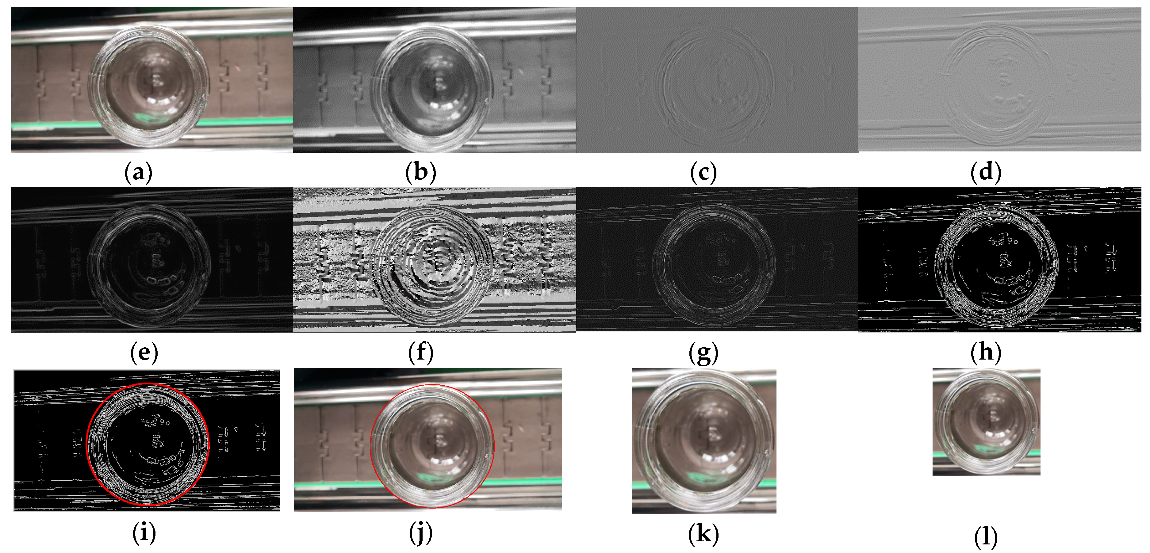
where $({\mathrm{c}}_1,{\mathrm{c}}_2)$ is the center of the center coordinates; and $\mathrm{r}$ is the radius. The detection was realized through the following steps: first, the non-zero points in the image are traversed, and line segments along the gradient direction (radius direction) and the opposite direction are drawn. The intersection point of the segments is the circle center. Then, the maximum circle is obtained by setting the threshold value. After that, the rectangular regions are generated by the maximum radius. The size of the image was normalized to 300 × 300 × 3. Figure 2 shows the regional planning process.

2.2. Defect Detection Model Based on MobileNet-SSD Network

2.2.1. Principles of MobileNet Feature Extraction

The MobileNet network [27] was developed to improve the real-time performance of deep learning under limited hardware conditions. This network can reduce the number of parameters without sacrificing accuracy. Previous studies have shown that MobileNet only needs 1/33 of the parameters of Visual geometry group -16 (VGG-16) to achieve the same classification accuracy in ImageNet-1000 classification tasks.

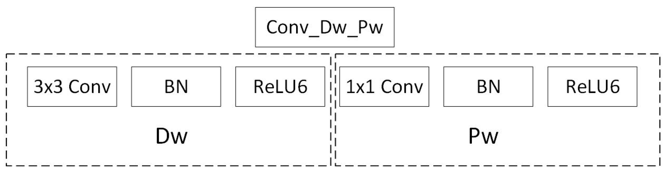
Figure 3 shows the basic convolution structure of MobileNet. Conv_Dw_Pw is a deep and separable convolution structure. It is composed of depth-wise layers (Dw) and point-wise layers (Pw). The Dw are deep convolutional layers using 3 × 3 kernels, while the Pw are common convolutional layers using 1 × 1 kernels. Each convolution result is treated by the batch normalization algorithm and the activation function rectified liner unit (ReLU).

In this paper, the activation function ReLU is replaced by ReLU6, and the normalization is carried out by the batch normalization (BN) algorithm, which supports the automatic adjustment of data distribution. The ReLU6 activation function can be expressed as:

$$y=\min {\displaystyle (}\max {\displaystyle (}z,0{\displaystyle )},6{\displaystyle )}$$

(6)

where z is the value of each pixel in the feature map.

The deep and separable convolutional structure enables the MobileNet to speed up the training and greatly reduces the amount of calculation. The reasons are as follows:

The standard convolution structure can be expressed as:

$${\mathrm{G}}_{\mathrm{N}}={\displaystyle \sum _{\mathrm{M}}{\mathrm{K}}_{\mathrm{M},\mathrm{N}}*{\mathrm{F}}_{\mathrm{M}}}$$

(7)

where ${\mathrm{K}}_{\mathrm{M},\mathrm{N}}$ is the filter; and M and N are respectively the number of input channels and output channels. During the standard convolution, the input image, including the feature image, ${\mathrm{F}}_{\mathrm{M}}$ means input images, including feature maps, which use the fill style of zero padding.

When the size and channels of input images respectively are ${\mathrm{D}}_{\mathrm{F}}{*\mathrm{D}}_{\mathrm{F}}$ and M, it is necessary to have N filters with M channels and the size of ${\mathrm{D}}_{\mathrm{K}}{*\mathrm{D}}_{\mathrm{K}}$ before outputting N feature images of the size ${\mathrm{D}}_{\mathrm{K}}{*\mathrm{D}}_{\mathrm{K}}$. The computing cost is ${\mathrm{D}}_{\mathrm{K}}{*\mathrm{D}}_{\mathrm{K}}{*\mathrm{M}*\mathrm{N}*\mathrm{D}}_{\mathrm{F}}{*\mathrm{D}}_{\mathrm{F}}$.

By contrast, the Dw formula can be expressed as:

$${\hat{\mathrm{G}}}_{\mathrm{M}}={\displaystyle \sum {\hat{\mathrm{K}}}_{1,\mathrm{M}}{*\mathrm{F}}_{\mathrm{M}}}$$

(8)

where ${\hat{\mathrm{K}}}_{1,\mathrm{M}}$ is the filter. ${\mathrm{F}}_{\mathrm{M}}$ has the same meaning as Formula (7). When the step size is one, the filling of zero ensures that the size of the characteristic graph is invariable after the application of deep and separable convolutional structure. When the step size is two, zero filling ensures that the size of the feature graph obtained after the application of deep and separable convolutional structure becomes half of the input image/feature graph; that is, the dimensional reduction operation is realized.

The deep separable convolution structure of MobileNet can obtain the same outputs as those of standard convolution based on the same inputs. The Dw phase needs M filters with one channel and the size of ${\mathrm{D}}_{\mathrm{K}}{*\mathrm{D}}_{\mathrm{K}}$. The Pw phase needs N filters with M channels and the size of 1 × 1. In this case, the computing cost of the deep separable convolution structure is ${\mathrm{D}}_{\mathrm{K}}{*\mathrm{D}}_{\mathrm{K}}{*\mathrm{M}*\mathrm{D}}_{\mathrm{F}}{*\mathrm{D}}_{\mathrm{F}}{+\mathrm{M}*\mathrm{N}*\mathrm{D}}_{\mathrm{F}}{*\mathrm{D}}_{\mathrm{F}}$, about $\frac{1}{\mathrm{N}}+\frac{1}{{\mathrm{D}}_{\mathrm{K}}^2}$ of that of standard convolution.

Besides, the data distribution will be changed by each convolution layer during network training. If the data are on the edge of the activation function, the gradient will disappear and the parameters will no longer be updated. Similar to the standard normal distribution, the BN algorithm adjusts the data by setting two learning parameters, and prevents gradient disappearance and the adjustment of complex parameters (e.g., learning rate and dropout ratio).

2.2.2. SSD Meta Structure

SSD network is a regression model, which uses features of different convolution layers to make classify regression and boundary box regression. The model solves the conflict between translation invariance and variability, and achieves good detection precision and speed.

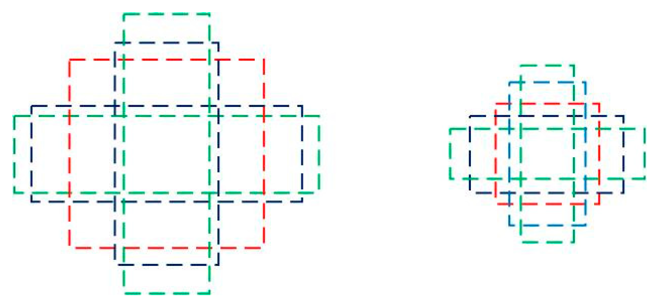
In each selected feature map, there are K frames that differ in size and width-to-height ratio. These frames are called the default boxes. Figure 4 expresses default boxes on feature maps of different convolutional layers. Each default box predicts the B class score and the four position parameters. Hence, $\mathrm{B}*\mathrm{k}*\mathrm{w}*\mathrm{h}$ class score and $4*\mathrm{k}*\mathrm{w}*\mathrm{h}$ position parameters must be predicted for a $\mathrm{w}*\mathrm{h}$ feature image. This requires $(\mathrm{B}+4)*\mathrm{k}*\mathrm{w}*\mathrm{h}$ convolution kernels of the size 3 × 3 to process the feature map. Then, the convolution results should be taken as the final feature for classification regression and bounding box regression. Here, B is set to four because there are four typical defects on the sealing surface of a container in the filling line. The scale of the default boxes for each feature map is computed as:

$${\mathrm{S}}_{\mathrm{k}}{=\mathrm{S}}_{\min }+\frac{{\mathrm{S}}_{\max }{-\mathrm{S}}_{\min }}{\mathrm{m}-1}(\mathrm{k}-1),(\mathrm{k}\in [1,\mathrm{m}])$$

(9)

where m is the number of feature maps; and ${\mathrm{S}}_{\max }$, ${\mathrm{S}}_{\min }$ are parameters that can be set. In order to control the fairness of feature vectors in the training and test experiments, the same five kinds of width-to-height ratios $a_r=\{1,2,3,0.5,0.33\}$ were used to generate default boxes. Then, each default box can be described as:

$$\begin{gathered} {\mathrm{w}}_{\mathrm{k}}^{\mathrm{a}}{=\mathrm{S}}_{\mathrm{k}}\sqrt{{\mathrm{a}}_{\mathrm{r}}} \\ {\mathrm{h}}_{\mathrm{k}}^{\mathrm{a}}{=\mathrm{S}}_{\mathrm{k}}/\sqrt{{\mathrm{a}}_{\mathrm{r}}} \end{gathered}$$

(10)

where ${\mathrm{w}}_{\mathrm{k}}^{\mathrm{a}}$ is the width of default boxes; and ${\mathrm{h}}_{\mathrm{k}}^{\mathrm{a}}$ is the height of default boxes.

Next, a default box ${\mathrm{S}}_{\mathrm{k}}^{\prime }=\sqrt{{\mathrm{S}}_{\mathrm{k}}{\mathrm{S}}_{\mathrm{k}+1}}$ should be added when the width-to-height ratio is one. The center of each default box is $(\frac{\mathrm{i}+0.5}{\left|{\mathrm{f}}_{\mathrm{k}}\right|},\frac{\mathrm{j}+0.5}{\left|{\mathrm{f}}_{\mathrm{k}}\right|})$, and $\left|{\mathrm{f}}_{\mathrm{k}}\right|$ is the size of the K-th feature unit, $\mathrm{i},\mathrm{j}\in [0,\left|{\mathrm{f}}_{\mathrm{k}}\right|]$. The intersection over union (IoU) between area A and area B can be calculated as:

$$\mathrm{IoU}=\frac{\mathrm{area}\left(\mathrm{A}\right)\cap \mathrm{area}\left(\mathrm{B}\right)}{\mathrm{area}\left(\mathrm{A}\right)\cup \mathrm{area}\left(\mathrm{B}\right)}$$

(11)

If the IoU of default box and calibration box (Ground-truth Box) is greater than 0.5, it means the default box matches the calibration box of that category.

The SSD is an end-to-end training model. The overall loss function of the training contains the confidence loss ${\mathrm{L}}_{\mathrm{conf}}\left(\mathrm{s},\mathrm{c}\right)$ of the classification regression and the position loss of the bounding box regression ${\mathrm{L}}_{\mathrm{loc}}\left(\mathrm{r},\mathrm{l},\mathrm{g}\right)$. This function can be described as:

$$\mathrm{L}{\displaystyle (}\mathrm{s},\mathrm{r},\mathrm{c},\mathrm{l},\mathrm{g}{\displaystyle )}=\frac{1}{\mathrm{N}}{\displaystyle (}{\mathrm{L}}_{\mathrm{conf}}{\displaystyle (}\mathrm{s},\mathrm{c}{\displaystyle )}{+\mathsf{\alpha }\mathrm{L}}_{\mathrm{loc}}{\displaystyle (}\mathrm{r},\mathrm{l},\mathrm{g}{\displaystyle )}{\displaystyle )}$$

(12)

where $\mathsf{\alpha }$ is a parameter to balance the confidence loss and position loss; s and r are the eigenvectors of confident loss and position loss, respectively; c is the classification confidence; l is the offset of predicted box, including the translation offset of the center coordinate and scaling offset of the height and width; g is the calibration box of the target actual position; and N is the number of default boxes that match the calibration boxes of this category.

2.2.3. Surface Defect Detection Algorithm Based on MobileNet-SSD Model

In the filling line, the sealing surface is easily damaged by friction, collision and extrusion in the recycling and transport of pressure vessels. The common defects include breaches, dents, burrs and abrasions on the sealing surface. In this paper, the MobileNet-SSD model can greatly reduce the number of parameters, and achieve higher accuracy under the limited hardware conditions. The complete model contains four parts: the input layer for importing the target image, the MobileNet base net for extracting image features, the SSD for classification regression and bounded box regression and the output layer for exporting the detection results.

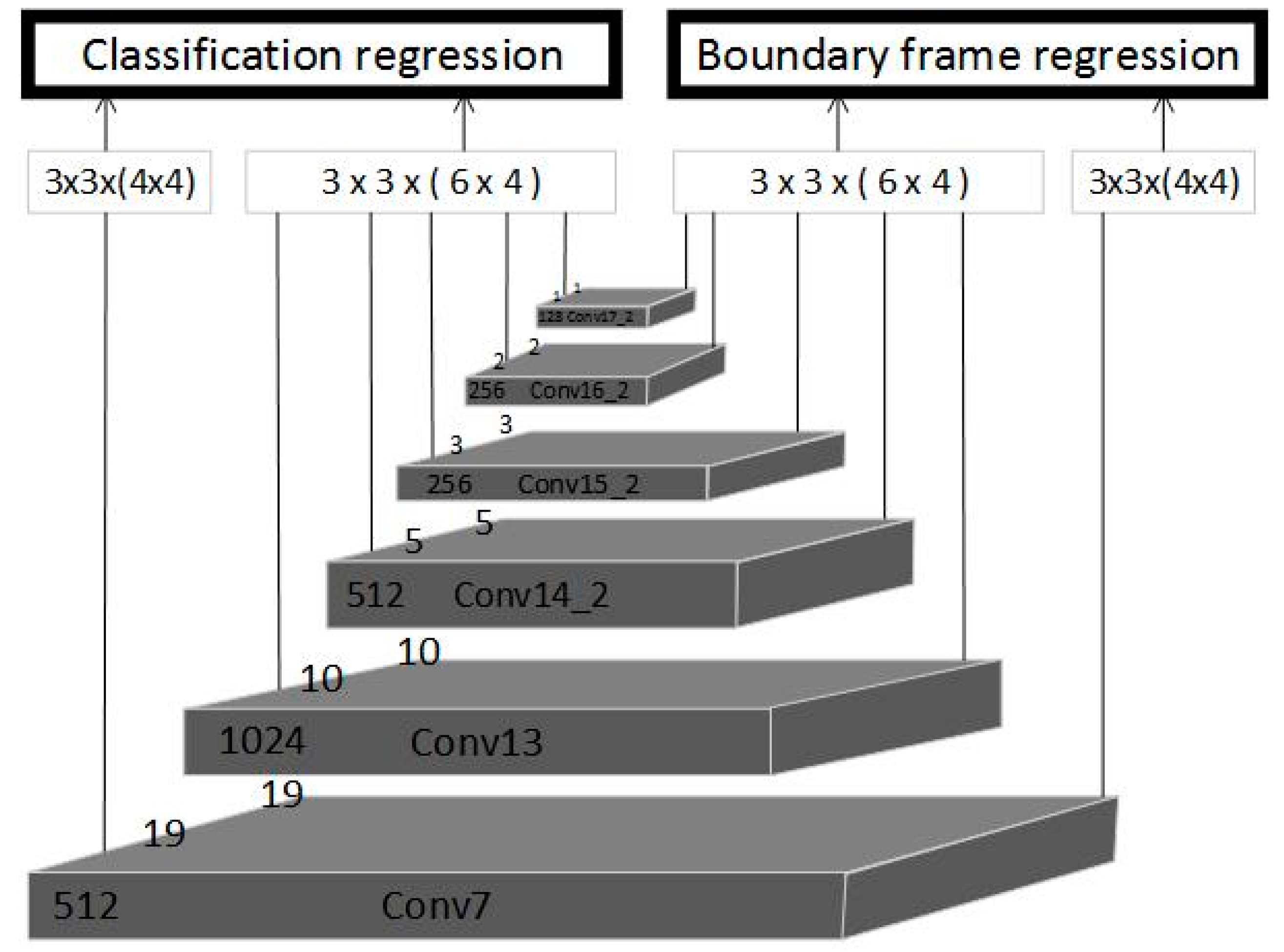
This model supports fast and accurate detection because the structure of MobileNet reduces the complexity of computing. However, the structure of Pw changes the distribution of output data of Dw. This may cause a loss of precision. To solve this problem, the fully-connected layers were abandoned, and eight standard convolutional layers were added with the aim to widen the receptive field of the feature image, adjust the data distribution and enhance the translation invariance of the classification task. To prevent the disappearance of the gradient, the BN layer and activation function ReLU6 were introduced to each layer of the added structure. In addition, the two-layer feature image in MobileNet and the four-layer feature image in the added standard convolutional layers constituted a feature image pyramid (Figure 5). Kernels 3 × 3 in size were adopted as the convolutional kernels to convolve selected feature maps. The convolutional results were taken as the final feature for classification regression and bounded box regression.

A 300 × 300 image was taken as the input. The six layers of the pyramid respectively contain 4, 6, 6, 6, 6 and 6 default boxes. Besides, different 3 × 3 kernels were adopted for classification and location with the step length of one. The numbers in brackets were the amount of 3 × 3 filters that are applied around each location in the feature map. Its number was the amount of default Box × number of categories (classification) and the amount of default Box × 4(location), respectively. The general structure of MobileNet-SSD is shown in

Table 2. General structure of MobileNet-SSD. ※ = the feature image to be used in classification regression and bounded box regression.

Convolution	Step	Input	Output
Conv0_BN_ReLU6(3 × 3)	2	3	32
Conv1_Dw_Pw(3 × 3)	Dw:1	32	64
Conv2_Dw_Pw(3 × 3)	Dw:2	64	128
Conv3_Dw_Pw(3 × 3)	Dw:1	128	128
Conv4_Dw_Pw(3 × 3)	Dw:2	128	256
Conv5_Dw_Pw(3 × 3)	Dw:1	256	256
Conv6_Dw_Pw(3 × 3)	Dw:2	256	512
※Conv7_Dw_Pw(3 × 3)	Dw:1	512	512
Conv8_Dw_Pw(3 × 3)	Dw:1	512	512
Conv9_Dw_Pw(3 × 3)	Dw:1	512	512
Conv10_Dw_Pw(3 × 3)	Dw:1	512	512
Conv11_Dw_Pw(3 × 3)	Dw:1	512	512
Conv12_Dw_Pw(3 × 3)	Dw:2	512	1024
※Conv13_Dw_Pw(3 × 3)	Dw:1	1024	1024
Conv14_1_BN_ReLU6(1 × 1)	1	1024	256
※Conv14_2_BN_ReLU6(3 × 3)	2	256	512
Conv15_1_BN_ReLU6(1 × 1)	1	512	128
※Conv15_2_BN_ReLU6(3 × 3)	2	128	256
Conv16_1_BN_ReLU6(1x1)	1	256	128
※Conv16_2_BN_ReLU6(3 × 3)	2	128	256
Conv17_1_BN_ReLU6(1 × 1)	1	256	64
※Conv17_2_BN_ReLU6(3 × 3)	2	64	128

.

In Table 2, Conv_BN_ReLU6 is a standard convolutional layer, while Conv1_Dw_Pw is a deep and separable convolutional layer. Besides, the sign ※ represents the feature image to be used in classification regression and bounded box regression. Considering the small size of the target defects, the feature image of the shallow Conv7_Dw_Pw output was adopted for further analysis.

3. Experimental Results and Analysis

Our experiment targets an oil chili filling production line in China’s Guizhou Province. During the detection, the image of the sealing surface was transmitted via the image acquisition unit to the host for image signal processing. Then, the corresponding features were extracted and the defects were detected and marked by the MobileNet-SSD network. Specifically, the MobileNet-SSD served as the training base net of the pre-processed database; then, the trained model was migrated to the detection network for boundary box regression and classification regression. A total of five width-to-height ratios were selected according to the defect size, namely, 1, 2, 3, 0.5 and 0.33 respectively. The $S_{\max }$ was set to 0.95 and the $S_{\min }$ to 0.2. The six layers of the pyramid respectively contain 4, 6, 6, 6, 6 and 6 default boxes. During the training, the IoU of the positive sample fell in (0.5, 1), that of the negative sample fell in (0.2, 0.5), and the difficulty of the sample fell in (0, 0.2). In addition, the learning rate of this paper is the exponential decay learning rate initialized to 0.1, and random initialization weights and bias terms.

3.1. Image Processing Unit

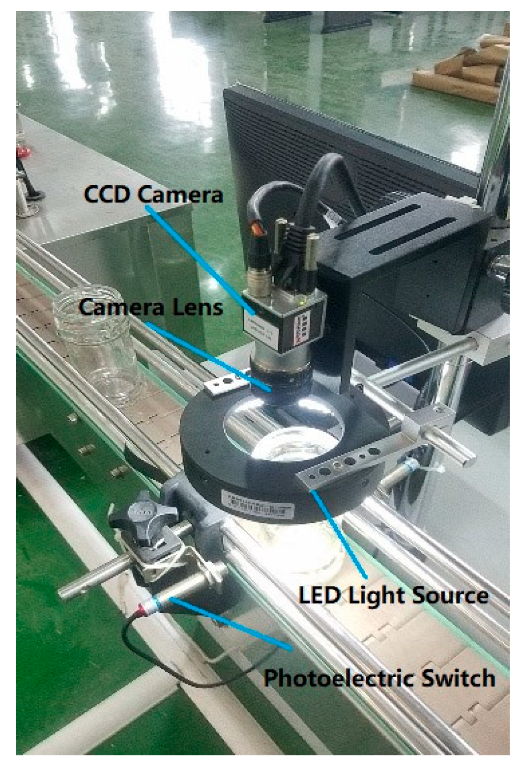
As shown in Figure 6, the image acquisition unit consists of a transmission mechanism, a proximity switch sensor, an industrial CCD camera, a light-emitting diode (LED) arc light source and a lens. Before the acquisition, the LED arc light source was adjusted to calibrate the brightness, and the lens was mounted on the CCD camera. Then, the aperture and focal length were adjusted to ensure the imaging quality of the acquisition unit. Under the action of the transmission mechanism, the sensor detected the workpiece and produced pulse signals when the vessel maintained a constant speed and spacing. These signals triggered the CCD camera to take photos. In order to ensure that the container runs to the center of view field, sensor needs to be accurately debugged.

The detection network was trained on the following hardware: Intel Core i7 7700K processor (Vietnam, 2017) which has a main frequency of 4.2 GHz, 32 GB memory and a GeForce TITAN X graphics processing unit (GPU). The software part used the Ubuntu 14.04.2 operating system, and the Tensorflow deep learning framework. Twenty percent of the samples in the pre-processed library were allocated to the test set and the other 80% to the training set.

3.2. Comparison of Three Deep Learning Networks

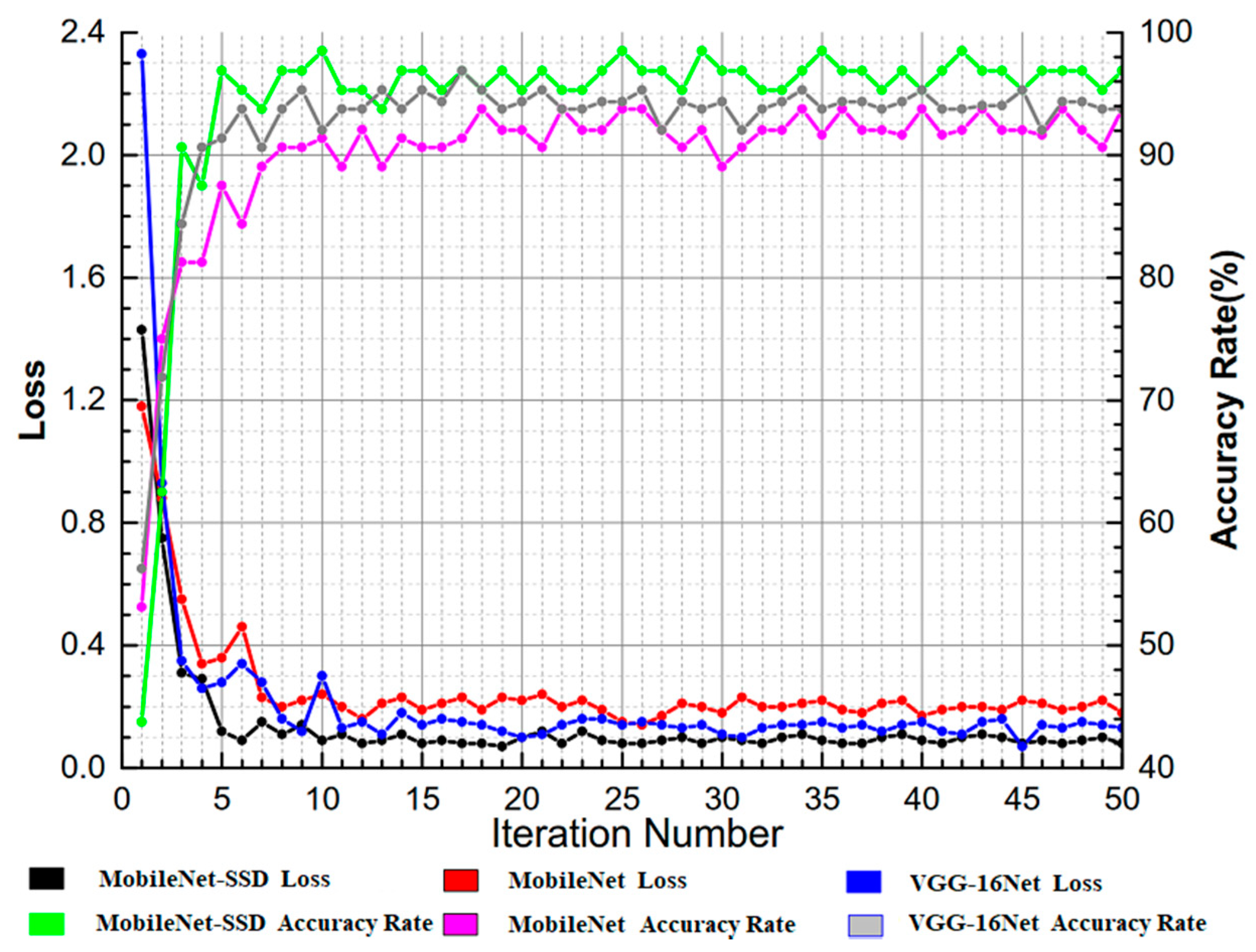
The loss function and the accuracy of the proposed MobileNet-SSD surface defect detection algorithm on the test set (Figure 7) were compared to those of the VGGNet [28], an excellent detection network in 2014 ImageNet and MobileNet. The three algorithms were trained via migration learning and data enhancement. The training parameters and results are shown in

Table 3. Training parameters and results of the three detection networks. SGD = stochastic gradient descent.

Parameter	VGG-16	MobileNet	MobileNet-SSD
Basic learning rate	0.003	0.003	0.003
Number of iterations of training	10,000	10,000	10,000
Verifying the number of iterations	50	50	50
Batch quantity	128	128	128
Optimization algorithm	SGD	SGD	SGD
Network parameter (million)	≈12.30	≈1.76	≈1.92
Amount of calculation (million)	≈1325.00	≈127.54	≈157.32
Mean of loss function	0.14	0.19	0.09
Mean value (%)	93.91	92.33	96.73

.

In the training process, the detection networks were tested once after two hundred iterations of the training set. The loss function and accuracy in Table 2 were mean values obtained from 40 to 50 iterations of the test set. It is clear that the MobileNet-SSD detection algorithm achieved better accuracy than the other two networks with fewer network parameters.

3.3. Results of Defect Detection Network

The trained network parameters were adopted for the MobileNet-SSD defect detection network. The test set image contained four different types of defect samples, each of which had 30 images obtained through resampling. Each sample involved one or more defects. The detection results of the trained MobileNet-SSD defect detection network on the four kinds of defect samples are show in

Table 4. Detection results of the trained MobileNet-SSD algorithm.

Defect Type	Sample Number	Successful Detection Number	Leakage Number	Error Detection Number	Positive Rate (%)
Breach	30	30	0	0	100.00
Dent	30	27	2	1	90.00
Burr	30	28	1	1	93.33
Abrasion	30	39	1	0	96.67
Total	120	115	4	2	95.00

.

It can be seen from Table 3 that the surface defect detection network completes the defect marking of 120 defect samples with a 95.00% accuracy rate. There were missing and false samples in dent and burr defects and missing samples in abrasion defects. This is because the notches are more obvious than the other defects, and related to the image quality and subjective feelings of humans.

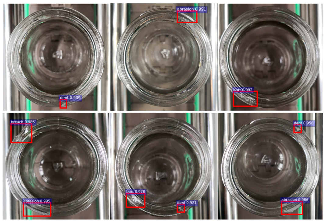
When the filling line was in operation, the container passed by the image acquisition device within a certain distance, triggering the CCD camera to take photos. The defect detection network performed forward operation. If there were defects in the image, the alarm would buzz and the defect type and location were identified by the host (Figure 8). The single forward operation of the network was at the rate of 0.12 s/image.

3.4. Degree of Defect Detection

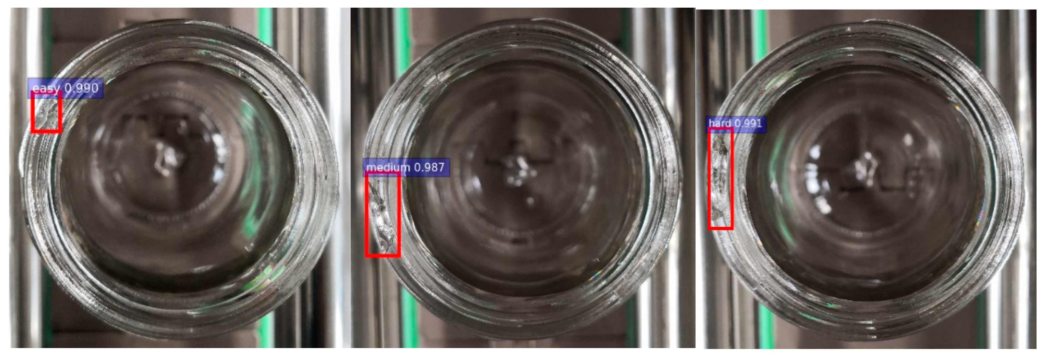
The defects of the same type may differ in terms of severity. Here, the pre-processed datasets were divided into three categories based on the defect severity: easy, medium and hard. The recognition result can serve as a yardstick of the network classification quality. Seventy percent of all samples were divided into the training set and the remaining 30% to the test set. The detection results of the breaches are shown in Figure 9.

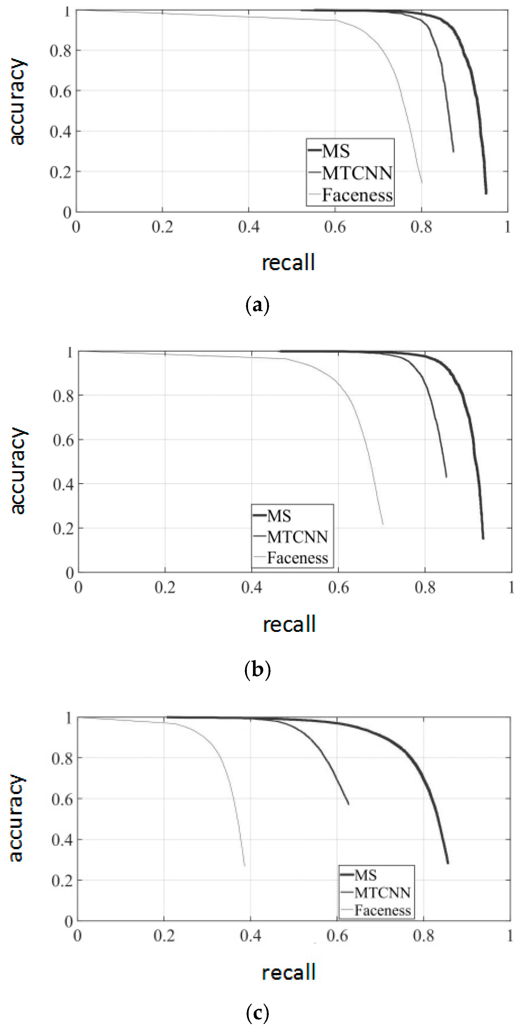
Figure 10 shows the precision–recall (PR) curves of the experimental dataset. The advanced multi-task CNN (MTCNN) [29] and Faceness-Net [30] were contrasted with the proposed MobileNet-SSD algorithm (“MS” in the figure) on the experimental dataset. The experimental results show that the recall rates of the proposed algorithm were 93.11%, 92.18% and 82.97%, in easy, medium and hard subsets, respectively, and its performance was better than that of the contrastive algorithms.

3.5. Contrast Experiment

Three comparative experiments were designed to further validate the proposed algorithm. In the first experiment, the proposed algorithm was compared to five lightweight feature extraction networks, including SqueezeNet [31], MobileNet, performance vs accuracy net (PVANet) [32], MTCNN and Faceness-Net. The feature extraction accuracy of each algorithm for the ImageNet classification task is displayed in

Table 5. Feature extraction accuracy of each algorithm. GFLOPS =floating-point operations per second. GPU = graphics processing unit. PVANet= performance vs accuracy net.

Model	Top-1	Top-5	GFLOPS	GPU
SqueezeNet	57.64	80.40	0.858	700 ms
MTCNN	63.85	85.03	0.897	640 ms
MobileNet	69.37	89.22	0.513	610 ms
Faceness-Net	70.31	84.39	0.858	720 ms
PVANet	72.43	90.16	0.606	150 ms
MobileNet-SSD	81.26	94.62	0.812	120 ms

. In the second experiment, the above five networks were contrasted with the proposed algorithm in defect detection of the filling line in terms of correct detection rate, training time and the detection time per image (

Table 6. Correct detection rate, training time and the detection time per image of each network.

Number	Model	Positive Rate	Training Time (Day)	Detection Time (s)
1	SqueezeNet	85.83%	2	0.31
2	Faceness-Net	90.83%	3	0.59
3	MobileNet	90.83%	<1	0.54
4	MTCNN	91.67%	3	0.64
5	PVANet	94.17%	2	0.25
6	MobileNet-SSD	95.00%	<1	0.12

).

As shown in the two tables, the MobileNet-SSD surface defect model is fast and stable, thanks to the improved SSD meta-structure of the feature pyramid. In general, the proposed algorithm outperformed the contrastive algorithms in detection rate, training time and detection time. The final detection time of our algorithm was merely 120 milliseconds per piece, which meets the real-time requirements of the industrial filling line.

In Contrast Experiment 3, four traditional defect recognition methods of k-nearest neighbor (KNN) [33], HMM [34,35,36], SVM and HMM [37] and back propagation neural network (BPNN) [38] are realized, which are compared with the method in this paper. The KNN method selects Euclidean distance as the distance function; the HMM model adopts a sampling window of 5 × 4 size and uses the discrete cosine transform (DCT) coefficient as the observation vector of HMM. The SVM and HMM method is the same as in literature [37]. The hidden layer number of the BP neural network is set to 30. The above models are also applied to detect the defects on the sealing surface of a container in the filling line. The statistical results are shown in

Table 7. Correct detection rate and the detection time per image of each model. HMM: Hidden Markov Model. SVM = support vector machine. KNN = k-nearest neighbor. BPNN = back propagation neural network.

Number	Model	Positive Rate	Detection Time (s)
1	KNN	65.83%	0.31
2	HMM	66.67%	0.39
3	SVM and HMM	80.83%	0.32
4	BPNN	84.17%	0.14
5	MobileNet-SSD	95.00%	0.12

.

As can be seen from Table 6, compared with the other traditional defect detection methods, the MobileNet-SSD method has a higher positive detection rate. Under the same hardware conditions, MobileNet-SSD still maintains the optimal speed despite the small differences between the above five methods. In addition, the results of HMM and KNN are not ideal. The reason for this may be that the proportion of defects is small, and the sealing surface of a container contains a lot of background information. KNN and HMM did not extract specific features of the image before classifying. However, both the BP neural network and MobileNet-SSD are based on neural networks, which can automatically learn features by itself, so the accuracy rate of the two methods are relatively high. MobileNet-SSD, due to its unique deep convolutional structure, can learn the deep and detachable features of defects with a bigger receptive field, so it can achieve a higher positive detection rate.

4. Conclusions

This paper proposes a surface defect detection method based on the MobileNet-SSD network, and applies it to identify the types and locations of surface defects. In the pre-processing phase, a regional planning method was presented to cut out the main body of the defect, reduce redundant parameters and improve detection speed and accuracy. Meanwhile, the robustness of the algorithm was elevated by data enhancement. The philosophy of MobileNet, a lightweight network, was introduced to enhance the detection accuracy, reduce the computing load and shorten the training time of this algorithm. The MobileNet and SSD were adjusted to detect the surface defects, such that the proposed method could differentiate small defects from the background. The feasibility of the proposed method was verified by defect detection for the sealing surface of an oil chili filling production line in Guizhou, China. Specifically, an image acquisition device was established for the sealing surface and the deep learning framework was adopted to mark the defect positions. The results show that the proposed method can identify most defects in the production environment at high speed with accuracy. However, the system also has its limitations. Deep learning models have a certain dependence on the hardware platform because of computationally intensive processes, and they are not suitable for embedded systems with general performance. Future research will further improve the proposed method through integration with embedded chips and the Internet of Things, balancing the classification accuracy and number of parameters of the detection method, and expand the application scope of our method to complex defects in industrial processes.

References

- Uddin, M.T.; Uddiny, M.A. Human activity recognition from wearable sensors using extremely randomized trees. In Proceedings of the International Conference on Electrical Engineering and Information Communication Technology, Dhaka, Bangladesh, 21–23 May 2015; pp. 1–6. [Google Scholar]
- Jalal, A.; Sarif, N.; Kim, J.T.; Kim, T.S. Human Activity Recognition via Recognized Body Parts of Human Depth Silhouettes for Residents Monitoring Services at Smart Home. Indoor Built Environ. 2013, 22, 271–279. [Google Scholar] [CrossRef]
- Zhan, Y.; Kuroda, T. Wearable sensor-based human activity recognition from environmental background sounds. J. Ambient Intell. Hum. Comput. 2014, 5, 77–89. [Google Scholar] [CrossRef]
- Jalal, A. Security Architecture for Third Generation (3G) using GMHS Cellular Network. In Proceedings of the International Conference on Emerging Technologies, Islamabad, Pakistan, 12–13 November 2008; pp. 74–79. [Google Scholar]
- Shire, A.N.; Khanapurkar, M.M.; Mundewadikar, R.S. Plain Ceramic Tiles Surface Defect Detection Using Image Processing. In Proceedings of the International Conference on Emerging Trends in Engineering and Technology, Port Louis, Mauritius, 18–20 November 2012; pp. 215–220. [Google Scholar]
- Shang, L.; Yang, Q.; Wang, J.; Li, S.; Lei, W. Detection of rail surface defects based on CNN image recognition and classification. In Proceedings of the International Conference on Advanced Communication Technology, Chuncheon-si, Korea, 11–14 February 2018; pp. 45–51. [Google Scholar]
- Jalal, A.; Kim, S. Advanced Performance Achievement using Multi-Algorithmic Approach of Video Transcoder for Low Bitrate Wireless Communication. ICGST Int. J. Graph. Vis. Image Process. 2004, 5, 27–32. [Google Scholar]
- Deutschl, E.; Gasser, C.; Niel, A.; Werschonig, J. Defect detection on rail surfaces by a vision based system. In Proceedings of the Intelligent Vehicles Symposium, Parma, Italy, 14–17 June 2004; pp. 507–511. [Google Scholar]
- Yazdchi, M.; Yazdi, M.; Mahyari, A.G. Steel Surface Defect Detection Using Texture Segmentation Based on Multifractal Dimension. In Proceedings of the International Conference on Digital Image Processing, Bangkok, Thailand, 7–9 March 2009; pp. 346–350. [Google Scholar]
- Kamal, S.; Jalal, A.; Kim, D. Depth Images-based Human Detection, Tracking and Activity Recognition Using Spatiotemporal Features and Modified HMM. J. Electr. Eng. Technol. 2016, 11, 1921–1926. [Google Scholar] [CrossRef]
- Jalal, A.; Kim, S. Global Security Using Human Face Understanding under Vision Ubiquitous Architecture System. World Acad. Sci. Eng. Technol. 2006, 13, 7–11. [Google Scholar]
- Patil, K.; Kulkarni, M.; Sriraman, A.; Karande, S. Deep Learning Based Car Damage Classification. In Proceedings of the IEEE International Conference on Machine Learning and Applications, Cancun, Mexico, 18–21 December 2017; pp. 50–54. [Google Scholar]
- Zhang, Z.; Alonzo, R.; Athitsos, V. Experiments with computer vision methods for hand detection. In Proceedings of the Petra 2011 International Conference on Pervasive Technologies Related to Assistive Environments, Crete, Greece, 25 May 2011; pp. 1–6. [Google Scholar]
- Jeon, Y.J.; Choi, D.C.; Lee, S.J.; Yun, J.P.; Kim, S.W. Steel-surface defect detection using a switching-lighting scheme. Appl. Opt. 2016, 55, 47–57. [Google Scholar] [CrossRef] [PubMed]
- Kabouri, A.; Khabbazi, A.; Youlal, H. Applied multiresolution analysis to infrared images for defects detection in materials. NDT E Int. 2017, 92, 38–49. [Google Scholar]
- Krummenacher, G.; Ong, C.S.; Koller, S.; Kobayashi, S.; Buhmann, J.M. Wheel Defect Detection with Machine Learning. IEEE Trans. Intell. Transp. Syst. 2018, 19, 1176–1187. [Google Scholar] [CrossRef]
- Fu, L.; Wang, Z.; Liu, C. Research on surface defect detection of ceramic ball based on fringe reflection. Opt. Eng. 2017, 56, 104104. [Google Scholar]
- Jian, C.; Gao, J.; Ao, Y. Automatic Surface Defect Detection for Mobile Phone Screen Glass Based on Machine Vision. Appl. Soft Comput. 2016, 52, 348–358. [Google Scholar] [CrossRef]
- Win, M.; Bushroa, A.R.; Hassan, M.A.; Hilman, N.M.; Ide-Ektessabi, A. A Contrast Adjustment Thresholding Method for Surface Defect Detection Based on Mesoscopy. IEEE Trans. Ind. Inform. 2017, 11, 642–649. [Google Scholar] [CrossRef]
- LeCun, Y.; Bengio, Y.; Hinton, G. Deep learning. Nature 2015, 521, 436–444. [Google Scholar] [CrossRef] [PubMed]
- Esteva, A.; Kuprel, B.; Novoa, R.A.; Ko, J.; Swetter, S.M.; Blau, H.M.; Thrun, S. Dermatologist-level classification of skin cancer with deep neural networks. Nature 2017, 542, 115–118. [Google Scholar] [CrossRef] [PubMed]
- Litjens, G.; Kooi, T.; Bejnordi, B.E.; Setio, A.A.; Ciompi, F.; Ghafoorian, M.; van der Laak, J.A.; Van Ginneken, B.; Sánchez, C.I. A survey on deep learning in medical image analysis. Med. Image Anal. 2017, 42, 60–88. [Google Scholar] [CrossRef] [PubMed] [Green Version]
- Xian-Bao, W.; Jie, L.; Ming-Hai, Y.; Wen-Xiu, H.; Yun-Tao, Q. Solar Cells Surface Defects Detection Based on Deep Learning. Pattern Recognit. Artif. Intell. 2014, 27, 517–523. [Google Scholar]
- Cha, Y.J.; Choi, W.; Büyüköztürk, O. Deep Learning-Based Crack Damage Detection Using Convolutional Neural Networks. Comput. Aided Civ. Infrastruct. Eng. 2017, 32, 361–378. [Google Scholar] [CrossRef]
- Han, K.; Sun, M.; Zhou, X.; Zhang, G.; Dang, H.; Liu, Z. A new method in wheel hub surface defect detection: Object detection algorithm based on deep learning. In Proceedings of the International Conference on Advanced Mechatronic Systems, Xiamen, China, 6–9 December 2017; pp. 335–338. [Google Scholar]
- Liu, W.; Anguelov, D.; Erhan, D.; Szegedy, C.; Reed, S.; Fu, C.Y.; Berg, A.C. SSD: Single Shot MultiBox Detector. In Proceedings of the European Conference on Computer Vision, Amsterdam, The Netherlands, 11–14 October 2016; pp. 21–37. [Google Scholar]
- Howard, A.G.; Zhu, M.; Chen, B.; Kalenichenko, D.; Wang, W.; Weyand, T.; Andreetto, M.; Adam, H. MobileNets: Efficient Convolutional Neural Networks for Mobile Vision Applications. arXiv, 2017; arXiv:1704.04861. [Google Scholar]
- Simonyan, K.; Zisserman, A. Very Deep Convolutional Networks for Large-Scale Image Recognition. arXiv, 2014; arXiv:1409.1556. [Google Scholar]
- Zhang, K.; Zhang, Z.; Li, Z.; Qiao, Y. Joint Face Detection and Alignment Using Multitask Cascaded Convolutional Networks. IEEE Signal Process. Lett. 2016, 23, 1499–1503. [Google Scholar] [CrossRef] [Green Version]
- Yang, S.; Luo, P.; Loy, C.C.; Tang, X. Faceness-Net: Face Detection through Deep Facial Part Responses. IEEE Trans. Pattern Anal. Mach. Intell. 2018, 40, 1845–1859. [Google Scholar] [CrossRef] [PubMed] [Green Version]
- Iandola, F.N.; Han, S.; Moskewicz, M.W.; Ashraf, K.; Dally, W.J.; Keutzer, K. SqueezeNet: AlexNet-level accuracy with 50 × fewer parameters and <0.5 MB model size. arXiv, 2016; arXiv:1602.07360. [Google Scholar]
- Hong, S.; Roh, B.; Kim, K.H.; Cheon, Y.; Park, M. PVANet: Lightweight Deep Neural Networks for Real-time Object Detection. arXiv, 2016; arXiv:1611.08588. [Google Scholar]
- Hunt, M.A.; Karnowski, T.P.; Kiest, C.; Villalobos, L. Optimizing automatic defect classification feature and classifier performance for post. In Proceedings of the 2000 IEEE/SEMI Advanced Semiconductor Manufacturing Conference and Workshop, Boston, MA, USA, 12–14 September 2000; pp. 116–123. [Google Scholar]
- Jalal, A.; Kamal, S.; Kim, D. A depth video sensor-based life-logging human activity recognition system for elderly care in smart indoor environments. Sensors 2014, 14, 11735–11759. [Google Scholar] [CrossRef] [PubMed]
- Jalal, A.; Kim, Y.H.; Kim, Y.J.; Kamal, S.; Kim, D. Robust human activity recognition from depth video using spatiotemporal multi-fused features. Pattern Recognit. 2017, 61, 295–308. [Google Scholar] [CrossRef]
- Jalal, A.; Kamal, S.; Kim, D. Individual detection-tracking-recognition using depth activity images. In Proceedings of the 2015 12th International Conference on IEEE Ubiquitous Robots and Ambient Intelligence (URAI), Goyang, Korea, 28–30 October 2015; pp. 450–455. [Google Scholar]
- Wu, H.; Pan, W.; Xiong, X.; Xu, S. Human activity recognition based on the combined svm&hmm. In Proceedings of the 2014 IEEE International Conference on Information and Automation (ICIA), Hailar, China, 28–30 July 2014; pp. 219–224. [Google Scholar]
- Islam, M.A.; Akhter, S.; Mursalin, T.E.; Amin, M.A. A suitable neural network to detect textile defects. In Proceedings of the International Conference on Neural Information Processing, Hong Kong, China, 3–6 October 2006; Springer: Berlin/Heidelberg, Germany, 2006; pp. 430–438. [Google Scholar]
Figure 1.
The flow of image pre-processing. NMS = non-maximum suppression.
Figure 2.
(a) Original image; (b) Gaussian smooth image; (c) X directional gradient graph; (d) Y directional gradient graph; (e) Amplitude image; (f) Angle image; (g) Non-maximum value suppression graph; (h) Edge detection chart; (i) Maximum circle detection; (j) Maximum circle position of the original graph; (k) Cutting; (l) Normalization.
Figure 3.
The basic convolutional structure of MobileNet. Dw = depth-wise layers. Pw = point-wise layers. BN = batch normalization. Conv = convolution. ReLU6 = rectified liner unit 6.
Figure 4.
Default boxes on feature maps.
Figure 5.
MobileNet-Single Shot MultiBox Detector (SSD) network feature pyramid.
Figure 6.
Image acquisition device. CCD = charge-coupled device. LED = light-emitting diode.
Figure 7.
Loss function and accuracy of the three detection networks. VGG = visual geometry group.
Figure 8.
Detection effect of sealing surface defects.
Figure 9.
Static image detection results of notches.
Figure 10.
(a) Easy precision–recall (PR) curves of three different algorithms; (b) Medium PR curves of three different algorithms; (c) Hard PR curves of three different algorithms. MS = MobileNet-SSD. MTCNN = multi-task convolution neural network.