Research of Feature Extraction Method Based on Sparse Reconstruction and Multiscale Dispersion Entropy


The State Key Lab of Fluid Power Transmission and Controls, Zhejiang University, No.38, Zheda Rd, Hangzhou 310027, China
*
Author to whom correspondence should be addressed.
Appl. Sci. 2018, 8(6), 888; https://doi.org/10.3390/app8060888
Submission received: 16 April 2018
/
Revised: 15 May 2018
/
Accepted: 24 May 2018
/
Published: 29 May 2018
(This article belongs to the Special Issue Fault Detection and Diagnosis in Mechatronics Systems)
Abstract
:As one of the most important components in rotating machinery, it’s necessary and essential to monitor the rolling bearing operating condition to prevent equipment failure or accidents. However, in vibration signal processing, the bearing initial fault detection under background noise is quite difficult. Therefore, in this paper a new feature extraction method combining sparse reconstruction and Multiscale Dispersion Entropy (MDErms) is proposed. Firstly, the Sliding Matrix Sequences (SMS) truncation and sparse reconstruction by Hankel-matrix are applied to the vibration signal. Then MDErms is utilized as a characteristic index of vibration signal, which is suitable for a short time series. Additionally, the MDErms is employed in the sparse reconstructed matrix sequences to achieve the Multiscale Fusion Entropy Value Sequence (MFEVS). The MFEVS keeps the fault potential feature information in different scales and is superior in distinguishing fault periodic impulses from heavy background noise. Finally, the designed FIR bandpass filter based on the MFEVS, shows prominent features in denoising and detecting weak bearing faults, which is separately verified by simulation studies and artificial fault experiments in different cases. By comparison with traditional methods like EEMD, Wavelet Packet (WP), and fast kurtogram, it can be concluded that the proposed method has a remarkable ability in removing noise and detecting rolling bearing faint fault.
1. Introduction
A rolling bearing is largely applied to rotating machinery and is essential to any manufacturing or processing enterprises in modern industry. A rolling bearing is sensitive to the operating condition of the mechanical equipment and a lot of different problems will lead to failure [1,2]. The bearing invalidation takes a great proportion of the mechanical equipment failure and accidents, and costs much maintenance capital expenditure. Therefore, it is greatly important and necessary to monitor the bearing operating condition to avoid equipment shutdown and even industrial accidents [3].
With the development of signal processing and analysis in recent decades, a large number of different techniques and methods are widely used for fault diagnosis and condition monitoring of the rolling bearing [4]. Essential Empirical Mode Decomposition (EEMD) is a self-adaptive time-frequency analysis method and has a good ability to process non-linear and non-stationary time series [5]. EEMD is developed from the empirical mode decomposition (EMD) algorithm by added a Gaussian white noise. However, the problem of mode mixing and boundary effect analysis severely limits the application of EEMD [6]. Wavelet Packet (WP) analysis is the further improvement of the wavelet analysis and shows excellent performance in fault diagnosis and feature extraction [7]. However, the WP method also has the problem of energy leakage, border distortion, a large calculation amount, and so on [8]. On the other hand, the WP is not suitable for the non-stationary signal analysis.
Shannon firstly introduced the concept of entropy into the information theory in 1948, which formally realized the measure of the useful information in an event. Entropy can effectively reflect the irregularity and uncertainty of signal. Approximate Entropy (ApEn) is proposed by Pincus to measure the probability of generating a new pattern in the time series [9]. The larger the probability of generating a new pattern, the larger the ApEn. Based on ApEn, the Sample Entropy (SamEn) is introduced to assess the complexity of time series [10]. SamEn is designed to reduce the error of ApEn and shows great precision. The computation complexity of SamEn is . Because SamEn merely measures the degree of signal complexity in one dimension, Costa presented the Multiscale Entropy (MSE) to evaluate the irregularity of the signal at different time scales [11]. MSE is commonly used in many applications, such as biomedical signa [12]. Bandt proposed the Permutation Entropy (PerEn) method from the perspective of permutation patterns [13]. As PerEn only measures the order relation of the amplitude value in the time series, the computation complexity of PerEn is just [14]. However, PerEn does not make use of additional information about amplitude except the order, which quite limits its application. Combined with the merit of SamEn and PerEn, Azami put forward the Dispersion Entropy (DisEn) which is suitable for short signals and shows excellent performance in measuring the signal complexity [15]. As mentioned above, to further accurately assess the degree of richness of signal information, the paper develops the MDErms as a characteristic index of signal, which could improve the cumulative distribution function of the time series and measures the signal irregularity and uncertainty at different time scales.
In this paper, a new feature extraction method combining sparse reconstruction and MDErms is proposed for the fault diagnosis of a rolling bearing. Firstly, the vibration signal is intercepted into an array of sliding short signal segments. The obtained truncation segments are called Sliding matrix sequences (SMS), and the local fault signature is separately hidden in the SMS. To improve the stability and accuracy of entropy, each short sliding segment of the SMS is reconstructed into sparse sequence by Hankel-matrix. Then, the proposed MDErms is employed for each sparse reconstructed matrix sequence and achieves the corresponding characteristic index. The achieved calculation is called the Multiscale Entropy Value Matrix (MEVM). If a short sliding signal segment contains a fault impulse or part, the corresponding entropy value will be relatively small. After that, in order to remove insensitive information and reduce the dimension, the MEVM is fused into the final MFEVS by introducing the theory of manifold learning. Then the fault impulse and feature information can be effectively recognized from the waveform of MFEVS. On the other hand, the FIR bandpass filter can also be designed based on the resonance frequency extracted from MFEVS. And the filtered signal shows excellent performance in denoising and extracting the week bearing fault feature.
The paper is organized as follows: Section 2 presents the characteristic index of MDErms and LPP. The framework and description of the proposed feature extraction method is given in Section 3. Then the effectiveness of the proposed new method is verified by the simulation in Section 5. Additionally, two different experiment cases of bearing fault analysis are separately performed in Section 6. Finally, the conclusion is taken in the last section.
2. Methodology
2.1. Multiscale Dispersion Entropy Based on RMS (MDErms)
MDErms is an interval method to measure the complexity and regularity of time series. Based on the original definition of dispersion entropy, the paper further develops the MDErms algorithm, which consists of five steps as below:
(1) Coarse-graining
A coarse-graining procedure is applied to the time series with the length of , in order to reduce high frequency parameters [15]. By introducing the scale factor ranged from 1 to in the coarse-graining processing, we obtain the representation of time series at different time scales and generate the corresponding coarse-grained sequence where is the length. For each time scale , the element of the coarse-grained time sequence is calculated as follows:
(2) Mapping
is mapped to classes and the corresponding labels range from 1 to . To realize the purpose, the paper applies the normal cumulative distribution function (NCDF) to the coarse-grained series and maps into from 0 to 1 as follows:
For all the scale factors, choose the and of the original series as the coefficient of the NCDF, where the is the root mean square (RMS) and is the standard deviation (SD). Compared with the average of NCDF, the NCDF based is better suitable for the distribution character of vibration signal and can overcome the extremes of mapping the to only a few classes. Then a linear algorithm is employed to portion to an integer which ranges from 1 to :
For each element of the mapped signal, is linearly assigned to the class, where rounding involves either increasing or decreasing a number to the next integer [16].
(3) Introduce the embedding dimension and time delay , and construct the time series as follows [17,18]:
(4) Assign each embedding vector to a dispersion pattern where [19]. As the signal with member is divided into classes, the number of dispersion patterns corresponds to . To improve the calculation reliability of MDErms, the number of dispersion patterns is suggested as less than the original signal length (). Furthermore, the introduction of the coarse-graining procedure will reduce the signal length, hence should be less than (). Then, the relative probability of the potential patterns is calculated by the following form:
(5) Finally, the entropy value for scale factor is achieved based on the theory of Shannon entropy as follows:
Then the final MDErms of scales is expressed as
Reasonable selection of the key parameters in the method including embedding dimension , time delay , and mapping classes can improve the performance of MDErms effectively. On the one hand, the larger or is, the more reliable MDErms will perform, and the more the corresponding computational cost will be. Besides, since the signal is mapped to classes, should be bigger than one. When is too small, the MDErms may have a poor resolution to classify the dataset in signal. When is too big, the MDErms with high resolution may be sensitive to noise and reduce the reliability. Based on the practical application and test, the appropriate parameter range of is from 4 to 8. On the other hand, according to the analysis of parameter selection in [20], is suggested to 1 in order to avoiding the frequency alias, and the recommended parameter of is from 2 to 5.
2.2. Locality Preserving Projections (LPP)
As a local linear information extraction method of manifold learning, LPP is applied to reduce dimension and retain local signal feature [21,22]. Assuming that an n-dimensional data space is given as , in order to acquire a low-dimensional data space set (), a linear transformation matrix should be computed through an optimization problem.
Then the objective function can be written as
where is the weighted matrix. Based on the nearest-neighbor method, the weighted matrix is defined as follows:
where is among the nearest neighbors of , and is a constant.
The constraint function is given as
By application of an algebraic transformation, the optimization problem can be written as
Then the transformation matrix is calculated by minimum eigenvalue solution:
3. Fault Feature Extraction Technique
Periodic impacts between the bearing defect and the rolling element will excite the structure system resonance. The faulty bearing vibration signals present quasi-periodic or periodic damped oscillation waveform, which is filled with rich feature information [23,24]. However, the fault-related impulse is usually covered in a wide frequency range and is disrupted by background noise and low-frequency effects. Then the typical rolling bearing fault signals can be seen as the composition of the damped oscillation component which is excited by the fault-related impulse and the noise component. As mentioned in Section 1, entropy can effectively measure and assess the signal’s complexity. If the short sliding signals contain the damped oscillation segment, the corresponding entropy value will be relatively small.
Therefore, a new method based on sparse reconstruction and MDErms is put forward to extract fault signature and damped oscillation component from noisy signal. The framework of the proposed method is displayed in Figure 1 and the detail description of the main steps are shown in the following sections.
3.1. Sliding Matrix Sequences (SMS) Truncation and Sparse Reconstruction
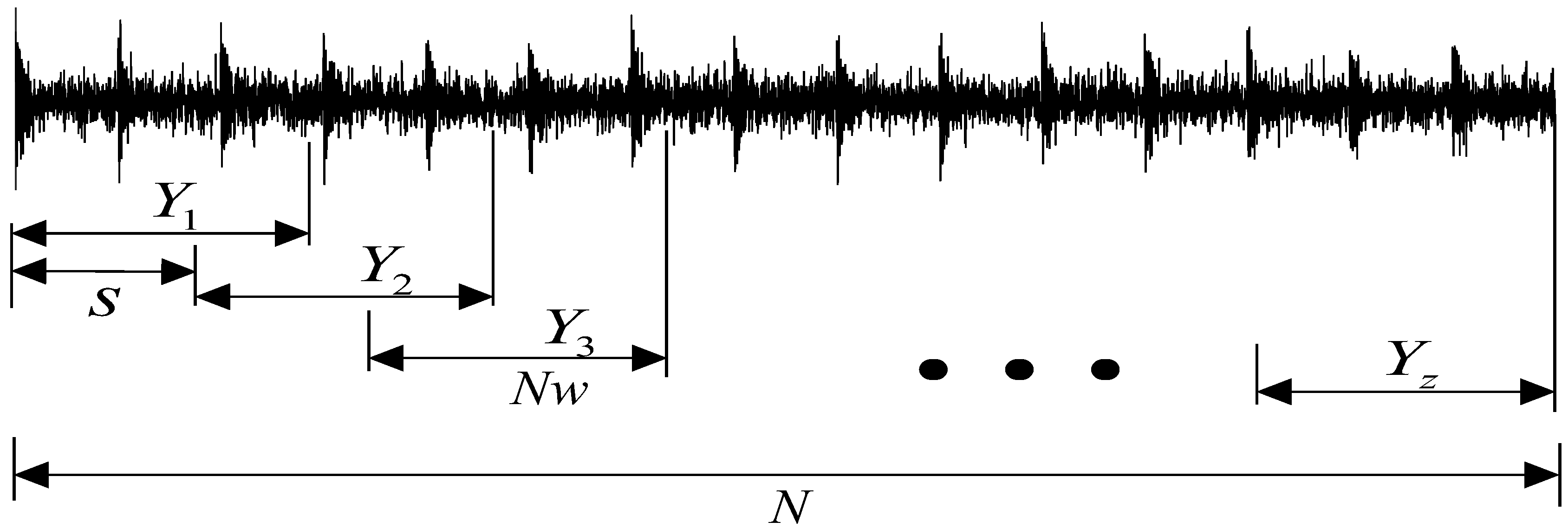
A vibration signal sampled by the sensor from rotating machinery is always a discrete time series with strong background noise. To research more detail of vibration signal, the original time series is separately divided into an array of short sliding signal segments by overlapping rectangle window.
As seen in Figure 2, the sliding coefficient () is employed to an analyzed vibration signal (where ) with the length of . Firstly, the original signal is truncated into each signal segment and the th short sliding signal segment is expressed as follows:
Then the SMS with dimension is provided by the following form:
where is the number of short sliding segment and is the corresponding length.The scope of the sliding coefficient is defined as ;
To further extract the local feature information hidden in the SMS, sparse reconstruction by Hankel-matrix is utilized. Firstly, each column of the SMS is separately transformed into a block Hankel-matrix. Because a multi-dimensional matrix can help to deeply explore and analyze the short sliding signal segment from different perspectives. represents the th block Hankel-matrix of the short time sliding signal and is expressed as
where
Secondly, consider the Hankel-matrix as a graph and calculate the corresponding histogram of matrix data. According to the theory of image processing, the histogram can effectively exhibit the distribution of the pixel intensities in a predefined number of bins which range from the minimum to maximum intensity. On the other side, due to each row of the Hankel matrix being closely correlated, the intensity of data is sparsely distributed in the histogram. In other word, a sparse reconstructed sequence can be effectively achieved from Hankel-matrix by histogram. Then the sparse sequences of the th Hankel-matrix is presented as
And the sparse reconstructed matrix sequence of the SMS can be written as
As mentioned above, employ MDErms to each sparse reconstructed matrix sequence and achieve the corresponding characteristic index. The obtained calculation is called Multiscale Entropy Value Matrix (MEVM):
where
In the matrix, the column of MEVM is called Multiscale Entropy Value Sequences (MEVS) and represents the feature information of the same segment in different scales. And the row of MEVM separately represents the characteristic and complexity of different segments.
According to Section 2.1, the MEVM is fused into a final MFEVS by LPP. The obtained MFEVS can be written as
3.2. Feature Extraction with MFEVS
Local faults in rotating bearings usually generate an array of periodic impulses in vibration signal. Theoretically, the impulses will excite the system resonance in the form of quasi-periodic or periodic damping oscillation waveform. Besides, MDErms shows a remarkable ability in measuring and quantifying the complexity of a time series. Regular and periodic signals are often characterized by a lower entropy value, whereas interference random signals usually correspond to a higher entropy value. Then, it can be concluded that the short sliding signal segment hidden local fault features is relatively less complex and corresponds to a lower entropy value. Hence, the proposed method will divide the original vibration signal into an array of short sliding segments and separately explore the fault signature by calculating the MDErms of each part.
Having in mind the introduction mentioned above, the fusion feature MFEVS can effectively characterize the complexity and irregularity of the corresponding short sliding segments. If the short sliding segment contains the fault impulse or part, the corresponding entropy value will be relatively small. Then, minimum MDErms is achieved as the following equation:
where is the number of the short sliding signal with minimum MDErms.
As mentioned above, the corresponding optimal short sliding signal is reconstructed as follows:
According to the mechanism of damped oscillation, the short sliding reconstructed signal theoretically characterizes an obviously quasi-periodic oscillation waveform. Besides, in the frequency spectrum of the short sliding reconstructed signal, the dominant frequency part can be regarded as the main resonance frequency band of original vibration signal and used as the optimal coefficient of the FIR bandpass filter.
3.3. FIR Bandpass Filter Design
Filter is widely used in signal processing in order to filter out the components which include the transient impulse feature for fault diagnosis [25]. For vibration signals, it is necessary and essential to design a desired filter to extract the transient impulse from strong background noise and other interference signals. Thus, a finite impulse response (FIR) bandpass filter is introduced to the proposed method in the paper. Compared with infinite impulse response (IIR) filter, FIR filters are inherently stable because they don’t need to feedback and recursive [26,27]. The impulse response of the FIR filter is of finite duration. The output sample of that is a weighted sum of the last input samples, where represents the order of the filter.
The FIR filter has many greater abilities compared with IIR filter: (1) FIR filters are non-iterative and don’t require feedback, which make the implementation simpler. (2) FIR filters can utilize the FFT algorithm due to the finite impulse response, which will make the calculation process faster. (3) FIR filters do well in linear phase which is necessary on essential to phase-sensitive applications. (4) FIR filters are intrinsically stable without the application of the largest value in the input.
As stated above, FIR filters have a good character of filtering out the fault feature and information from the original signal occupied by a large amount of background noise. It is stated that the transient impulse involves a quasi-periodic oscillation damping process which is filled with abundant fault features. The oscillation frequency is quite near to the resonance frequency of the rotating bearing. Therefore, the paper develops the proposed method with a FIR bandpass filter in order to separate the transient impulse from low frequency disturbed signal.
In order to further extract the fault signature, the frequency-domain calculation of the reconstructed short segment is applied as follows:
where is the frequency domain series of .
The main difficult in the designing of FIR filter is how to choose the optimal filter parameters: the central frequency and the bandwidth . Based on the short sliding segment with the minimum MDErms in Equation (24), the optimal parameters of FIR bandpass filter are identified by the following equation:
where is the sampling frequency, is the length of the sliding signal segment, and is the calculated frequency resolution. represents the tracking index of the desired short sliding segment to be analyzed and is the corresponding frequency spectrum where the max value can be viewed as the optimal central frequency of the designed filter. Besides, the bandwidth parameter depends on the frequency resolution . Unlike other traditional filters, the proposed method for the design of bandpass filter is based on the analyzed signal itself and without prior information, which can effectively reduce the error and enhance the flexibility.
4. Simulation Study
According to the mechanical dynamic of free vibration model with damping, a simulated signal for feature extraction is conducted to verify the efficacy of the proposed method. The expression of the simulated faulty signal is shown as follows:
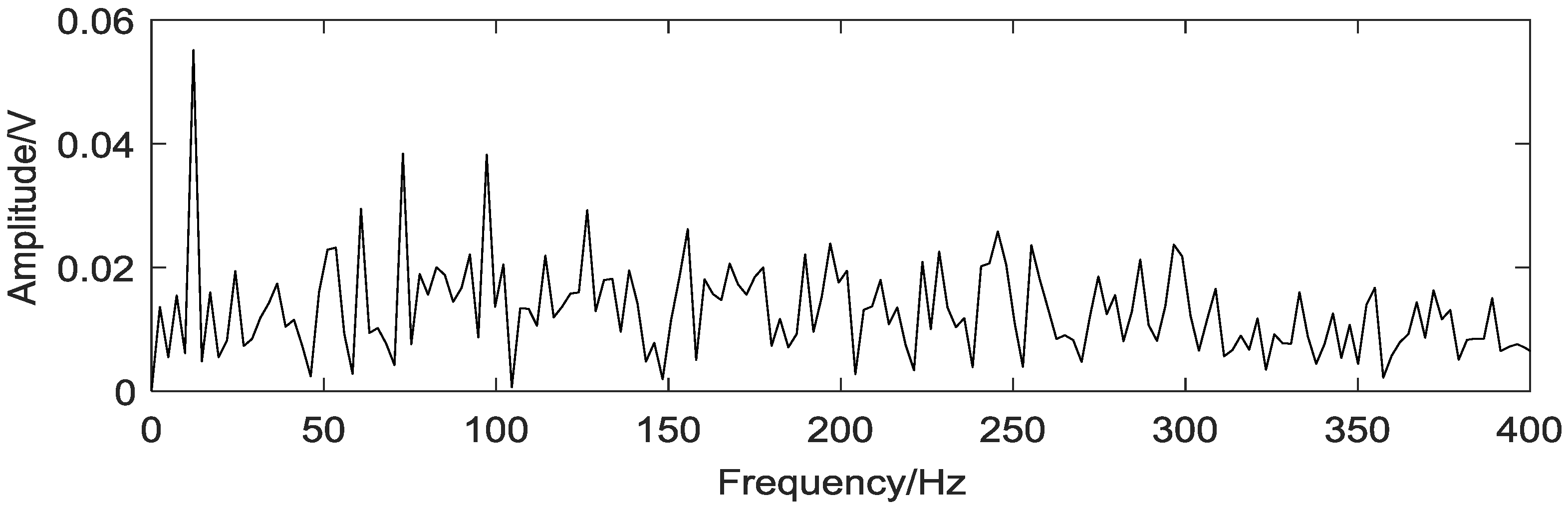
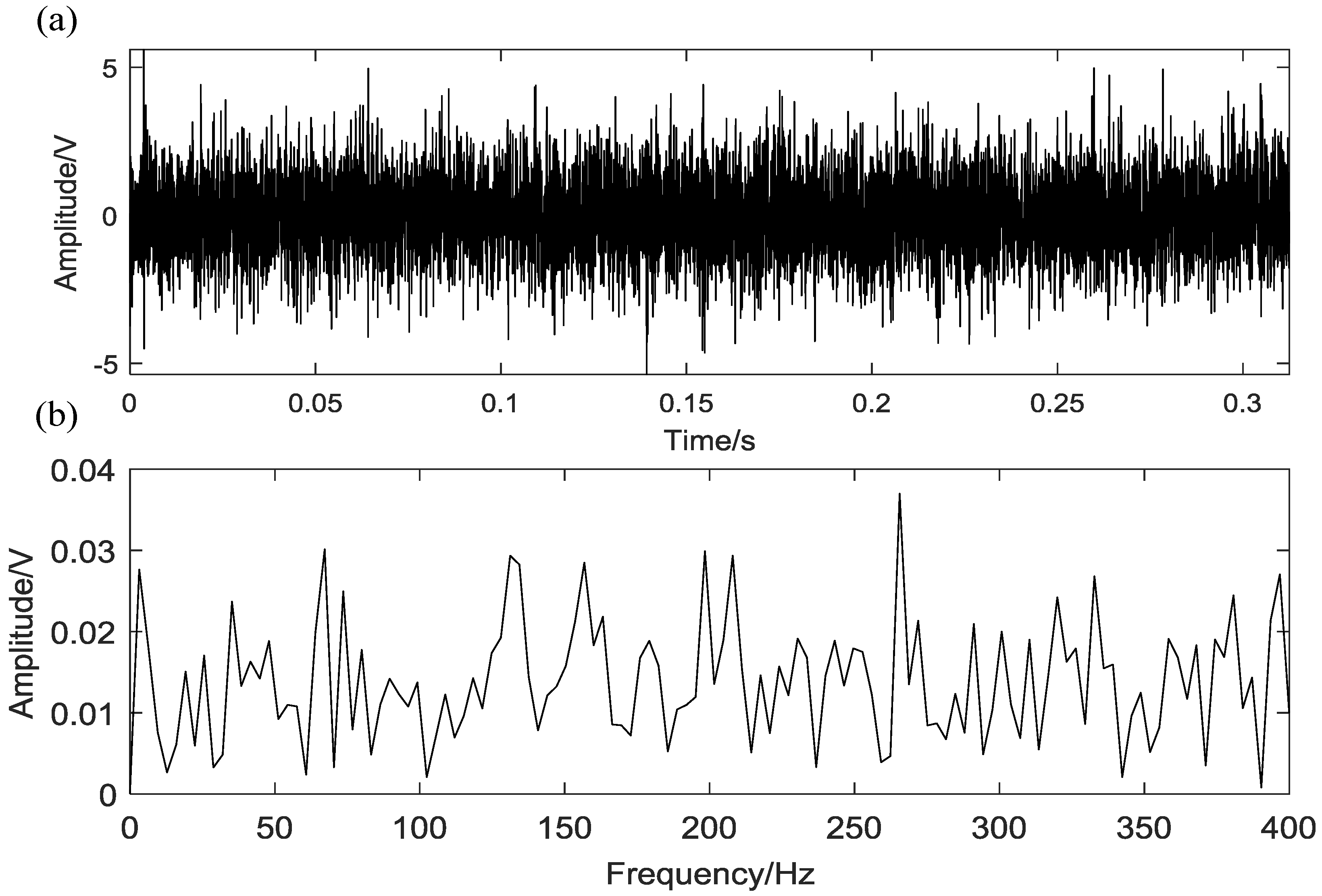
where Hz is the resonance frequency, Hz is the characteristic frequency of the inner-race fault and Hz corresponds to the rotating frequency, and denotes the weak fluctuation of the th impulse. The sampling frequency is 25,600 Hz and the number of data points is 8100. The time domain waveform of the simulated fault signal is illustrated in Figure 3a. Then a gauss white noise is added to the fault signal resulting in the SNR of −8 dB. As seen in Figure 3b, it is difficult to identify the periodic transient impulse from the simulated signal filled with additive noise. The envelope spectrum of the analyzed signal is separately illustrated in Figure 4, where the interference noise makes it hard to recognize the characteristic frequency.
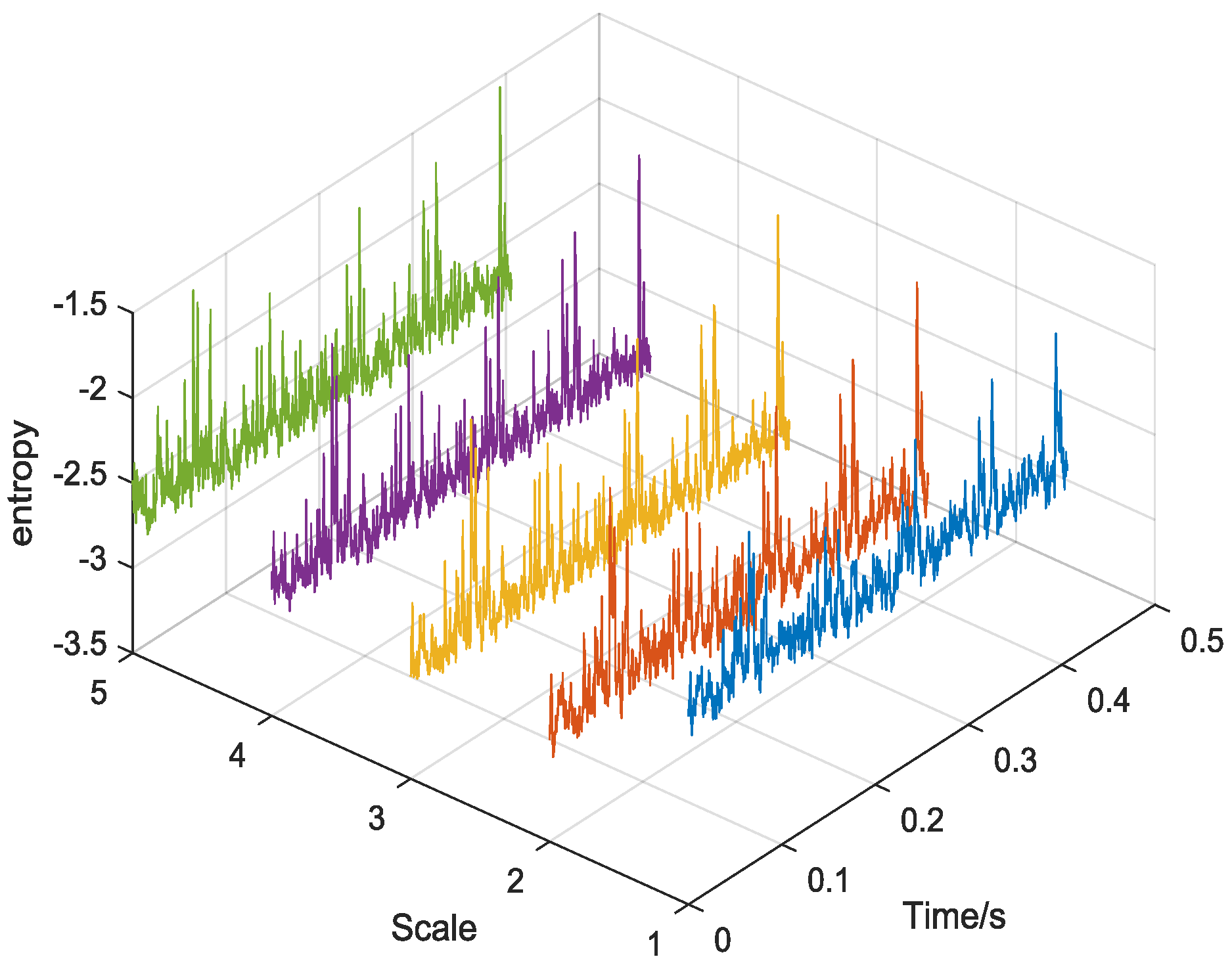
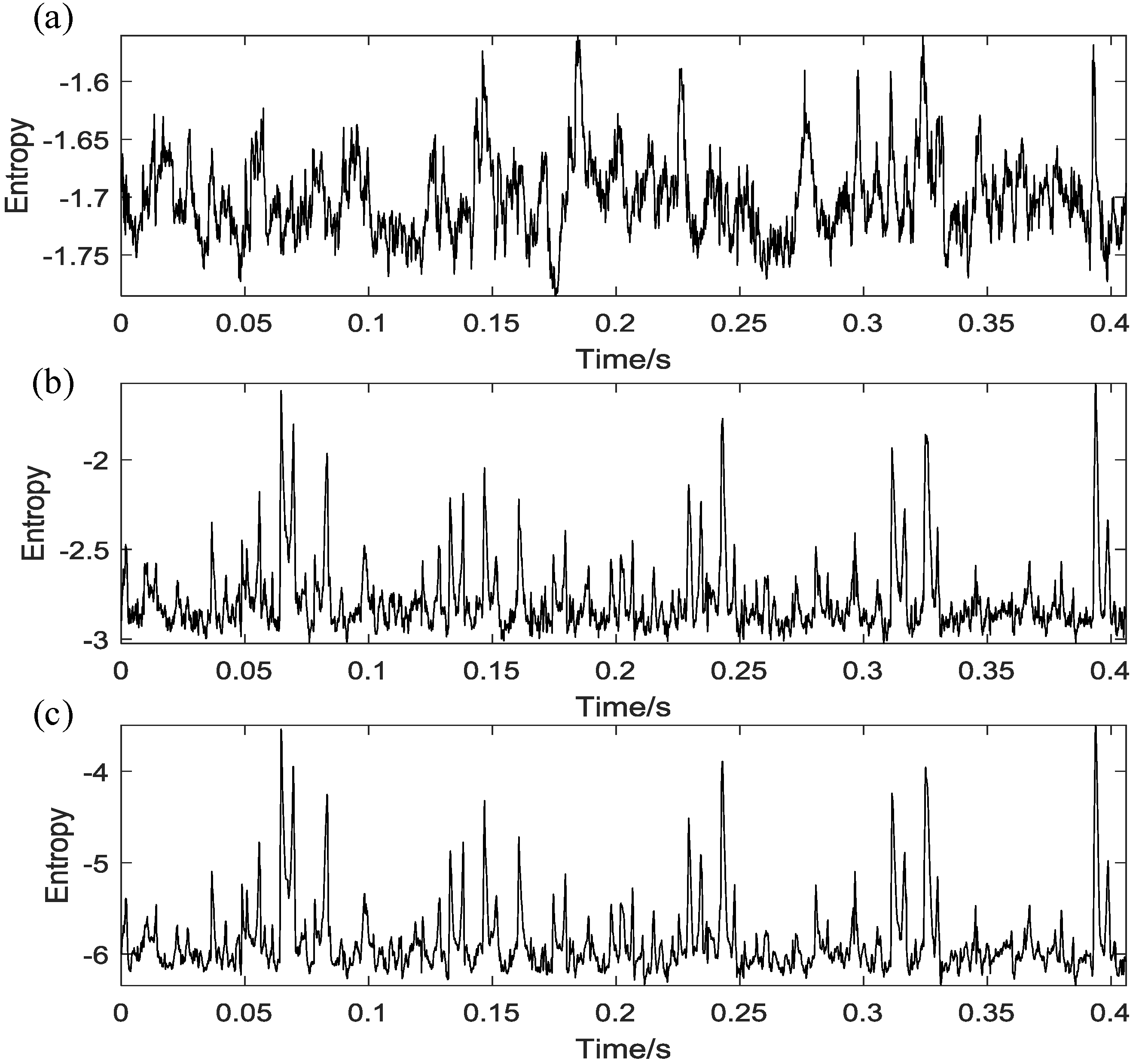
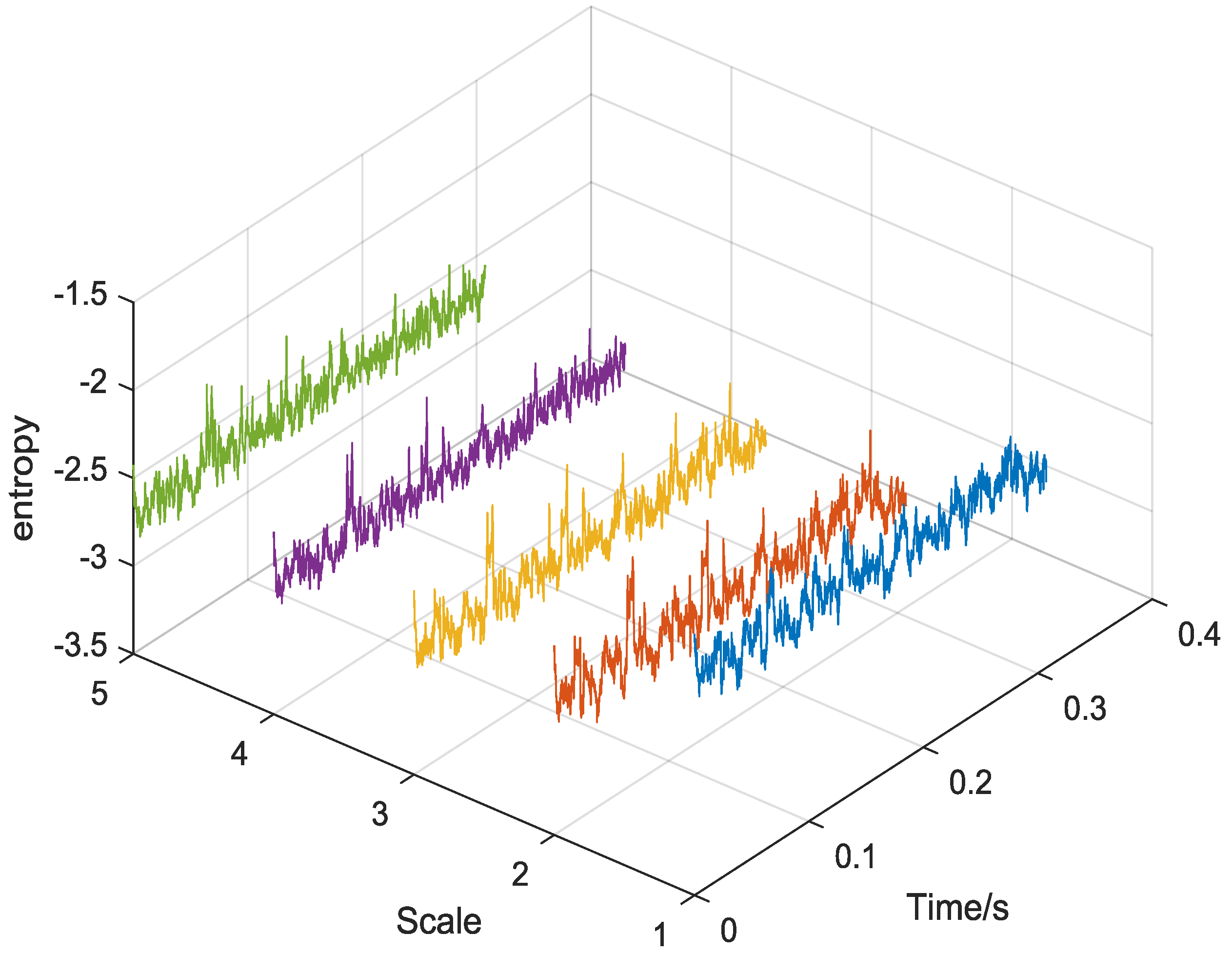
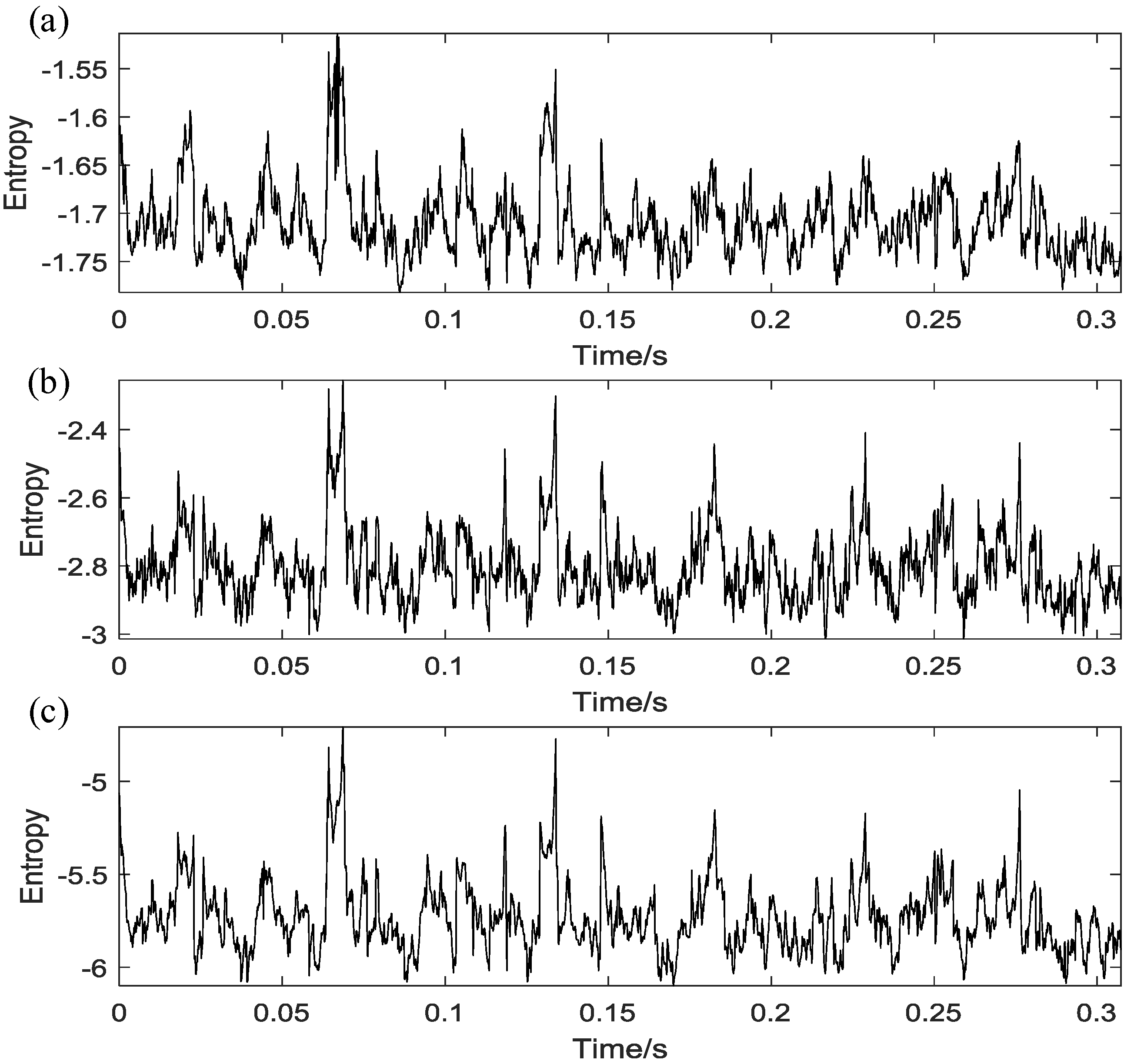
To extract the fault feature efficiently, the proposed method is applied to the simulated noisy signal. The sliding parameter is set to and the analyzed length . As plotted in Figure 5, the entropy value sequences in different scales correspond to the MEVM in Equation (20) separately. To further verify the performance and advantage of the proposed method, a comparison is made as shown in Figure 6. The traditional vector entropy value sequence in Figure 6a fluctuates fairly dramatically, and its amplitude range is too small to distinguish each other. As displayed in Figure 6b, the periodic impulses embedded in the background noise can be effectively identified by the proposed MEVS of 1-scale. Besides, it can be seen in Figure 6c that the final MFEVS combines the characteristic information in different scales and displays rather better stability and performance in comparison with Figure 6a,b.
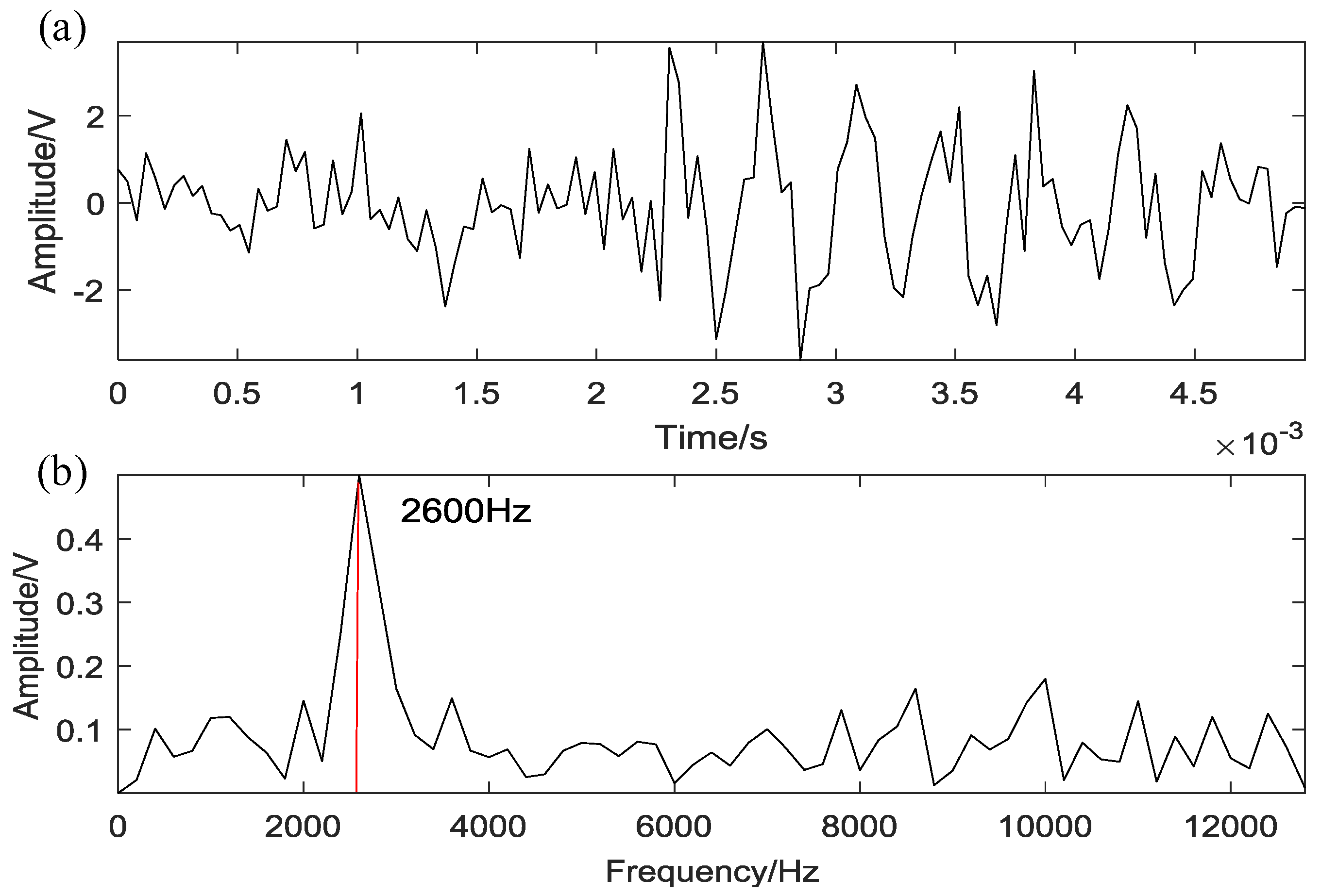
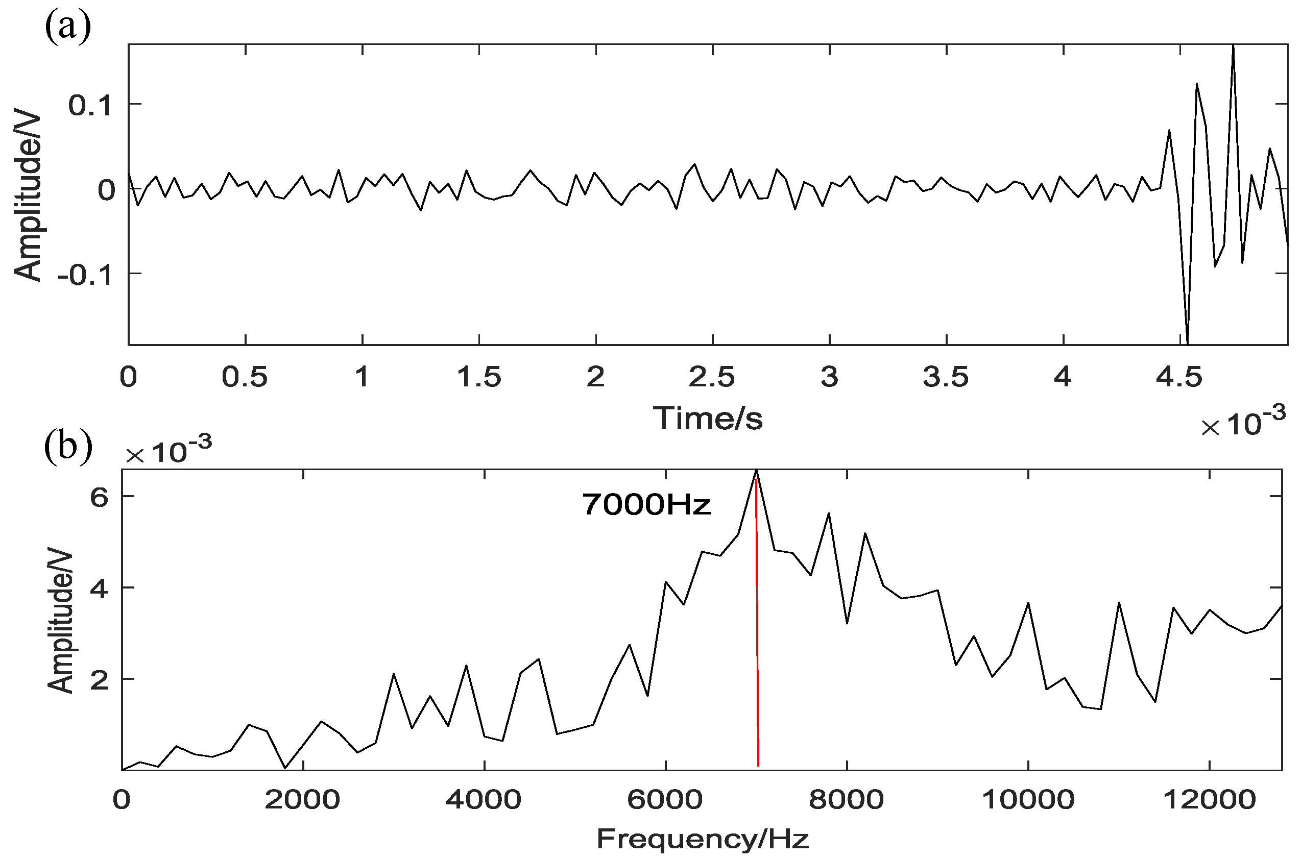
The time-domain waveform of the short sliding segment with minimum MDErms and its frequency spectrum are displayed in Figure 7. Then the corresponding oscillation frequency Hz is obtained, which is same as the predetermined natural frequency value of the simulation signal. Later, the systematic waveform of the filtered faulty signal in time domain is plotted in Figure 8a, where we can find an array of obvious periodic impulses. From the envelope spectrum of the filtered signal in Figure 8b, the main impulses are concentrated at the frequency of and its harmonics, which is exactly equal to the faulty characteristic frequency. Moreover, the envelope waveform in time domain by the FIR filter is shown in Figure 9, where and represent the rotating period and the inner-race failure period separately. It can be seen that the waveform of the proposed MFEVS in Figure 5c and the filtered signal in Figure 9 are quite similar to the original signal in Figure 3a. Therefore, the above simulation demonstrates the effectiveness of the proposed method in bearing fault detection evidently.
5. Experiment Validation
5.1. Test Rig Instruction
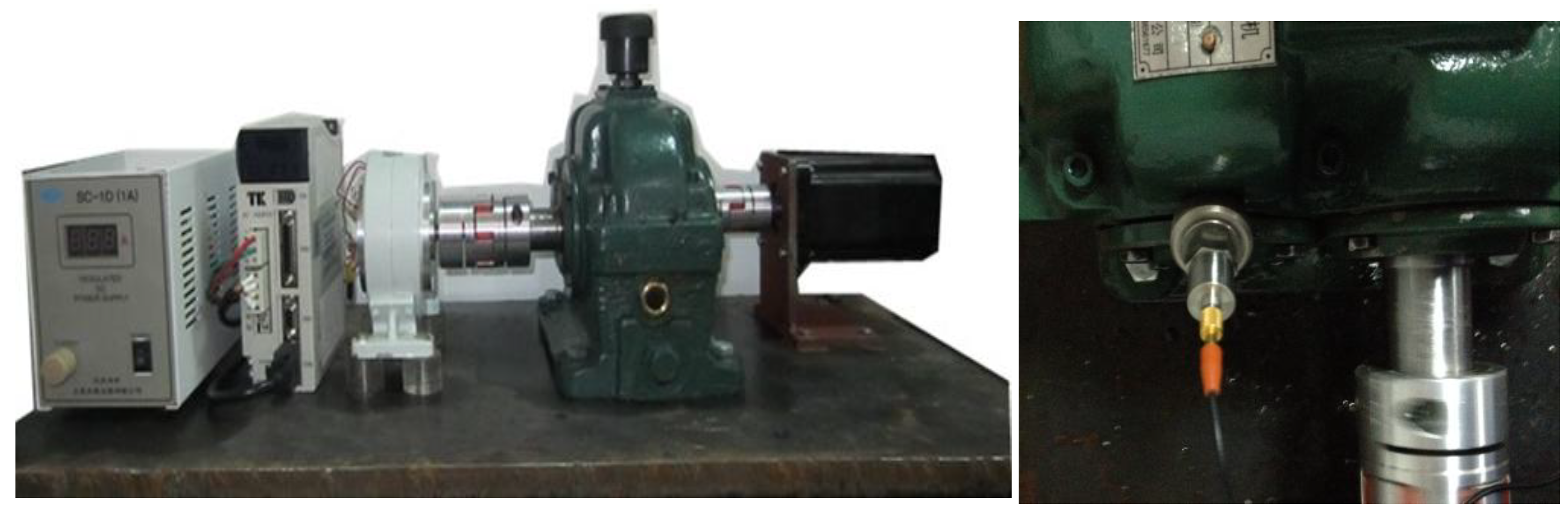
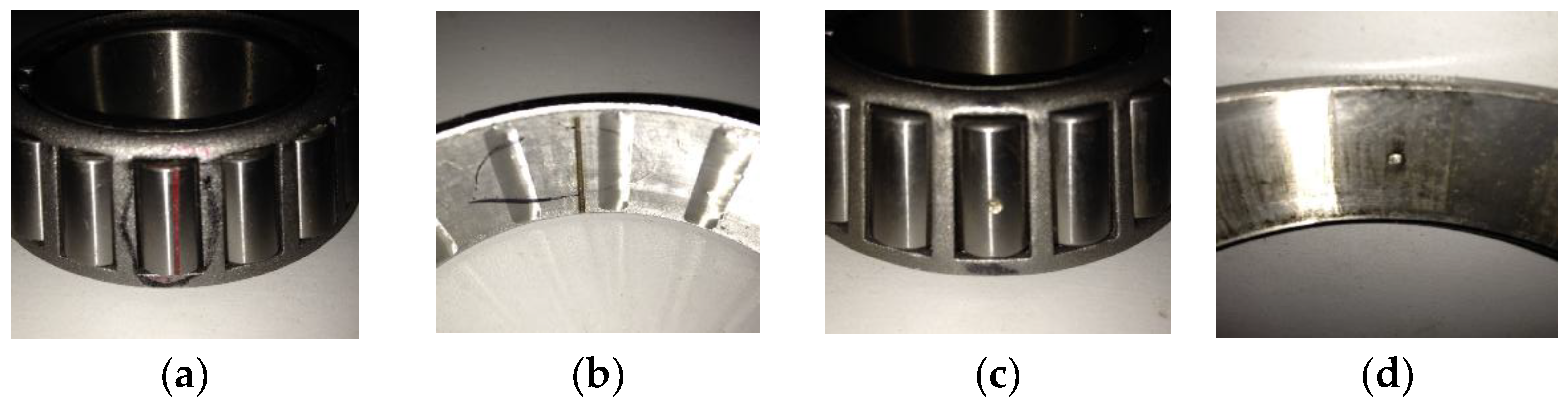
To validate the improvement and effectiveness of the proposed method, an artificial fault experiment of rolling element bearing is performed. As shown in Figure 10, the test rig is composed of three main parts: the electronic control system, data acquisition system, and the drivetrain components including the servo motor and gearbox. The data acquisition system contains a NI 9234 data acquisition card and a Dell laptop with the data acquisition program written by LabVIEW. The vibration signal of the artificial fault bearing was measured by an acceleration sensor with the sampling frequency of 12,800 Hz and the analyzed length of 40,960 points. The bearing types are separately 30,304 and 32,207 tapered roller bearing. As provided in Figure 11, the artificial defects of flaws and single pitting points by electrical discharge matching were separately set on a rolling element and outer raceway.
The theoretical equations are introduced to calculate the defect characteristic frequency of bearings in the experimental process as follows:
where represents the rotating frequency of shaft, denotes the contract angle, and respectively denote the pitch diameter and rolling element diameter of the bearing. Then according to the bearing geometrical parameters displayed in Table 1, the fault characteristic frequency of the rolling element () and outer-raceway () can be separately achieved.
On the other hand, two assessment indicators are introduced for quantifying the performance of the proposed method. The first is the SNR considering the harmonic information about , expressed as follows [28]:
where is the amplitude value of envelope spectrum at frequency . The second is kurtosis, which is commonly used to measure signal impulsiveness in the field of rotating machinery fault diagnosis. Kurtosis is defined as
where represents the average, represents the standard deviation.
5.2. Case 1: Bearing Outer Race Fault
The time-domain waveform and its envelope spectrum of the outer raceway faulty signal with the bearing type of 30,304 are illustrated in Figure 12. As seen in the time-domain waveform, the heavy background noise makes it difficult to identify the fault-related periodic impulses. The envelope spectrum in Figure 12b is unable to extract the defect-related characteristic frequency from the vibration signal under the interference of strong noise. We cannot accurately identify the fault frequency component which is covered with other interference frequency parts including the rotating frequency and low-frequency heavy noise etc. The rotating speed of shaft is 900 Hz and corresponds to a rotating frequency 15 Hz. Then the fault characteristic frequency of outer raceway flaw is calculated to 75.8 Hz.
To improve the accuracy of defect identification and fault diagnosis, the proposed method is applied to the analyzed signal. Table 2 displays the parameters in the method. Firstly, the corresponding entropy value sequences in different scales of the MEVM are illustrated in Figure 13 and all the waveforms show quite similar periodic impulses with time. However, it is still difficult to recognize the fault signature from heavy noise. The waveform of the traditional vector entropy sequence is presented in Figure 14a. As a comparison, the waveform of the proposed MEVS of 1-scale and the final MFEVS are displayed in Figure 14b,c and both have a better remarkable stability than Figure 14a. Moreover, it can be seen that the final MFEVS in Figure 14c presents relatively obvious periodic impulses.
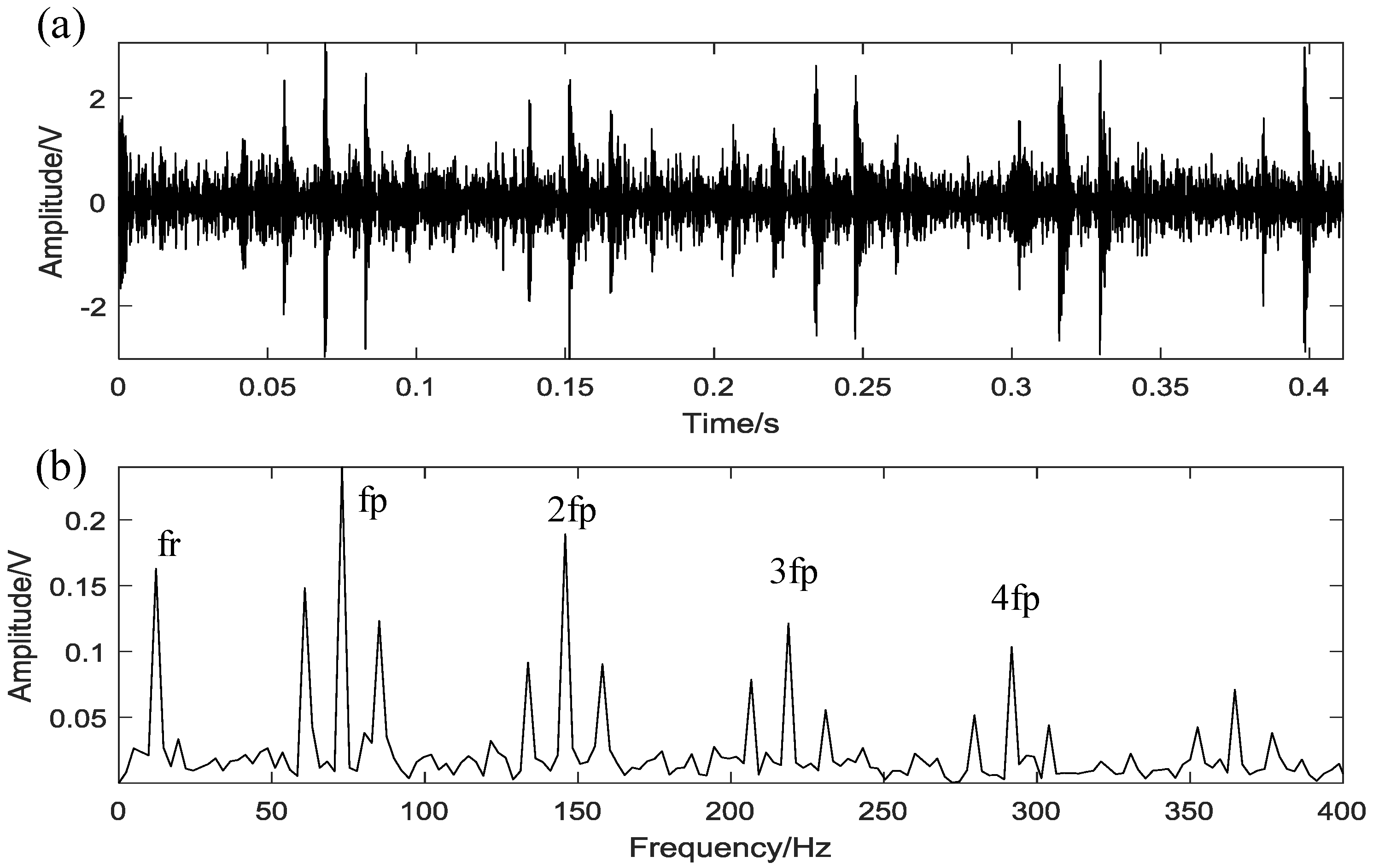
Secondly, the waveform of the optimal short sliding segment with minimum MDErms is illustrated in Figure 15. According to its envelope spectrum in Figure 15b, the resonance frequency 7000 Hz can be identified and then applied to the designed FIR filter. As a result, the time-domain waveform of the filtered signal is plotted in Figure 16a, where the defect-induced impacts appear periodically. From the envelope spectrum of that in Figure 16b, the fault characteristic frequency and its harmonics can be clearly recognized, which is near to the theoretical calculation . Besides, the corresponding envelope waveform of the filtered signal is shown in Figure 17, where and are the rotating period of shaft and the interval period of the outer race fault. Thus, it can be confirmed that the defect should locate in the outer-race of the 30,304 bearing by the proposed method.
To further verify the advantage and superiority of the proposed method in terms of removing irrelevant noise and enhancing fault diagnosis, three traditional feature extraction methods are introduced to make a comparison. The four methods are separately employed to get rid of the heavy noise and extract the defective impulses. As shown in Figure 16, the comparison result visually exposes the disadvantages and limitations of the other three traditional methods. As seen in Figure 16c, the background noise is partly eliminated and some periodic impulses can be observed by the EEMD method. However it is quite hard to find the location of the fault characteristic frequency from the envelope spectrum in Figure 16d. The waveform and envelope spectrum of the WP method is separately plotted in Figure 16e,f, where the defective frequency can’t be recognized. Figure 18 shows the fast kurtogram of outer-race fault signal, and the selected center frequency and bandwidth are 10,666 Hz and 4066 Hz. Then the filtered signal by kurtogram method and the envelope spectrum are separately presented in Figure 16g,h. It can be seen that the kurtogram method doesn’t work well in removing noise and identifying the defective impulses.
Moreover, to visually quantify and assess the performance of different four methods, the two indicators are separately applied to the analyzed result by Equations (30) and (31). As shown in Table 3, the SNR() and kurtosis value of the proposed method are larger than other three traditional methods, indicating that the proposed method is suitable for bearing fault detection. In summary, the comparison result evidently exposes the merit of the proposed method in eliminating background noise and extracting features for the outer race fault vibration signal.
5.3. Case 2: Bearing Rolling Element Fault
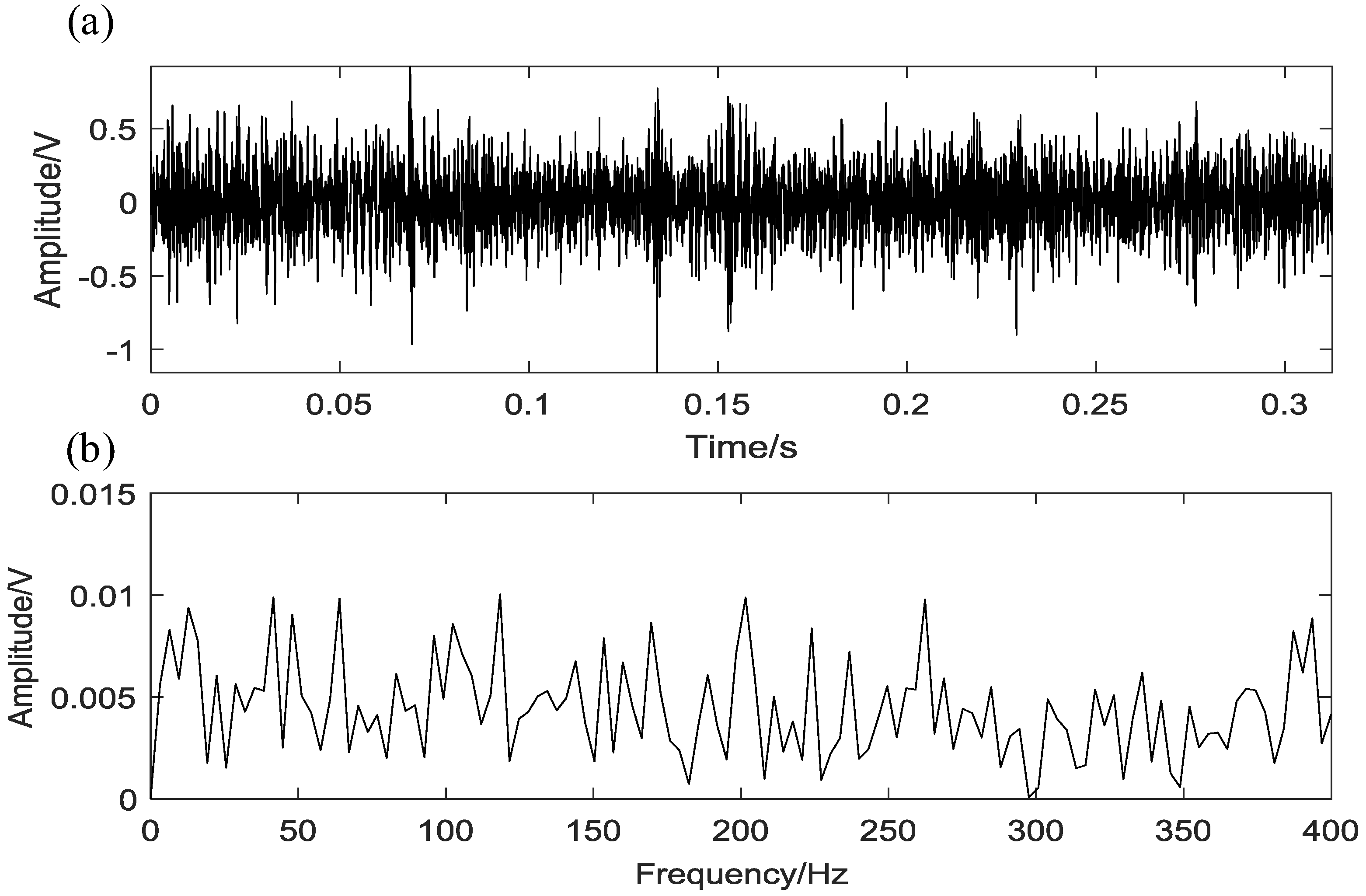
In order to further research the advantage and effectiveness of the proposed method in bearing fault diagnosis, another artificial fault test is operated. As seen in Figure 11a, a groove shape is made on the rolling element of bearing by electrical discharge machining. The defect is in the form of width and depth. When the input shaft is rotating at the speed of , the defective roller passing frequency over the bearing race is calculated to be 62.7 Hz based on Equation (28).
The waveform of the raw roller fault signal in time domain and its envelope spectrum are separately plotted in Figure 19. There is no visible impact in the waveform and the fault signature is submerged in background noise. It can merely figure out the mesh frequency 255 Hz from the envelope spectrum. In the following, the proposed method is also employed to the roller defective vibration signal. Then the entropy value sequences of the MEVM in different scales are illustrated in Figure 20 and the waveforms present visibly similar impulses. Figure 21 is the comparison result of the fault bearing signal by different entropy methods. As seen in Figure 21a, the feature information of the traditional vector entropy sequence without sparse reconstruction is buried by heavy noise. The waveform of the proposed MEVS of 1-scale is displayed in Figure 21b, where some clear periodic impulses can be observed. Besides, the MFEVS in Figure 21c shows a better ability to extract impulse features than Figure 21a,b through visual inspection. Then the optimal short sliding time series with the minimum MDErms is plotted in Figure 22a. According to the envelope spectrum in Figure 22b, the corresponding resonance frequency can be found (3400 Hz) and employed to the designing of FIR bandpass filter. As plotted in Figure 23a, the defective impulses of the filtered signal by the proposed method appear obvious periodically. The fault characteristic frequency and its several harmonics can be observed clearly from the envelope spectrum in Figure 23b, which indicates that the bearing rolling element is broken. Moreover, the corresponding envelope waveform of the filtered signal is displayed in Figure 24, where is the interval period of the roller fault. The waveforms of the MFEVS in Figure 21c and the filtered signal in Figure 24 show visibly similar periodicity, indicating that the proposed MFEVS has good abilities in fault identification and feature extraction.
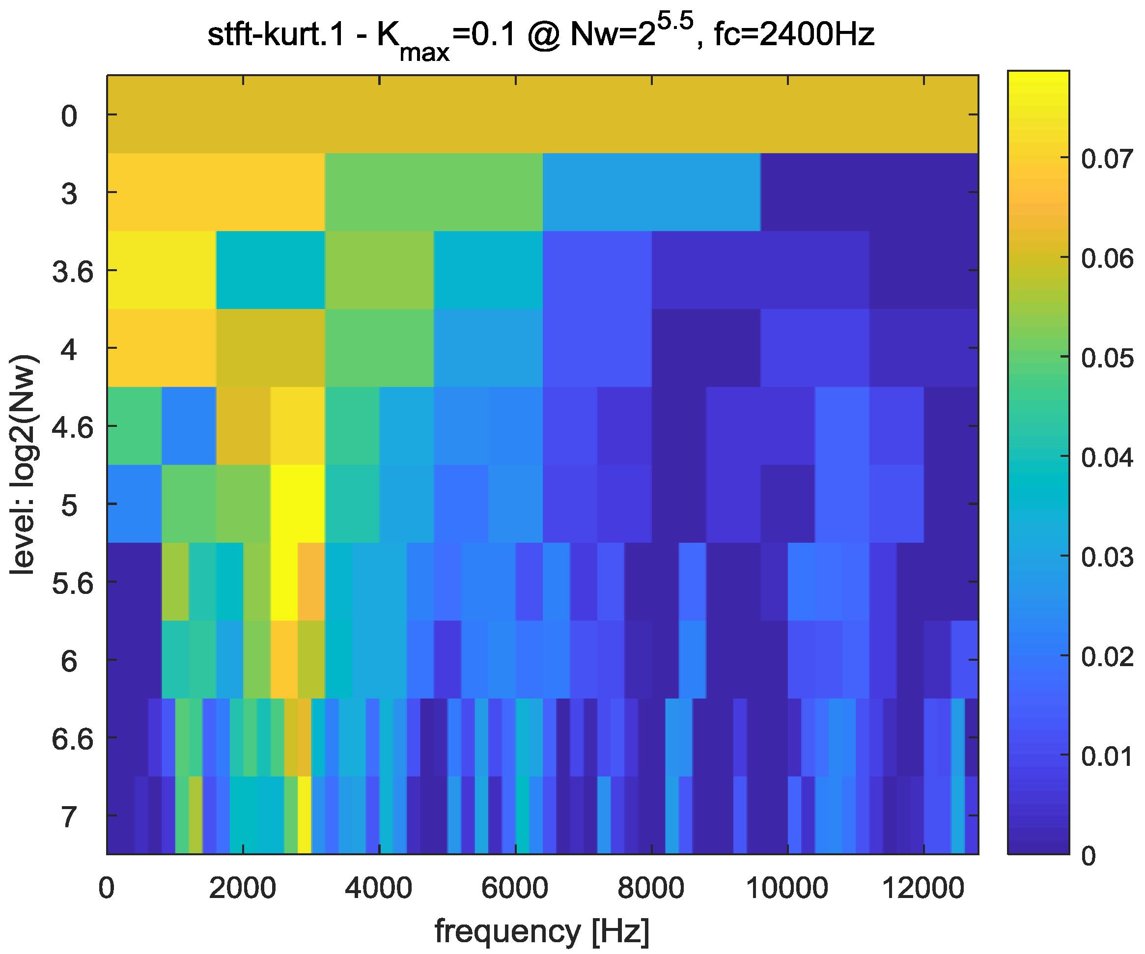
To further extract and analyze the fault information, three different methods are applied to the roller fault signal respectively and the comparison result is shown in Figure 23. As shown in Figure 23c–h, the other three methods all appear to have poor performance and have their own limitations. The waveform of the EEMD method in Figure 23c is full of noise. And several harmonics of the fault characteristic frequency can be roughly identified from the corresponding envelope spectrum. As seen in Figure 23e,f, the WP method just removes some noise segment, and the fault feature is still hard to recognize. The fast kurtogram of roller fault signal in Figure 25 shows that the selected center frequency and bandwidth are 2400 Hz and 64 Hz. Then the signal filtered by the kurtogram and its envelope spectrum are plotted in Figure 23g,h, respectively. It can be concluded that the fast kurtogram method shows a normal performance in eliminating background noise and fault identification.
In the end, the indicators of SNR() and kurtosis are employed to quantify the comparison result. As illustrated in Table 4, the proposed method has the biggest SNR() and kurtosis than other three methods. In summary, through the comparison of the four methods, the proposed method shows great advantage and excellent ability in extracting fault feature information from the roller defective signal.
6. Conclusions
This paper proposes a new feature extraction method for the incipient fault detection of a rolling bearing. Firstly, the SMS truncation and sparse sequences reconstruction by Hankel-matrix are investigated. To effectively address the local feature hidden in sparse sequences, this paper develops the MDErms as a characteristic index, which is suitable for a short time series. Then the MDErms is applied to the sparse sequences to obtain the MEVM. Compared with traditional entropy and MEVM of a single scale, the MFEVS extracted from MEVM has a greater advantage in denoising and extracting local fault feature information. Moreover, a FIR bandpass filter is designed based on the resonance frequency extracted from MFEVS. Simulation studies show that the designed filter is particularly efficient in identifying periodic impulse fault from strong background noise. To further verify the effectiveness and advantage of the proposed method, two different cases of artificial defective bearing experiment are separately performed. In comparison with other traditional methods, the proposed method performs quite excellent in improving the ability of removing noise and identifying weak bearing faults.
Author Contributions
Y.Z. and S.T. conceived the feature extraction method; F.C. designed and performed the experiments; J.X. analyzed and interpreted the results; Y.Z. wrote and drafted the manuscript; all authorship read and approved the final manuscript.
Acknowledgments
The research is supported by the National Natural Science Foundation of China (Grant No.51305392); Zhejiang Provincial Natural Science Foundation of China (Grant No.LZ15E050001, LY17E050009); Youth Funds of the State Key Laboratory of Fluid Power Transmission and Control (SKLoFP_QN_1501); The Fundamental Research Funds for the Central Universities (2018QNA4008).
Conflicts of Interest
The authors declare no conflicts of interest.
References
- Randall, R.B.; Antoni, J. Rolling element bearing diagnostics—A tutorial. Mech. Syst. Signal Process. 2011, 25, 485–520. [Google Scholar]
- He, W.P.; Ding, Y.; Zi, Y.Y.; Selesnick, I.W. Sparsity-based algorithm for detecting faults in rotating machines. Mech. Syst. Signal Process. 2016, 72–73, 46–64. [Google Scholar]
- Dong, G.; Chen, J.; Zhao, F. A frequency-shifted bispectrum for rolling element bearing diagnosis. J. Sound Vib. 2015, 339, 396–418. [Google Scholar]
- Žvokelj, M.; Zupan, S.; Prebil, I. Non-linear multivariate and multiscale monitoring and signal denoising strategy using Kernel Principal Component Analysis combined with Ensemble Empirical Mode Decomposition method. Mech. Syst. Signal Process. 2011, 25, 2631–2653. [Google Scholar]
- Guo, W.; Tse, P.W. A novel signal compression method based on optimal ensemble empirical mode decomposition for bearing vibration signals. J. Sound Vib. 2013, 332, 423–441. [Google Scholar]
- Wang, H.; Gao, J.; Jiang, Z.; Zhang, J. Rotating Machinery Fault Diagnosis Based on EEMD Time-Frequency Energy and SOM Neural Network. Arab. J. Sci. Eng. 2014, 39, 5207–5217. [Google Scholar]
- Wang, J.; He, Q. Wavelet Packet Envelope Manifold for Fault Diagnosis of Rolling Element Bearings. IEEE Trans. Instrum. Meas. 2016, 65, 2515–2526. [Google Scholar]
- Rauber, T.W.; de Assis Boldt, F.; Varejao, F.M. Heterogeneous Feature Models and Feature Selection Applied to Bearing Fault Diagnosis. IEEE Trans. Ind. Electron. 2015, 62, 637–646. [Google Scholar]
- Pincus, S.M. Approximate Entropy as a Measure of System Complexity. Proc. Natl. Acad. Sci. USA 1991, 88, 2297–2301. [Google Scholar] [PubMed]
- Hu, X.; Jiang, J.; Cao, D.; Egardt, B. Battery Health Prognosis for Electric Vehicles Using Sample Entropy and Sparse Bayesian Predictive Modeling. IEEE Trans. Ind. Electron. 2016, 63, 2645–2656. [Google Scholar]
- Costa, M.; Goldberger, A.L.; Peng, C. Multiscale entropy analysis of biological signals. Phys. Rev. E 2005, 71, 21906. [Google Scholar] [CrossRef] [PubMed]
- Humeau-Heurtier, A. The Multiscale Entropy Algorithm and Its Variants: A Review. Entropy 2015, 17, 3110–3123. [Google Scholar] [CrossRef] [Green Version]
- Yan, R.; Liu, Y.; Gao, R.X. Permutation entropy: A nonlinear statistical measure for status characterization of rotary machines. Mech. Syst. Signal Process. 2012, 29, 474–484. [Google Scholar] [CrossRef]
- Li, Y.B.; Xu, M.Q.; Wei, Y.; Huang, W.H. A new rolling bearing fault diagnosis method based on multiscale permutation entropy and improved support vector machine based binary tree. Measurement 2016, 77, 80–94. [Google Scholar] [CrossRef]
- Azami, H.; Rostaghi, M.; Abasolo, D.; Escudero, J. Refined Composite Multiscale Dispersion Entropy and its Application to Biomedical Signals. IEEE Trans. Bio.-Med. Eng. 2017, 64, 2872–2879. [Google Scholar] [CrossRef] [PubMed]
- Rostaghi, M.; Azami, H. Dispersion Entropy: A Measure for Time-Series Analysis. IEEE Signal Proc. Lett. 2016, 23, 610–614. [Google Scholar] [CrossRef]
- Li, M.; Liu, H.; Zhu, W.; Yang, J. Applying Improved Multiscale Fuzzy Entropy for Feature Extraction of MI-EEG. Appl. Sci. 2017, 7, 92. [Google Scholar] [CrossRef]
- Guido, R.C. A tutorial review on entropy-based handcrafted feature extraction for information fusion. Inf. Fusion 2018, 41, 161–175. [Google Scholar] [CrossRef]
- Azami, H.; Rostaghi, M.; Fernandez, A.; Escudero, J. Dispersion entropy for the analysis of resting-state MEG regularity in Alzheimer’s disease. In Proceedings of the 2016 IEEE 38th Annual International Conference of the Engineering in Medicine and Biology Society (EMBC), Orlando, FL, USA, 16–20 August 2016; pp. 6417–6420. [Google Scholar]
- Zhang, H.; Liu, X. Analysis of Parameter Selection for Permutation Entropy in Logistic Chaotic Series. In Proceedings of the 2018 International Conference on Intelligent Transportation, Big Data & Smart City (ICITBS), Xiamen, China, 25–26 January 2018; pp. 398–402. [Google Scholar]
- Ding, X.; He, Q.; Luo, N. A fusion feature and its improvement based on locality preserving projections for rolling element bearing fault classification. J. Sound Vib. 2015, 335, 367–383. [Google Scholar] [CrossRef]
- Ji, Z.; Pang, Y.W.; He, Y.Q.; Zhang, H.F. Semi-supervised LPP algorithms for learning-to-rank-based visual search reranking. Inf. Sci. 2015, 302, 83–93. [Google Scholar] [CrossRef]
- Cong, F.Y.; Zhong, W.; Tong, S.G.; Tang, N.; Chen, J. Research of singular value decomposition based on slip matrix for rolling bearing fault diagnosis. J. Sound Vib. 2015, 344, 447–463. [Google Scholar] [CrossRef]
- Cong, F.; Chen, J.; Dong, G.; Zhao, F. Short-time matrix series based singular value decomposition for rolling bearing fault diagnosis. Mech. Syst. Signal Process. 2013, 34, 218–230. [Google Scholar] [CrossRef]
- Aggarwal, A.; Kumar, M.; Rawat, T.K.; Upadhyay, D.K. Optimal Design of 2D FIR Filters with Quadrantally Symmetric Properties Using Fractional Derivative Constraints. Circ. Syst. Signal Process. 2016, 35, 2213–2257. [Google Scholar] [CrossRef]
- Koshita, S.; Onizawa, N.; Abe, M.; Hanyu, T.; Kawamata, M. Realization of FIR Digital Filters Based on Stochastic/Binary Hybrid Computation. In Proceedings of the 2016 IEEE 46th International Symposium on Multiple-Valued Logic (ISMVL), Sapporo, Japan, 18–20 May 2016; pp. 223–228. [Google Scholar]
- Liu, Y.; Parhi, K.K. Architectures for Recursive Digital Filters Using Stochastic Computing. IEEE Trans. Signal Process. 2016, 64, 3705–3718. [Google Scholar] [CrossRef]
- Zhang, S.B.; Lu, S.L.; He, Q.B.; Kong, F.R. Time-varying singular value decomposition for periodic transient identification in bearing fault diagnosis. J. Sound Vib. 2016, 379, 213–231. [Google Scholar] [CrossRef]
Figure 1.
The diagram of the proposed feature extraction method.
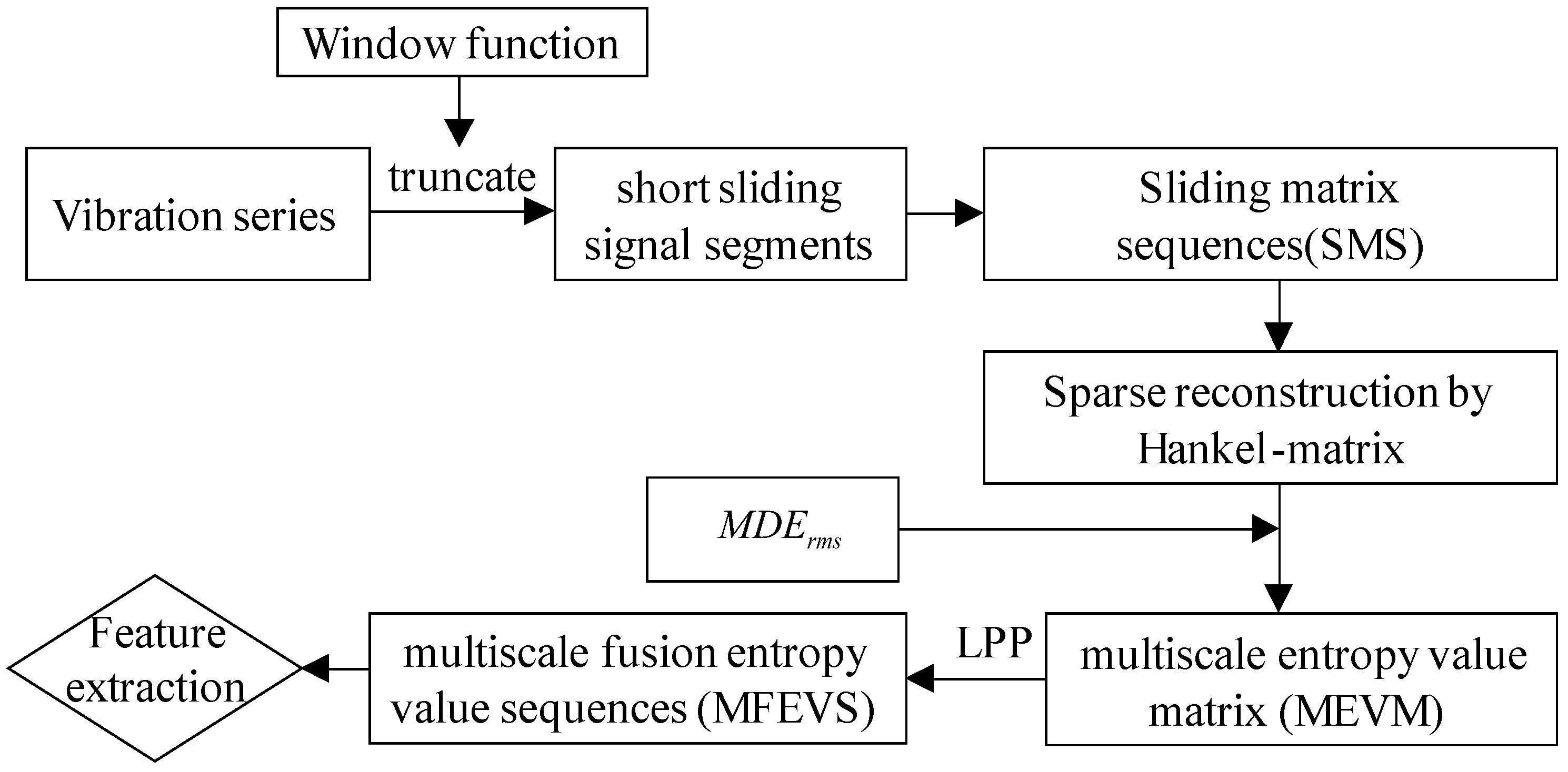
Figure 2.
The diagram of sliding sequence truncation.

Figure 3.
The simulated faulty signal with inner race in time domain: (a) the original signal without noise; (b) the noisy signal with SNR = −8 dB.
Figure 3.
The simulated faulty signal with inner race in time domain: (a) the original signal without noise; (b) the noisy signal with SNR = −8 dB.
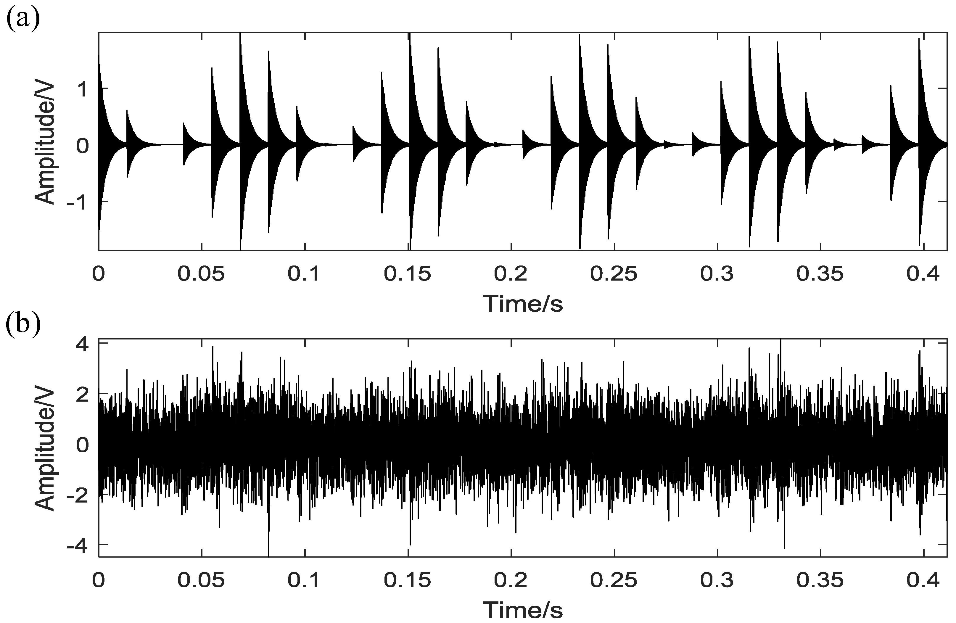
Figure 4.
The envelope spectrum of the noisy signal with SNR = −8 dB.

Figure 5.
Plot of the MEVS for the noisy simulated signal with inner race defect.

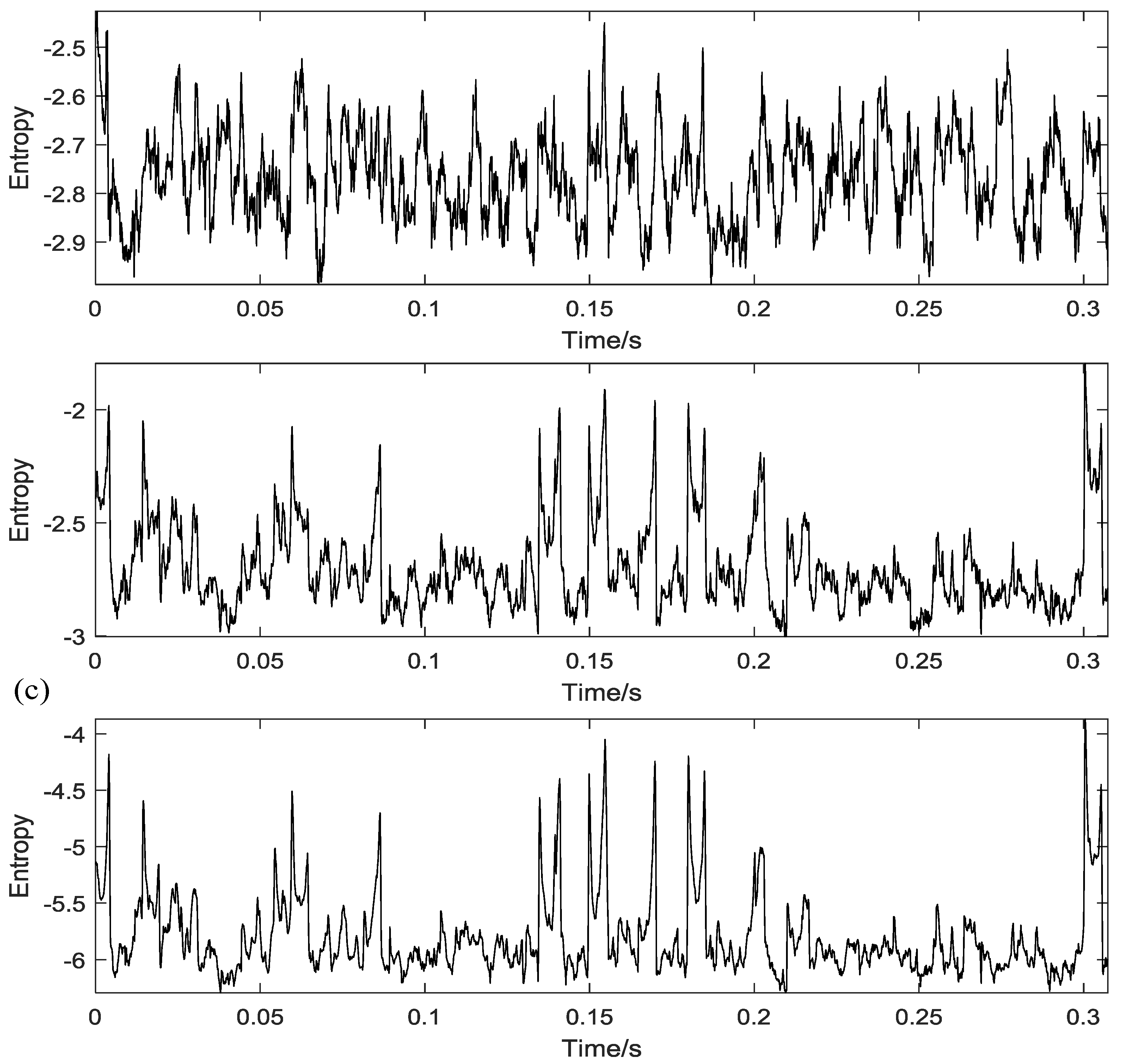
Figure 6.
Comparison results of the noisy simulated signal waveform by different methods: (a) the traditional vector entropy value sequence; (b) the proposed MEVS of 1-scale; (c) The proposed MFEVS.
Figure 6.
Comparison results of the noisy simulated signal waveform by different methods: (a) the traditional vector entropy value sequence; (b) the proposed MEVS of 1-scale; (c) The proposed MFEVS.

Figure 7.
(a) The waveform of the reconstructed short sliding signal; (b) the corresponding frequency spectrum.
Figure 7.
(a) The waveform of the reconstructed short sliding signal; (b) the corresponding frequency spectrum.

Figure 8.
The filtered result of the simulated fault signal by the proposed method: (a) the time domain waveform; (b) the corresponding envelope spectrum.
Figure 8.
The filtered result of the simulated fault signal by the proposed method: (a) the time domain waveform; (b) the corresponding envelope spectrum.

Figure 9.
The envelope waveform of the filtered signal in time domain.
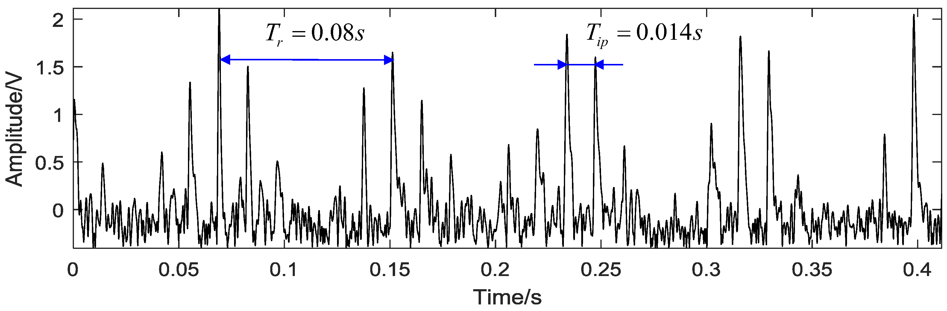
Figure 10.
Test rig.

Figure 11.
The fault types of rolling bearing: (a,c) rolling element defect; (b,d) outer race defect.
Figure 11.
The fault types of rolling bearing: (a,c) rolling element defect; (b,d) outer race defect.

Figure 12.
The signal with outer-race defect: (a) the waveform in time domain; (b) the envelope spectrum.
Figure 12.
The signal with outer-race defect: (a) the waveform in time domain; (b) the envelope spectrum.

Figure 13.
Plot of the Multiscale Entropy Value Sequences (MEVS) for the bearing signal with outer race fault.
Figure 13.
Plot of the Multiscale Entropy Value Sequences (MEVS) for the bearing signal with outer race fault.

Figure 14.
Comparison results of the outer-race fault signal by different methods: (a) the traditional vector entropy value sequence; (b) the proposed MEVS of 1-scale; (c) The proposed Multiscale Fusion Entropy Value Sequence (MFEVS).
Figure 14.
Comparison results of the outer-race fault signal by different methods: (a) the traditional vector entropy value sequence; (b) the proposed MEVS of 1-scale; (c) The proposed Multiscale Fusion Entropy Value Sequence (MFEVS).

Figure 15.
(a) The waveform of the reconstructed optimal short time sliding signal, (b) the corresponding frequency spectrum.
Figure 15.
(a) The waveform of the reconstructed optimal short time sliding signal, (b) the corresponding frequency spectrum.

Figure 16.
The comparison results of the outer-race fault signal by different methods: (a,b) the proposed method; (c,d) the Essential Empirical Mode Decomposition (EEMD) method; (e,f) the Wavelength Packet (WP) method; (g,h) the filter method by fast kurtogram.
Figure 16.
The comparison results of the outer-race fault signal by different methods: (a,b) the proposed method; (c,d) the Essential Empirical Mode Decomposition (EEMD) method; (e,f) the Wavelength Packet (WP) method; (g,h) the filter method by fast kurtogram.
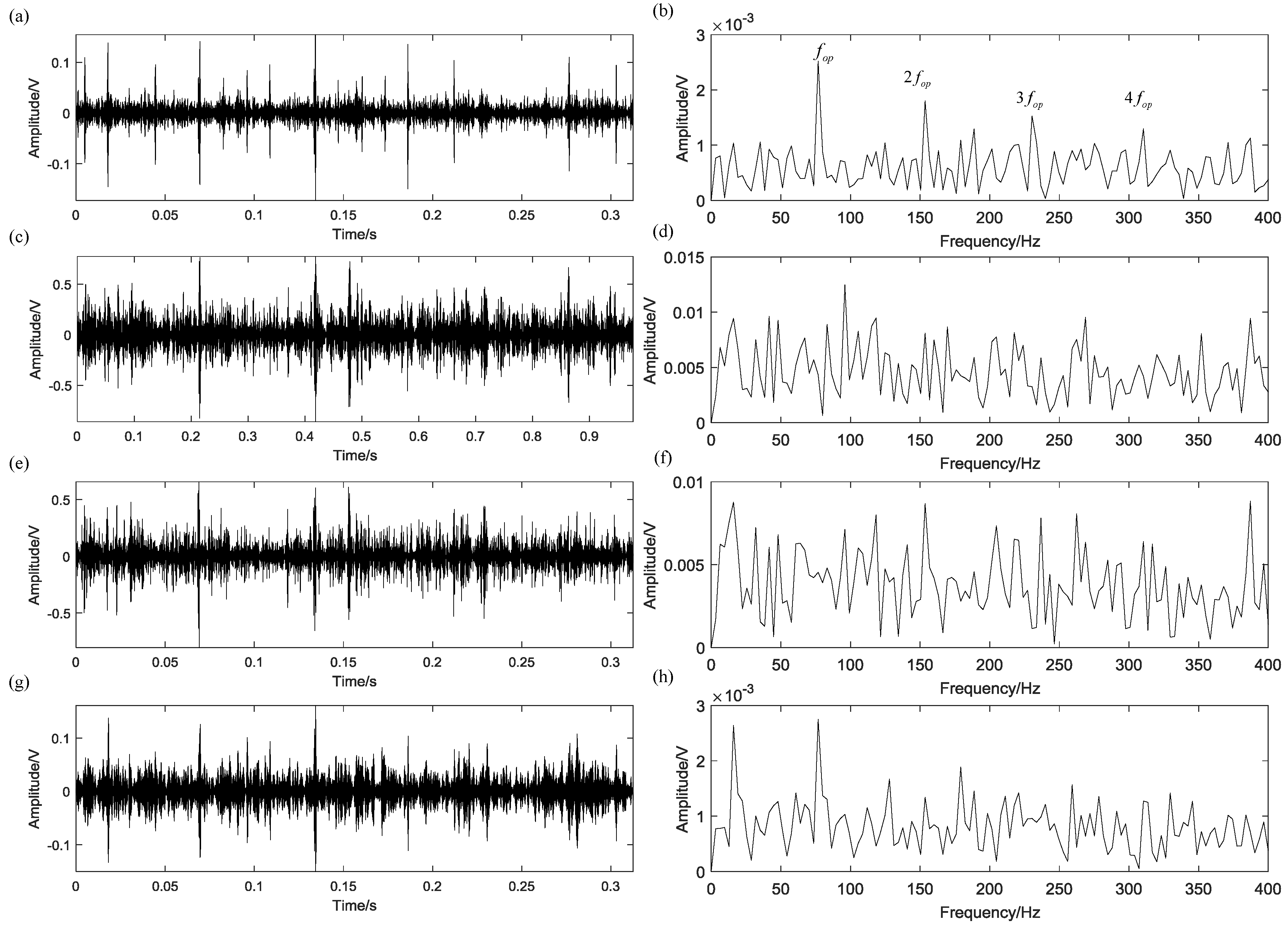
Figure 17.
The envelope waveform of the filtered signal in time domain.
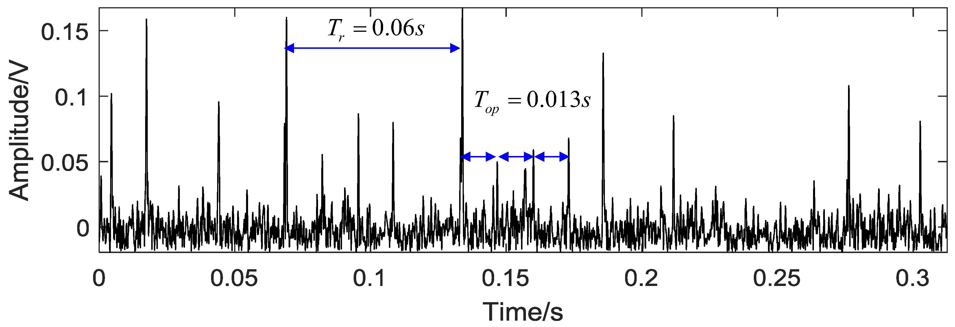
Figure 18.
The fast kurtogram of outer-race fault signal.
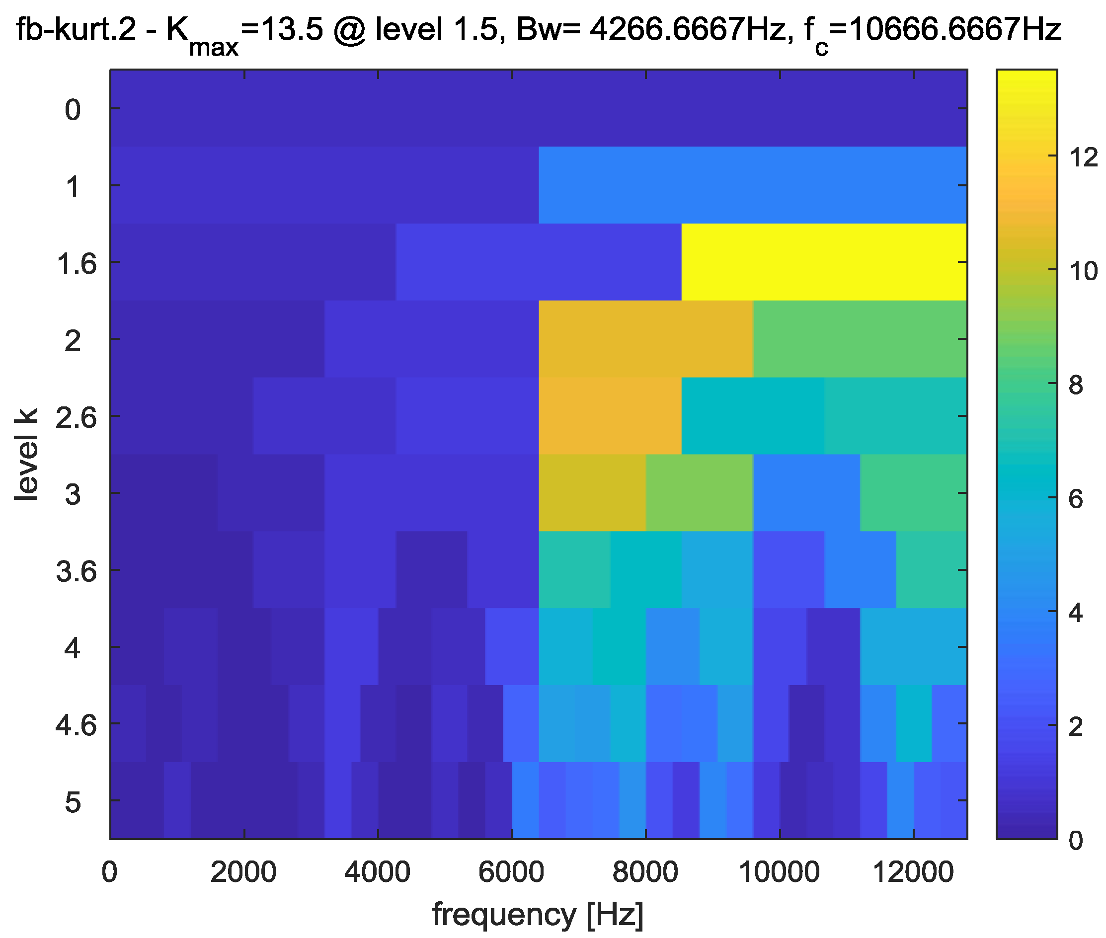
Figure 19.
The bearing signal with roller defect: (a) the waveform in the time domain; (b) the envelope spectrum.
Figure 19.
The bearing signal with roller defect: (a) the waveform in the time domain; (b) the envelope spectrum.

Figure 20.
Plot of the MEVS for the bearing signal with rolling element defect.
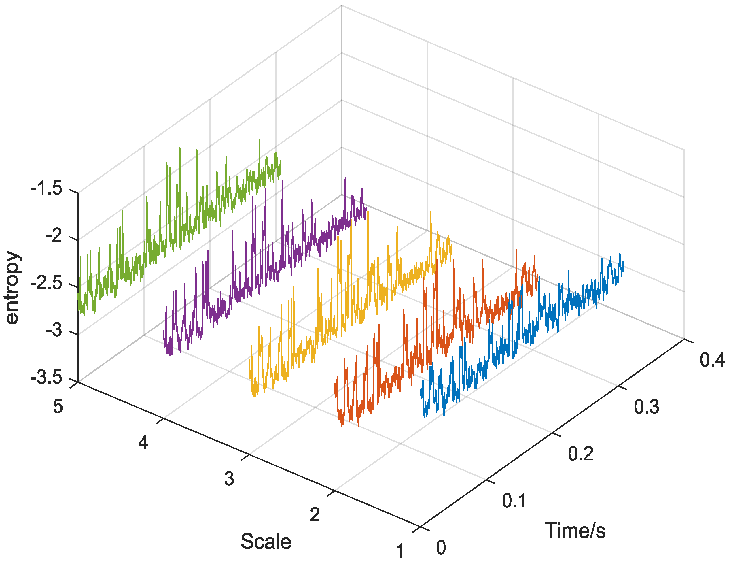
Figure 21.
The comparison results of the roller fault signal by different methods: (a) the traditional vector entropy value sequence; (b) the proposed MEVS of 1-scale; (c) The proposed MFEVS.
Figure 21.
The comparison results of the roller fault signal by different methods: (a) the traditional vector entropy value sequence; (b) the proposed MEVS of 1-scale; (c) The proposed MFEVS.

Figure 22.
(a) The waveform of the reconstructed optimal short time sliding signal; (b) the corresponding frequency spectrum.
Figure 22.
(a) The waveform of the reconstructed optimal short time sliding signal; (b) the corresponding frequency spectrum.
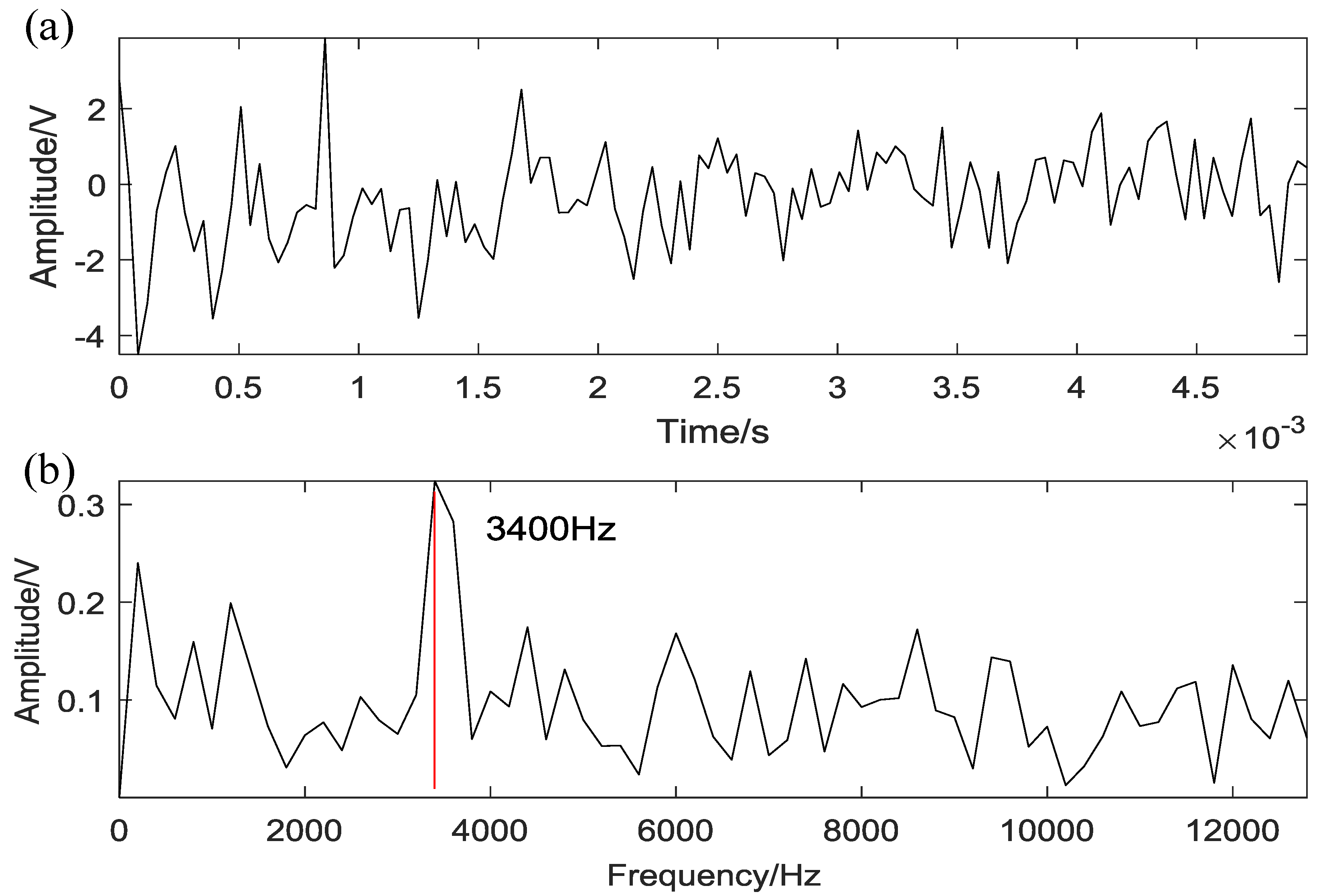
Figure 23.
The comparison results of the roller fault signal by different methods: (a,b) the proposed method; (c,d) the EEMD method; (e,f) the WP method; (g,h) the filter method by fast kurtogram.
Figure 23.
The comparison results of the roller fault signal by different methods: (a,b) the proposed method; (c,d) the EEMD method; (e,f) the WP method; (g,h) the filter method by fast kurtogram.
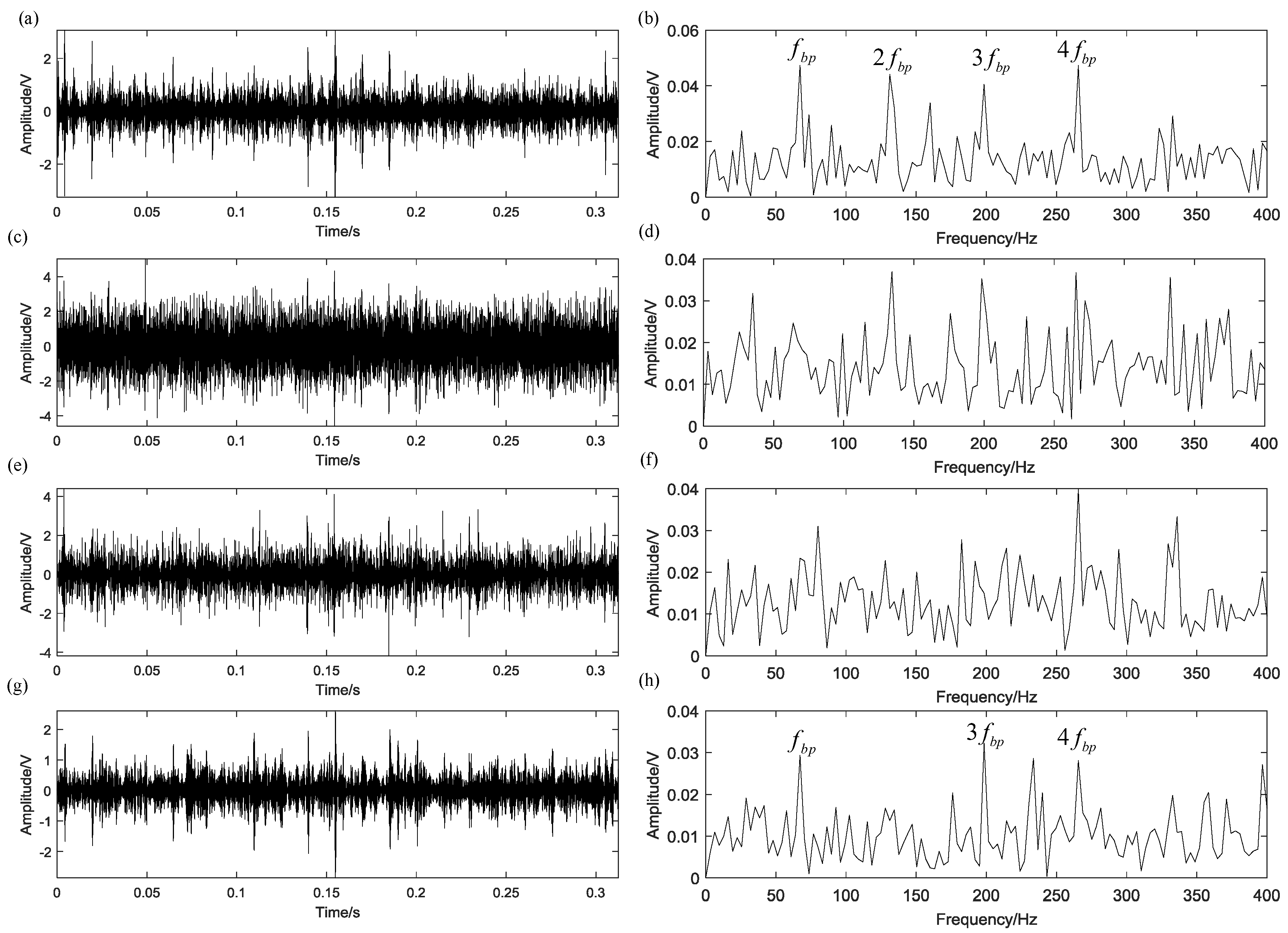
Figure 24.
The envelope waveform of the filtered signal in time domain.
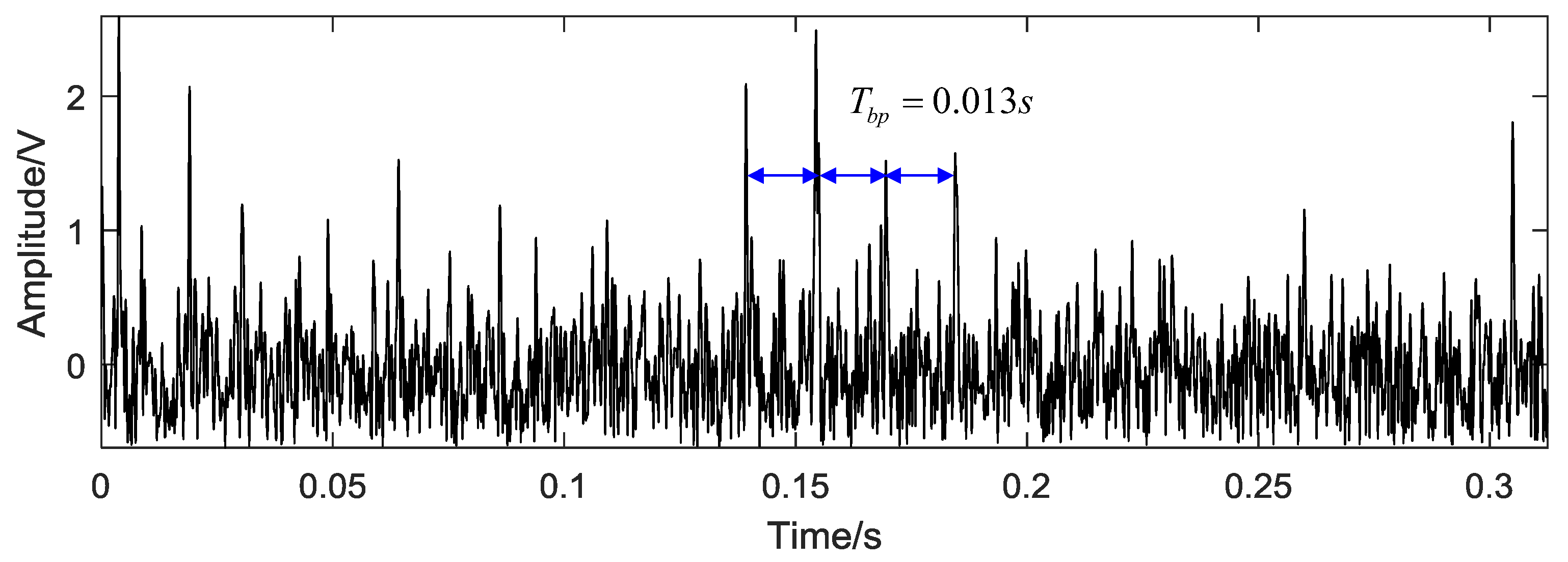
Figure 25.
The fast kurtogram of the rolling element fault signal.

Table 1.
Structure parameters of rolling element bearings.
| Type | Pitch Diameter/D (mm) | Ball Diameter/d (mm) | Number of Roller (Z) | Contact Angle/ |
|---|---|---|---|---|
| 32,207 | 53.31 | 9.52 | 17 | 14.04 |
| 30,304 | 36.35 | 8.26 | 13 | 11.3 |
Table 2.
The parameter in the proposed method.
| Type | |||||
|---|---|---|---|---|---|
| value | 6 | 2 | 6 | 1 | 128 |
Table 3.
The comparison results of the outer-race fault signal by different methods.
| Raw Signal | Proposed Method | EEMD | WP | Fast Kurtogram | |
|---|---|---|---|---|---|
| SNR ()/dB | −24.1 | −15.9 | −21.3 | −22.5 | −17.4 |
| Kurtosis | 3.54 | 14.1 | 4.7 | 4.1 | 4.8 |
Table 4.
The comparison results of the rolling element fault signal by different methods.
| Raw Signal | Proposed Method | EEMD | WP | Fast Kurtogram | |
|---|---|---|---|---|---|
| SNR()/dB | −25.7 | −15.4 | −22.6 | −19.6 | −17.7 |
| Kurtosis | 3.1 | 4.5 | 3.3 | 4.1 | 3.4 |
© 2018 by the authors. Licensee MDPI, Basel, Switzerland. This article is an open access article distributed under the terms and conditions of the Creative Commons Attribution (CC BY) license (http://creativecommons.org/licenses/by/4.0/).
Share and Cite
MDPI and ACS Style
Zhang, Y.; Tong, S.; Cong, F.; Xu, J. Research of Feature Extraction Method Based on Sparse Reconstruction and Multiscale Dispersion Entropy. Appl. Sci. 2018, 8, 888. https://doi.org/10.3390/app8060888
AMA Style
Zhang Y, Tong S, Cong F, Xu J. Research of Feature Extraction Method Based on Sparse Reconstruction and Multiscale Dispersion Entropy. Applied Sciences. 2018; 8(6):888. https://doi.org/10.3390/app8060888
Chicago/Turabian StyleZhang, Yidong, Shuiguang Tong, Feiyun Cong, and Jian Xu. 2018. "Research of Feature Extraction Method Based on Sparse Reconstruction and Multiscale Dispersion Entropy" Applied Sciences 8, no. 6: 888. https://doi.org/10.3390/app8060888
Note that from the first issue of 2016, this journal uses article numbers instead of page numbers. See further details here.