Analytical Calculation of Photovoltaic Systems Maximum Power Point (MPP) Based on the Operation Point


1
Instituto Universitario de Microgravedad “Ignacio Da Riva” (IDR/UPM), Universidad Politécnica de Madrid, ETSI Aeronáutica y del Espacio, Plaza del Cardenal Cisneros 3, 28040 Madrid, Spain
2
Departamento de Sistemas Aeroespaciales, Transporte Aéreo y Aeropuertos (SATAA), Universidad Politécnica de Madrid, ETSI Aeronáutica y del Espacio, Plaza del Cardenal Cisneros 3, 28040 Madrid, Spain
*
Author to whom correspondence should be addressed.
Appl. Sci. 2017, 7(9), 870; https://doi.org/10.3390/app7090870
Submission received: 24 July 2017
/
Revised: 14 August 2017
/
Accepted: 18 August 2017
/
Published: 25 August 2017
(This article belongs to the Section Energy Science and Technology)
Abstract
:This work proposes a new analytical model to extract the 1-Diode/2-Resistor solar cell/panel equivalent circuit parameters. The methodology is based on a reduced amount of experimentally measured information: short-circuit current, the slope of the I-V curve at that point, the open-circuit voltage, and the current and voltage levels, together with the slope of the I-V curve at the instantaneous operation point. This procedure is specially designed to analyze the performance of autonomous photovoltaic systems, which are most of the primary sources for spacecraft power. Results show good agreement with experimental data. Furthermore, this methodology allows for fast and accurate I-V curve maximum power point (MPP) identification.
1. Introduction
1.1. The Solar Cell/Panel Equivalent Circuit Models
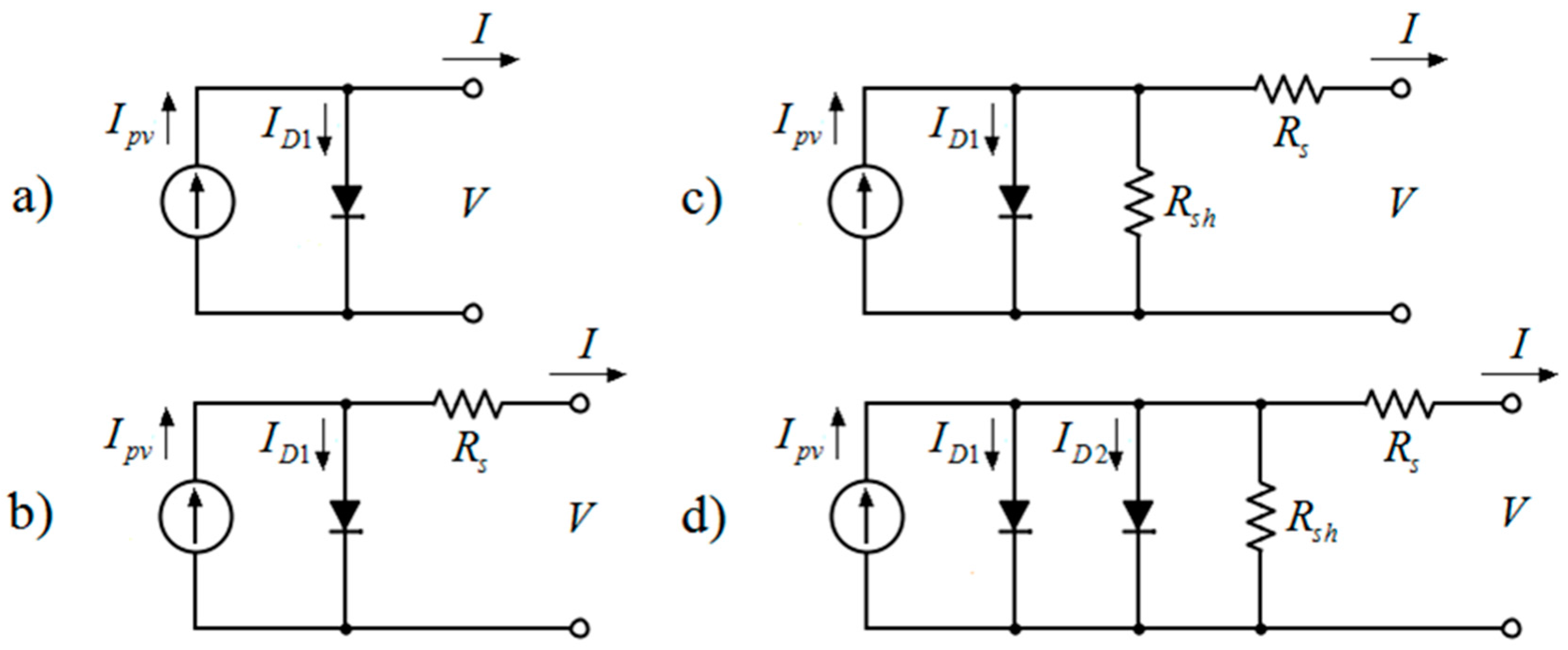
The performance of photovoltaic systems (solar cell/panels), that is, the output current/voltage curve (I-V curve), is usually studied using an equivalent circuit model. This equivalent circuit consists of a current source with one or two diodes connected in parallel, and up to two resistors, one connected in parallel and the other one in series, to take into account energy losses in this model. Based on these electronic components, four basic configurations are normally used when studying photovoltaic systems (see Figure 1):
- (1)
- The 1-diode model, whose equation to relate the output current, I, to the output voltage, V, is:where Ipv is the photocurrent delivered by the constant current source, I0 is the reverse saturation current corresponding to the diode, VT is the thermal voltage (VT = kT/q, where k is the Boltzmann constant, T the temperature expressed in kelvin, and q is the electron charge), a is the ideality factor that takes into account the deviation of the diodes from the Shockley diffusion theory, and N is the number of series-connected cells in the photovoltaic system to be analyzed (obviously, N = 1 in case of a single cell).
- (2)
- The 1-diode/1-resistor model, whose main equation is:where Rs is the series resistor.
- (3)
- The 1-diode/2-resistor model, whose main equation is:where Rsh is the shunt resistor.
- (4)
- And finally, the 2-diode/2-resistor model, whose main equation is:
Obviously, the parameters of these equations need to be estimated to adapt the corresponding model to the real performance of the solar cell/panel behavior. This parameter extraction can be carried out based on analytical or computational methods. A quite complete review of the different methods for fitting the equivalent circuit to the solar cell/panel behavior can be found in recent works by Jena and Ramana [1] and Humada et al. [2].
In Figure 2 and Figure 3, the well-known experimental data (i.e., the I-V curve) of a R.T.C. France silicon cell (La Radiotechnique Compelec, Paris, France) and a Photowatt PWP201 solar panel (Photowatt, Bourgoin-Jallieu, France) from the work by Easwarakhanthan et al. [4] is plotted (the data from the work by Easwarakhanthan et al. have been used as reference in a very large number of scientific works related to photovoltaic performance, according to google scholar it has been cited more than 150 times since its publication—20 times in 2017—), together with five curves corresponding to Equations (1)–(4). See in Table 1 the characteristic data from these experimental curves, including the inverse of the slope of the I-V curves at the short-circuit and open-circuit points, respectively Rsh0 and Rs0. The extracted parameters from these equations are included in Table 2 and Table 3. The extraction was carried out analytically, based on procedures already described in previous works [3,5,6,7], using different conditions to extract the parameters in each case:
- 1-diode model (indicated as 1D in Figure 2 and Figure 3, and Table 2 and Table 3): the three characteristic points from the testing data (short circuit current, Isc, open circuit voltage, Voc, and current and voltage levels at maximum power point, Imp, Vmp), are used as the three conditions needed to extract the values of parameters Ipv, I0 and a in Equation (1). The I-V curve resulting from this model crosses the aforementioned maximum power point, but it is not assured that this condition is reached at this point.
- 1-diode/2-resistor model, two procedures are used in this case:
- (a)
- Four conditions procedure (indicated as 1D/2R-1 in Figure 2 and Figure 3, and Table 2 and Table 3): the three characteristic points and the slope of the I-V curve at maximum power point, together with a pre-established value of the ideality factor (reasonably, in the bracket from a = 1.1 to a = 1.3 [8]), are used as the four conditions needed to extract the values of parameters Ipv, I0, Rs and Rsh in Equation (3).
- (b)
- Five boundary conditions procedure (indicated as 1D/2R-2 in Figure 2 and Figure 3, and Table 2 and Table 3): the three characteristic points, the slope of the I-V curve at maximum power point, and the inverse of the slope of the I-V curve at the short-circuit point, Rsh0, are used as the five conditions needed to extract the values of parameters Ipv, I0, a, Rs and Rsh in Equation (3).
- 2-diode/2-resistor model (indicated as 2D/2R in Figure 2 and Figure 3, and Table 2 and Table 3): the three characteristic points, the slope of the I-V curve at maximum power point, and the inverse of the slope of the I-V curve at the short-circuit and open-circuit points, Rsh0 and Rs0, together with the pre-established value of the ideality factor corresponding to the second diode (a2 = 2.0), are used as the four conditions needed to extract the values of parameters Ipv, I01, I02, a1, Rs and Rsh in Equation (4).
As mentioned, the parameters extracted are included in Table 2 and Table 3. They can be compared with the ones from other authors that used Easwarakhantahan et al. experimental data [4] to describe their solar cell/panel equivalent circuit parameter extraction procedures. The accuracy of each curve, defined by the comparison with the testing result, ∆I = Iexp − I, is shown in the bottom graph of Figure 2 and Figure 3. Besides, in order to compare the five equivalent circuits, a normalized root mean square error (RMSE) has been also included in Table 2 and Table 3:
This comparison parameter is based on the RMSE proposed by Askarzadeh and Rezazadeh [9,10]. The use of the normalized root mean square error allows the comparison between results from different photovoltaic technologies and configurations. From the figures and the tables, it can be observed that the more complicated the model is, the best results are obtained in terms of accuracy. However, it should be pointed out that the 2-diode/2-resistor model fitted to the Photowatt PWP201 solar panel shows a negative value of one of the diode reverse saturation currents. This result indicates that the model does not reflect the physical properties of the solar panel, although mathematically it fits the testing results very well.
1.2. The Problem of Determining the I-V Curve Maximum Power Point (MPP)
We can conclude from the above results that analytical methods need the characteristic points of the I-V curve in order to extract the parameters of a photovoltaic system (cell or panel) equivalent circuit. The advantage of using these points lies in the small amount of information needed, which is normally provided by the manufacturer. However, if experimental data are the source to calculate the equivalent circuit of a solar cell/panel using an analytical method, the main problem turns to be the accurate determination of the I-V curve’s maximum power point (MPP). Unlike the other two characteristic points (short-circuit and open-circuit), whose determination is relatively simple, the MPP correct estimation requires multiple measurements at different voltage levels around this particular point. This fact weakens one of the main advantages of the analytical methods, as quite large resources are required to determine the MPP accurately. This is, in fact, one of the most relevant problems in the solar energy industry: how to make the photovoltaic devices work at the maximum extractable power despite the changing conditions (temperature, solar radiation, loads…). Different maximum power point tracking (MPPT) techniques have been developed in the past decades to track continuously the maximum power point and force the photovoltaic device to work as close as possible.
Among the MPPT methods described in the available literature (see a quite complete review of the MPPT methods in the recent works by Lyden and Haque [11], Koutroulis et al. [12], Verma et al. [13], and Liu et al. [14]), it is possible to distinguish between offline and online methods [15]. In offline methods, the maximum power point is calculated using information regarding the panel I-V curve. One of the main advantages of these methods is the possibility to change the operating voltage instantaneously in order to reach the voltage level corresponding to the maximum output power. The problem lays in the reduced accuracy obtained when calculating that voltage level, due to the complexity of the equations used for estimating the equivalent circuit parameters. Additionally, another problem shown by the offline methods is the absence of feedback to know whether the prediction is correct.
On the other hand, feedback is available in online methods (e.g., perturb and observe methods). As a consequence, using these methods the maximum power point (MPP) of the I-V curve is continuously searched for, and the operating voltage accordingly corrected. However, online methods also have some drawbacks, as large periods can be required to estimate the MPP voltage level.
Finally, there are also hybrid solutions, such as combining two different methods, each one from one of the aforementioned categories. The offline method is used to get a quick approximation of the MPP, whereas the online method is used to improve the result.
1.3. Methodology Proposed to Calculate the Maximum Power Point (MPP)
In the present work, an alternative analytical method is proposed to extract the 1-diode/2-resistor equivalent circuit parameters from a reduced number of experimental measurements. Bearing in mind that measuring both short-circuit and open-circuit points are also simple operations, the main problem remains the maximum power point (MPP) determination, as the operating voltage of this point is, in principle, unknown. In the proposed methodology, equations corresponding to the maximum power point and its derivative are replaced by their equivalents at any other point (Ii, Vi).
This procedure is similar to other parameter-extraction methods that do not require the MPP, and use another point of the I-V curve instead. For example, Laudani et al. [16] developed a non-direct iterative method that avoids using the MPP. The works by other authors such as Garrigós et al. [17], Toledo et al. [18], Blanes et al. [19] should be also mentioned, as they fit the equivalent circuit model to the I-V curve with a limited number of points.
Once the equivalent circuit parameters have been extracted, the proposed analytical method can be used to predict the MPP location on the I-V curve. Furthermore, the use of the proposed analytical method for maximum peak power tracking (MPPT) is analyzed, as proposed by some of the aforementioned authors [17,18,19]. The proposed calculation procedure can be briefly summarized as follows:
- Obtain the short circuit current, Isc, and the inverse of the I-V curve’s slope at that point, Rsh0, of the solar cell/panel as in MPPT offline methods (short circuiting the panel or with pilot cells).
- Obtain the open circuit voltage, Voc, of the solar cell/panel like in MPPT offline methods (opening the circuit or with pilot cells).
- Monitor the solar panel to obtain the instantaneous working point, that is, the operation point (Ii, Vi) and dI/dV|i.
- Extract the 1-diode/2-resistor equivalent circuit model parameters.
- Calculate the maximum power point Imp, Vmp.
As mentioned, this methodology has advantages in both offline and online methods. On the one hand, in the case of the offline methods the method allows for the instantaneous calculation of the desired value of the operating voltage, but with higher precision. On the other hand, in the online methods, there is feedback that improves the accuracy in each step, because the operating point is used to recalculate the maximum power point, which increases the accuracy of the calculation as the operating point approaches to the maximum power point.
The use of the characteristic points (short circuit and open voltage) can be a problem if they are measured during the solar panel operation, as it could represent “an unacceptable power loss” [19]. Nevertheless, on the one hand, this power loss will depend on the data acquisition frequency; on the other hand, pilot cells could overcome this drawback, as mentioned above.
The present work is the last contribution from the IDR/UPM Institute within the research framework on space solar panel performance analysis. This project has proven to be successful from both the scientific and academic points of view (the results from the research on solar panels, once obtained, are immediately used by the students of the Master in Space Systems (MUSE), organized by the IDR/UPM Institute [20,21,22]). It should be pointed out that one of the aims of the work carried out at the IDR/UPM is to obtain procedures that obtain the quickest results in relation to foreseeing the behavior of the photovoltaic systems (within a reasonable accuracy level), as in autonomous systems such as the space systems, the fastest solutions are normally preferred. The results obtained with the aforementioned analytical methods, together with some mathematical approaches [23], have been used for the solar power supply estimations related to UPMSat-2 [24] and Lian-Hé/UNION missions. It is also fair to mention that the key factor in large photovoltaic power stations (solar parks) is different. In these industrial power plants, the power estimations should always provide the most accurate results, as the impact of this accuracy on the economic revenue can be huge [25], and the calculation resources and time consumptions being proportionally large as well.
This work is organized as follows. The methodology developed is explained in Section 2, whereas the results, firstly applied to both the photovoltaic cell and panel mentioned in this section (R.T.C. France and Photowatt PWP201, respectively), and then applied to a SELEX 5-cell space photovoltaic module (the solar panels of the UPMSat-2 satellite integrate several of these modules, both series and parallel connected), are included in Section 3. Finally, conclusions are summarized in Section 4.
2. Equations Proposed to Calculate the 1-Diode/2-Resistor Equivalent Circuit and the Maximum Power Point (MPP)
Particularizing the 1-diode/2-resistor circuit equation in the characteristic points of the I-V curve, the following equations can be obtained [3]:
where Equation (6) corresponds to the short-circuit point, Equation (7) to the slope at the short circuit point, Equation (8) to the open-circuit point, Equation (9) to the maximum power point, and finally, Equation (10) is derived from the condition dP/dV = 0 at that point.
The alternative proposed in this work is to substitute the Equations (9) and (10) with their equivalents at any point (Ii, Vi):
From Equations (6)–(8), (11) and (12) the following explicit and decoupled equations can be deduced for parameters Ipv, I0, Rsh, a and Rs:
where:
Once the parameters of the solar cell/panel equivalent circuit have been extracted, it is possible to calculate the maximum power voltage, Vmp, and maximum power current, Imp, by solving Equations (9) and (10). These two equations can be reduced to a two-equation system with one implicit equation only:
where:
3. Results. Maximum Power Point (MPP) Determination
In this section, the accuracy of the proposed method for calculate the maximum power point is analyzed.
3.1. R.T.C. France Solar Cell and Photowatt PWP201 Solar Panel
In the first place, the data from the R.T.C. France solar cell and the Photowatt PWP201 solar panel are used. Two points of the I-V curve, with their corresponding slope (one at each side of the MPP), were selected for both photovoltaic devices:
- R.T.C. France solar cell. Point 1: (Vi, Ii) = (0.4137, 0.728), and Point 2: (Vi, Ii) = (0.4784, 0.632).
- Photowatt PWP201 solar panel. Point 1: (Vi, Ii) = (11.8018, 0.963), and Point 2: (Vi, Ii) = (13.1231, 0.8725).
The results from the parameter extraction are included in Table 4 and Table 5, together with results from other authors’ works (the results can also be compared to the ones included in Table 2 and Table 3). From these results, it can be assumed that the proposed method presents similar (but slightly larger) values of the normalized root mean square error, ξ, when compared to other methods that use the MPP instead of an operation point that replaces it. Besides, it also seems that the accuracy is higher if the voltage of operation point is larger than the voltage at MPP. Finally, it should also be highlighted that the accuracy depends on the determination of the slope of the I-V curve at the short-circuit point, which is quite challenging in this case due to the lack of points within this area in both I-V curves from the aforementioned work of Easwarakhanthan et al.
With regard to the maximum power point (MPP) estimated from the equivalent circuit based on the calculated parameters, the results are the following:
- R.T.C. France solar cell (Point 1): (Vmp, Imp) = (0.4529, 0.6874), which implies a 0.197% error with regard to the maximum power supplied (Table 1).
- R.T.C. France solar cell (Point 2): (Vmp, Imp) = (0.4497, 0.6932), which implies a 0.329% error with regard to the maximum power supplied (Table 1).
- Photowatt PWP201 solar panel (Point 1): (Vmp, Imp) = (12.5249, 0.9212), which implies a 0.018% error with regard to the maximum power supplied (Table 1).
- Photowatt PWP201 solar panel (Point 2): (Vmp, Imp) = (12.6174, 0.9157), which implies a 0.155% error with regard to the maximum power supplied (Table 1).
3.2. SELEX Galileo 5-Cell Photovoltaic Assembly
Once the proposed method has been checked with the well-known testing results by Easwarakahnthan et al. [4], new and more recent experimental data, i.e., the I-V curve, from a SELEX Galileo 5-cell Photovoltaic Assembly tests have been also used to validate the procedure (see Figure 4 and Figure 5). These testing results were measured at CIEMAT (CIEMAT –Centro de Investigaciones Energéticas, Medioambientales y Tecnológicas– is the Spanish national center for energy and environmental research, and it is the reference laboratory related to solar panel qualification in Spain. It involves the highest qualified personnel and facilities in relation to photovoltaic testing [33,34,35,36]) facilities, which is the reference laboratory related to solar panel qualification in Spain.
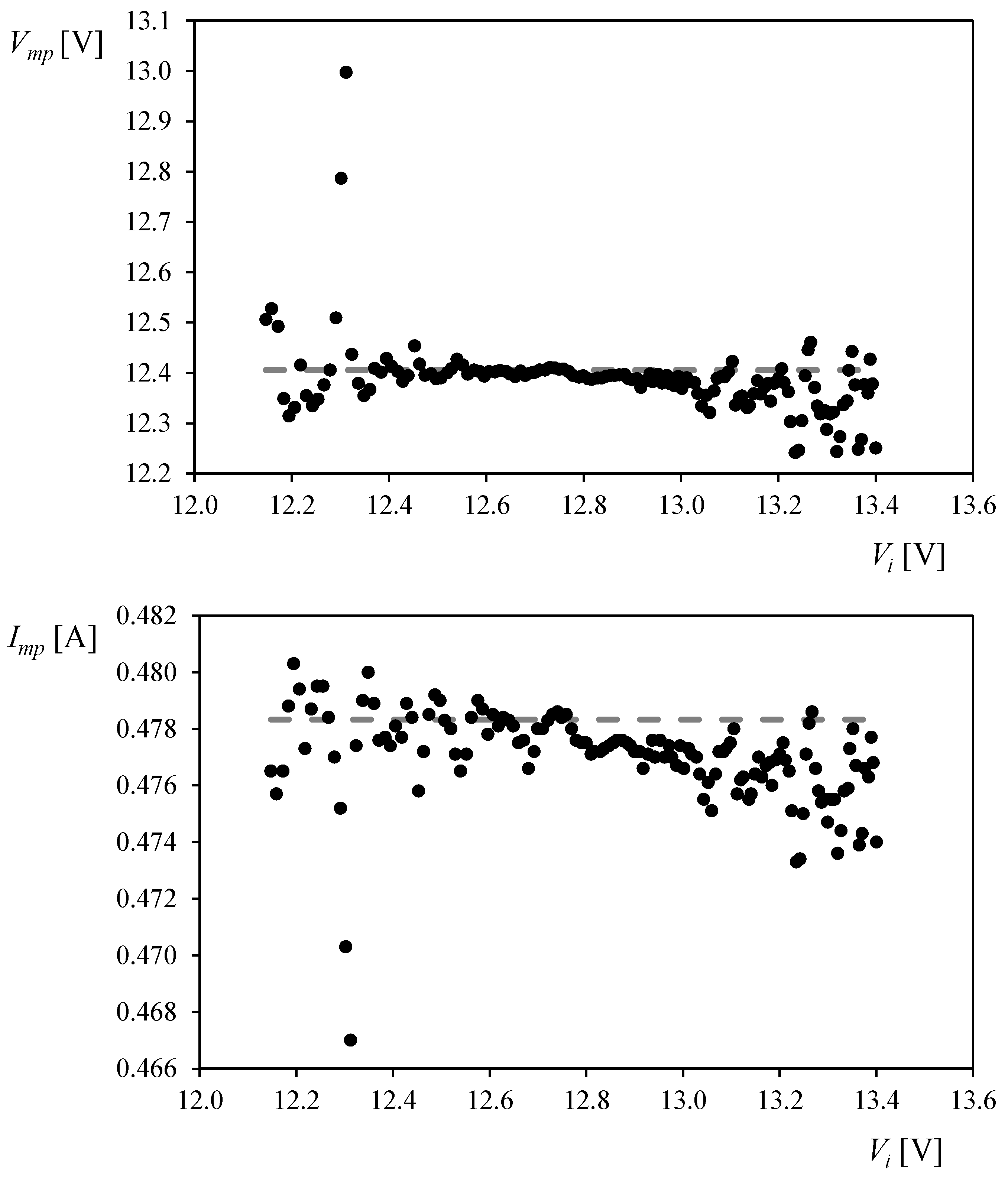
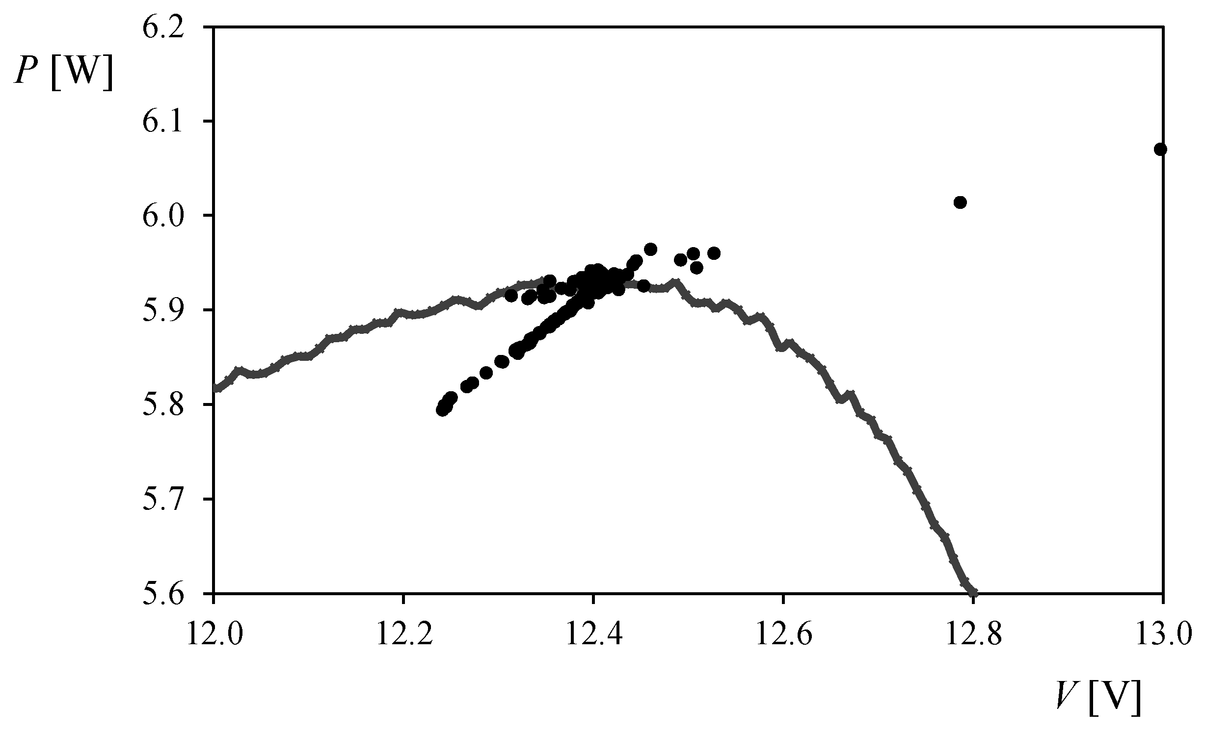
Once the equivalent circuit was calculated, it was used to predict the maximum power point. The calculated values of the maximum power voltage and current are included in Figure 6, and compared to the reference values extracted from experimental measurements. Results point out that the maximum power voltage is predicted quite accurately. Obviously, the best results are obtained with an operating point (Vi, Ii) closer to the reference MPP, particularly when this operating point is located to the right of this maximum. Furthermore, the local dispersion showed in the graphs from Figure 6 might be caused by the noise introduced in the calculation of the slope in each operation point (this slope is calculated with four points, the two closest at each side of the operation point). Finally, predictions of maximum power point (Vmp, Imp) compared to the P-V experimental curve are included in Figure 7.
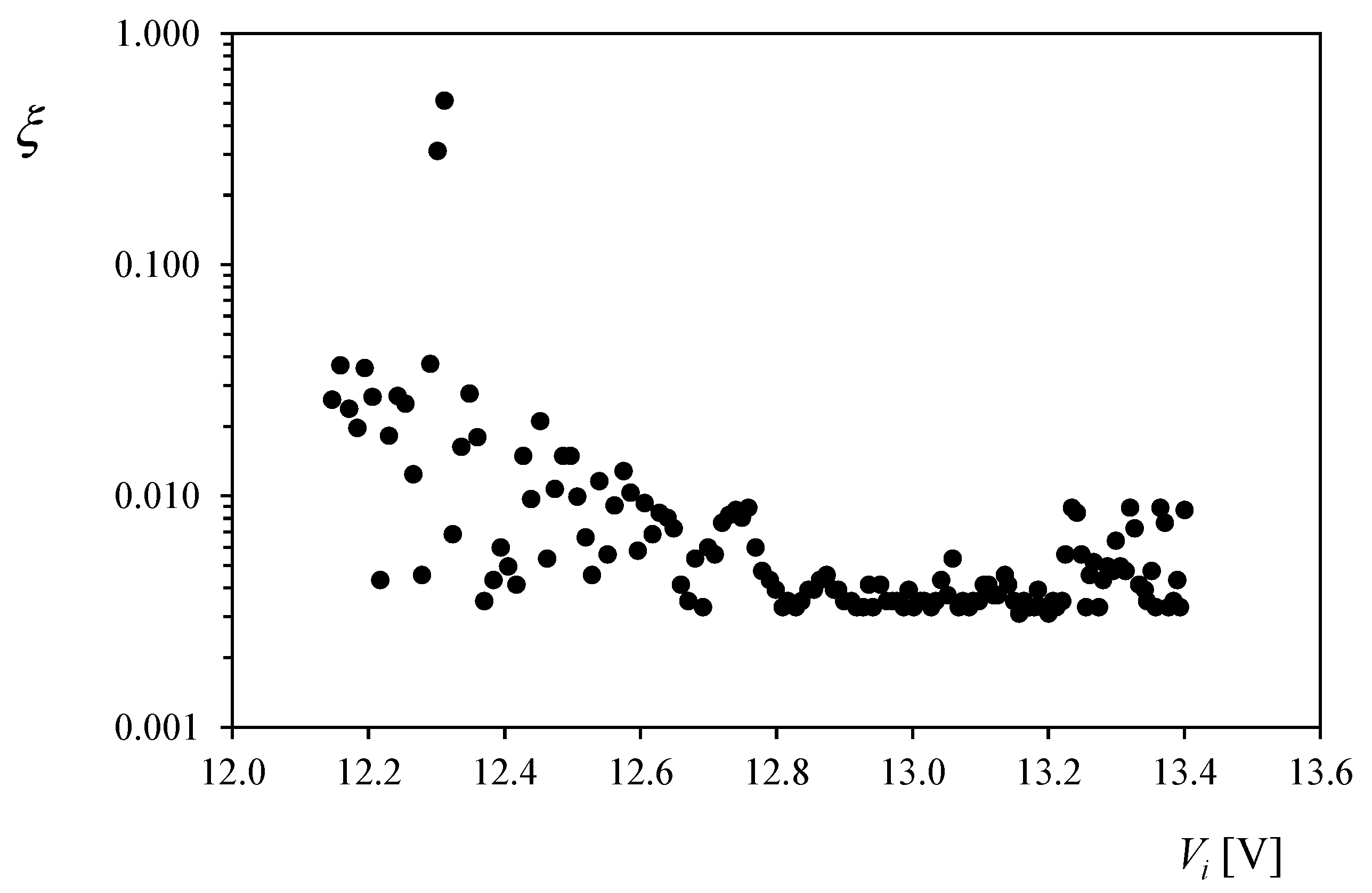
Additionally, in order to check the accuracy of the proposed methodology the normalized root mean square error, ξ (Equation (5)), has been used to evaluate the error between the I-V curve of the calculated equivalent circuits and the experimental data. Results (Figure 8) indicate a quite high accuracy levels, with ξ < 10−2 in almost all points, i, of the selected range (Vi ∈ [0.893·Voc, 0.985·Voc]). These figures agree with those normalized root mean squared error values calculated between the R.T.C. France solar cell and the Photowatt PWP201 solar panel experimental results, and the equivalent circuit models described in Section 1 (Table 2 and Table 3) and Section 3.1 (Table 4 and Table 5). It should also be pointed out that these results are also similar (better in some cases) than the ones obtained by other authors whose methods implied the use of the MPP to calculate the equivalent circuit parameters.
4. Conclusions
A new explicit analytical method for equivalent circuit parameter calculation is presented. This method allows calculating the equivalent circuit by knowing the short-circuit point and slope, the open-circuit point, and any other experimental point with its slope of the I-V curve.
Apart from its simplicity, the principal advantage of the method is that, contrary to other analytical methods, it is not necessary to know the maximum power point. Since this point is not easily obtainable experimentally, the proposed method can be very useful in reducing the data necessary for parameter determination. Furthermore, the accuracy of the results seems to be high, with a difference between experimental results of less than 1% in terms of current. The accuracy increases when the third point used for the calculation is nearby the maximum power point.
From the authors’ point of view, the simplicity and accuracy of these methods would make it interesting for end users with little calculation and testing resources. Also, the procedure described in the present work seems to be very appropriate for analyses that imply profuse calculations of equivalent circuits or determine initial values for numerical methods.
Finally, a MPPT method based in the analytical models has been proposed. Using the experimental data set of a solar panel, each measurement has been considered as an instantaneous operation point to be optimized. The value of this point, together with the value of the slope of the I-V curve at each point, has been used to predict the position of the maximum power point with quite high accuracy. The implementation of this methodology on the space power systems design works at IDR/UPM Institute is preliminary at present. Nevertheless, it represents a solid line of work as the accurate prediction of the maximum power point, with a small amount of information regarding the solar panel performance (short-circuit current and slope, open-circuit voltage, and operating point and slope), has been proven. Finally, it should be emphasized that an advantage of this method is the combination of the precision and feedback of online MPPT with the instantaneous reaction of offline methods.
Acknowledgments
The authors are indebted to Lorenzo Balenzategui, from CIEMAT, for his kind help and support regarding the UPMSat-2 solar panels’ testing activities. The authors are grateful to the Reviewers for their wise comments, which helped us to improve this work.
Author Contributions
Javier Cubas and Santiago Pindado developed the idea behind the present research, carrying also out the literature review and manuscript preparation at early stages. The methodology and analytic procedures were carried out by Javier Cubas. Final review, including final manuscript corrections, was done by Santiago Pindado and Felix Sorribes-Palmer. All authors were in charge of data generation/analysis and post-processing of the results.
Conflicts of Interest
The authors declare no conflict of interest.
References
- Jena, D.; Ramana, V.V. Modeling of photovoltaic system for uniform and non-uniform irradiance: A critical review. Renew. Sustain. Energy Rev. 2015, 52, 400–417. [Google Scholar] [CrossRef]
- Humada, A.M.; Hojabri, M.; Mekhilef, S.; Hamada, H.M. Solar cell parameters extraction based on single and double-diode models: A review. Renew. Sustain. Energy Rev. 2016, 56, 494–509. [Google Scholar] [CrossRef]
- Cubas, J.; Pindado, S.; Victoria, M. On the analytical approach for modeling photovoltaic systems behavior. J. Power Sources 2014, 247, 467–474. [Google Scholar] [CrossRef]
- Easwarakhanthan, T.; Bottin, J.; Bouhouch, I.; Boutrit, C. Nonlinear minimization algorithm for determining the solar cell parameters with microcomputers. Int. J. Sol. Energy 1986, 4, 1–12. [Google Scholar] [CrossRef]
- Cubas, J.; Pindado, S.; de Manuel, C. New method for analytical photovoltaic parameters identification: Meeting manufacturer’s datasheet for different ambient conditions. In International Congress on Energy Efficiency and Energy Related Materials (ENEFM2013); Oral, A.Y., Bahsi, Z.B., Ozer, M., Eds.; Springer International Publishing: Antalya, Turkey; Cham, Germany, 2014; pp. 161–169. [Google Scholar]
- Cubas, J.; Pindado, S.; Farrahi, A. New method for analytical photovoltaic parameter extraction. In Proceedings of the 2nd International Conference Renewable Energy Research Application (ICRERA 2013), Madrid, Spain, 20–23 October 2013; pp. 873–877. [Google Scholar]
- Pindado, S.; Cubas, J.; Sorribes-Palmer, F. On the harmonic analysis of cup anemometer rotation speed: A principle to monitor performance and maintenance status of rotating meteorological sensors. Measurement 2015, 73, 401–418. [Google Scholar] [CrossRef]
- Villalva, M.G.; Gazoli, J.R.; Filho, E.R. Modeling and circuit-based simulation of photovoltaic arrays. In Proceedings of the 2009 Brazilian Power Electronics Conference, Bonito-Mato Grosso do Sul, Brazil, 27 September–1 October 2009; pp. 1244–1254. [Google Scholar]
- Askarzadeh, A.; Rezazadeh, A. Parameter identification for solar cell models using harmony search-based algorithms. Sol. Energy 2012, 86, 3241–3249. [Google Scholar] [CrossRef]
- Askarzadeh, A.; Rezazadeh, A. Artificial bee swarm optimization algorithm for parameters identification of solar cell models. Appl. Energy 2013, 102, 943–949. [Google Scholar] [CrossRef]
- Lyden, S.; Haque, M.E. Maximum Power Point Tracking techniques for photovoltaic systems: A comprehensive review and comparative analysis. Renew. Sustain. Energy Rev. 2015, 52, 1504–1518. [Google Scholar] [CrossRef]
- Koutroulis, E.; Blaabjerg, F. Overview of maximum power point tracking techniques for photovoltaic energy production systems. Electr. Power Compon. Syst. 2015, 43, 1329–1351. [Google Scholar] [CrossRef]
- Verma, D.; Nema, S.; Shandilya, A.M.; Dash, S.K. Maximum power point tracking (MPPT) techniques: Recapitulation in solar photovoltaic systems. Renew. Sustain. Energy Rev. 2016, 54, 1018–1034. [Google Scholar] [CrossRef]
- Liu, L.; Meng, X.; Liu, C. A review of maximum power point tracking methods of PV power system at uniform and partial shading. Renew. Sustain. Energy Rev. 2016, 53, 1500–1507. [Google Scholar] [CrossRef]
- Cubas, J.; Pindado, S.; Sanz-Andrés, Á. Accurate simulation of MPPT methods performance when applied to commercial photovoltaic panels. Sci. World J. 2015, 2015, 1–16. [Google Scholar] [CrossRef] [PubMed]
- Laudani, A.; Riganti Fulginei, F.; Salvini, A. High performing extraction procedure for the one-diode model of a photovoltaic panel from experimental I–V curves by using reduced forms. Sol. Energy 2014, 103, 316–326. [Google Scholar] [CrossRef]
- Garrigós, A.; Blanes, J.M.; Carrasco, J.A.; Ejea, J.B. Real time estimation of photovoltaic modules characteristics and its application to maximum power point operation. Renew. Energy 2007, 32, 1059–1076. [Google Scholar] [CrossRef]
- Toledo, F.J.; Blanes, J.M.; Garrigós, A.; Martínez, J.A. Analytical resolution of the electrical four-parameters model of a photovoltaic module using small perturbation around the operating point. Renew. Energy 2012, 43, 83–89. [Google Scholar] [CrossRef]
- Blanes, J.M.; Toledo, F.J.; Montero, S.; Garrigós, A. In-site real-time photovoltaic I–V curves and maximum power point estimator. IEEE Trans. Power Electron. 2013, 28, 1234–1240. [Google Scholar] [CrossRef]
- Pindado Carrion, S.; Andres, S.; Franchini, S.; Pérez Grande, M.I.; Alonso, G.; Pérez, J.; Sorribes Palmer, F.; Cubas Cano, J.; García, A.; Roibás-Millán, E.; et al. Master in space systems, An advanced Master’ s Degree in space engineering. In Proceedings of the Athens ATINER’S Conference Paper Series No ENGEDU2016-1953, Athens, Greece, 9–12 May 2016; pp. 1–16. [Google Scholar]
- Pindado Carrion, S.; Roibás-Millán, E.; Cubas Cano, J.; García, A.; Sanz Andres, A.P.; Franchini, S.; Pérez Grande, M.I.; Alonso, G.; Pérez-Álvarez, J.; Sorribes Palmer, F.; et al. The UPMSat-2 Satellite: An academic project within aerospace engineering education. In Proceedings of the 2nd Annual International Conference on Engineering Education & Teaching, Atenas, Greece, 5–8 June 2017. [Google Scholar]
- Pindado, S.; Roibas, E.; Cubas, J.; Sorribes-Palmer, F.; Sanz-Andrés, A.; Franchini, S.; Grande, I.P.; Zamorano, J.; de la Puente, J.A.; Pérez-Álvarez, J.; et al. MUSE. Master in Space Systems at Universidad Politécnica de Madrid (UPM). 2017. Available online: https://www.researchgate.net/project/MUSE-Master-in-Space-Systems-at-Universidad-Politecnica-de-Madrid-UPM (accessed on 24 July 2017).
- Pindado, S.; Cubas, J. Simple mathematical approach to solar cell/panel behavior based on datasheet information. Renew. Energy 2017, 103, 729–738. [Google Scholar] [CrossRef]
- Roibás-Millán, E.; Alonso-Moragón, A.; Jiménez-Mateos, A.; Pindado, S. On solar panels testing for small-size satellites. The UPMSAT-2 mission. Meas. Sci. Technol. 2017. [Google Scholar]
- Barbini, N.; Lughi, V.; Mellit, A.; Pavan, A.M.; Tessarolo, A. On the impact of photovoltaic module characterization on the prediction of PV plant productivity. In Proceedings of the 9th International Conference Ecological Vehicles and Renewable Energies( EVER 2014), Montecarlo, Monaco, 25–27 March 2014. [Google Scholar]
- AlRashidi, M.R.; AlHajri, M.F.; El-Naggar, K.M.; Al-Othman, A.K. A new estimation approach for determining the I–V characteristics of solar cells. Sol. Energy 2011, 85, 1543–1550. [Google Scholar] [CrossRef]
- El-Naggar, K.M.; AlRashidi, M.R.; AlHajri, M.F.; Al-Othman, A.K. Simulated Annealing algorithm for photovoltaic parameters identification. Sol. Energy 2012, 86, 266–274. [Google Scholar] [CrossRef]
- Gong, W.; Cai, Z. Parameter extraction of solar cell models using repaired adaptive differential evolution. Sol. Energy 2013, 94, 209–220. [Google Scholar] [CrossRef]
- Peng, L.; Sun, Y.; Meng, Z.; Wang, Y.; Xu, Y. A new method for determining the characteristics of solar cells. J. Power Sources 2013, 227, 131–136. [Google Scholar] [CrossRef]
- Phang, J.C.H.; Chan, D.S.H.; Phillips, J.R. Accurate analytical method for the extraction of solar cell model parameters. Electron. Lett. 1984, 20, 406–408. [Google Scholar] [CrossRef]
- Bouzidi, K.; Chegaar, M.; Bouhemadou, A. Solar cells parameters evaluation considering the series and shunt resistance. Sol. Energy Mater. Sol. Cells 2007, 91, 1647–1651. [Google Scholar] [CrossRef]
- Wei, H.; Cong, J.; Lingyun, X.; Deyun, S. Extracting solar cell model parameters based on chaos particle swarm algorithm. In Proceedings of the 2011 International Conference on Electric Information and Control Engineering, Wuhan, China, 15–17 April 2011; pp. 398–402. [Google Scholar]
- Silva, J.P.; Balenzategui, J.L.; Nieto, M.B. On the relationship between spectral reflectance and working temperature of PV modules. In Proceedings of the 23rd European Photovoltaic Solar Energy Conference, Valencia, Spain, 1–5 September 2008; pp. 2861–2864. [Google Scholar]
- Silva, J.P.; Nofuentes, G.; Munoz, J.V. Spectral reflectance patterns of photovoltaic modules and their thermal effects. J. Sol. Energy Eng. ASME 2010, 132, 13. [Google Scholar] [CrossRef]
- Balenzategui, J.L.; Rodríguez-Outón, I.; Chenlo, F. Calibration of crystalline silicon solar cells as reference devices for cell testers and sorters. In Proceedings of the 25th European Photovoltaic Solar Energy Conference and Exhibition/5th World Conference Photovoltaic Energy Conversion, Valencia, Spain, 6–10 September 2010; pp. 2642–2648. [Google Scholar]
- Balenzategui, J.L.; Cuenca, J.; Rodríguez-Outón, I.; Chenlo, F. Intercomparison and validation of solar cell I-V characteristic measurement procedures. In Proceedings of the 27th European Photovoltaic Solar Energy Conference and Exhibition, Frankfurt, Gerermany, 25–27 September 2012; pp. 1471–1476. [Google Scholar]
Figure 1.
Four different equivalent circuit models: (a) 1-diode; (b) 1-diode/1-resistor; (c) 1-diode/2-resistor; (d) 2-diode/2-resistor [3].
Figure 1.
Four different equivalent circuit models: (a) 1-diode; (b) 1-diode/1-resistor; (c) 1-diode/2-resistor; (d) 2-diode/2-resistor [3].

Figure 2.
R.T.C. France silicon cell. (top): I-V curves (testing data and equivalent circuit models). (bottom): Accuracy of the equivalent circuit models.
Figure 2.
R.T.C. France silicon cell. (top): I-V curves (testing data and equivalent circuit models). (bottom): Accuracy of the equivalent circuit models.

Figure 3.
Photowatt PWP201 solar panel. (top): I-V curves (testing data and equivalent circuit models). (bottom): Accuracy of the equivalent circuit models.
Figure 3.
Photowatt PWP201 solar panel. (top): I-V curves (testing data and equivalent circuit models). (bottom): Accuracy of the equivalent circuit models.
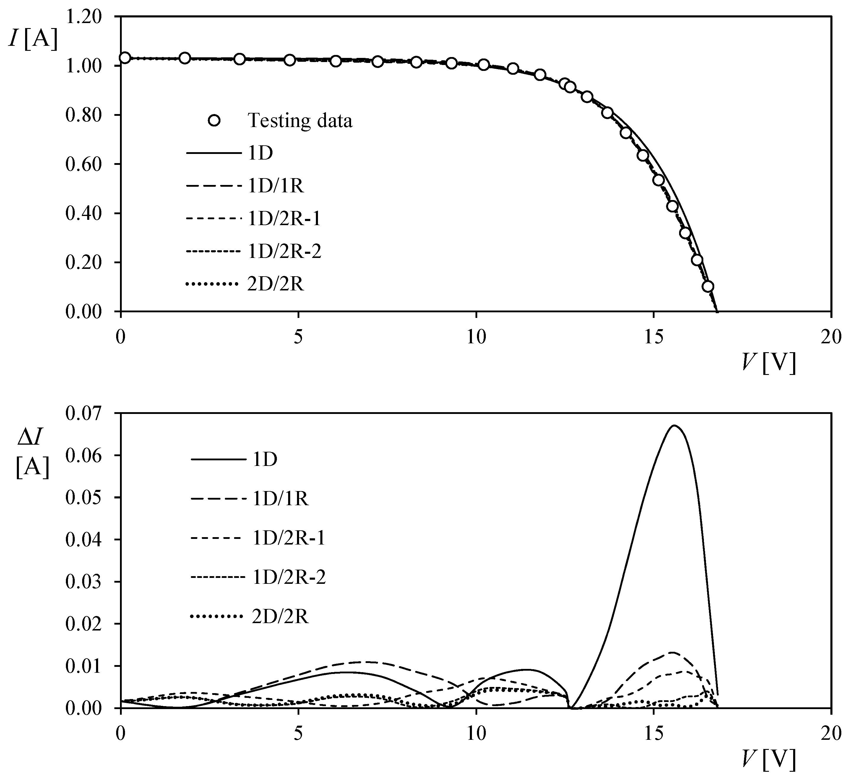
Figure 4.
SELEX Galileo 5-cell Photovoltaic Assembly.
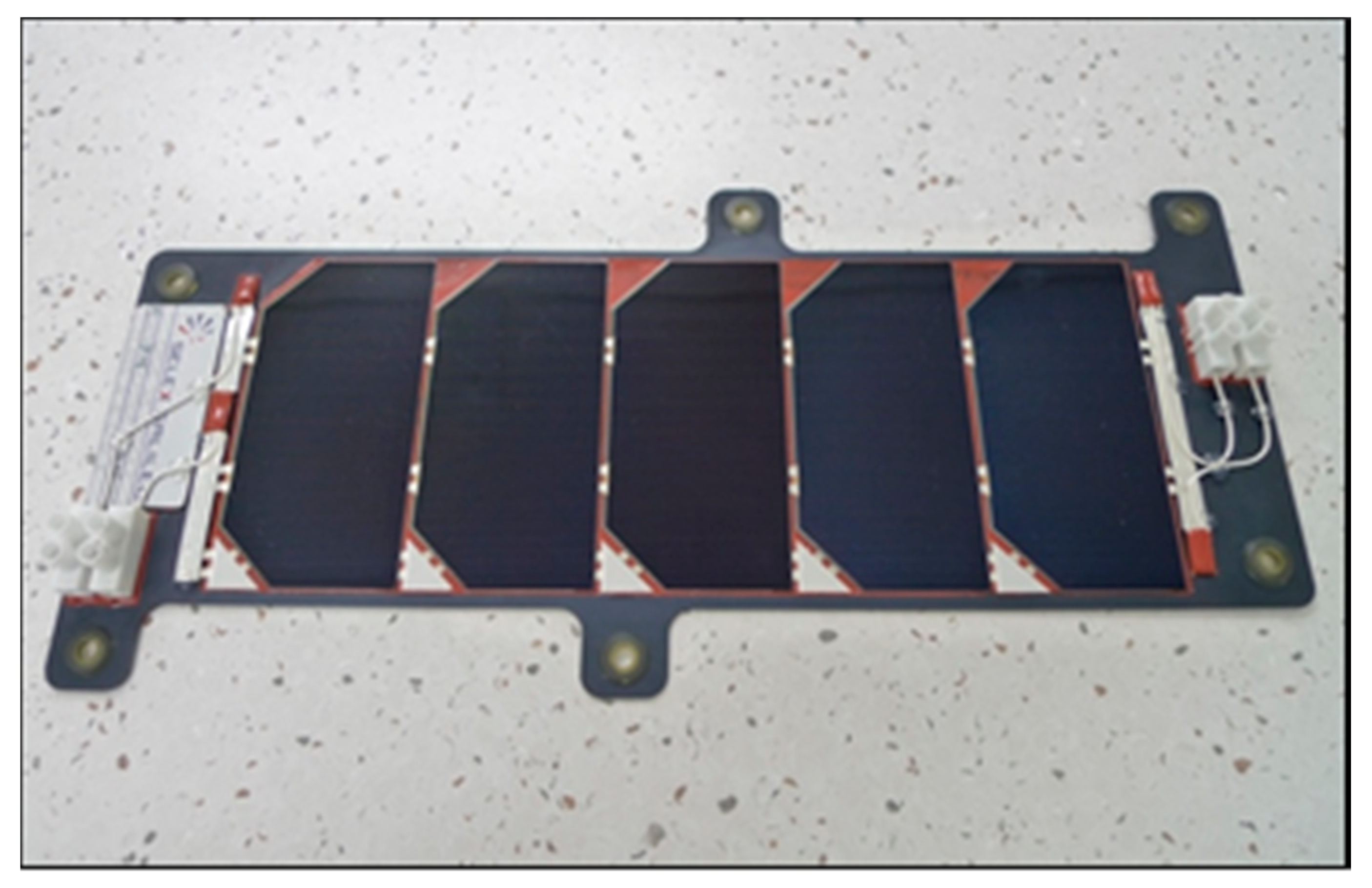
Figure 5.
I-V curve of a SELEX Galileo 5-cell Photovoltaic Assembly (see Figure 4). Starting from the measured values of Rsh0, Isc and Voc, each experimental point i: (Vi, Ii) measured between 0.893·Voc and 0.985·Voc was used as fictional operational point (this bracket was selected as it contains the maximum power point, Vmp = 0.927·Voc). Therefore, the equivalent circuit was calculated for each operational point following the procedure described in Section 2.
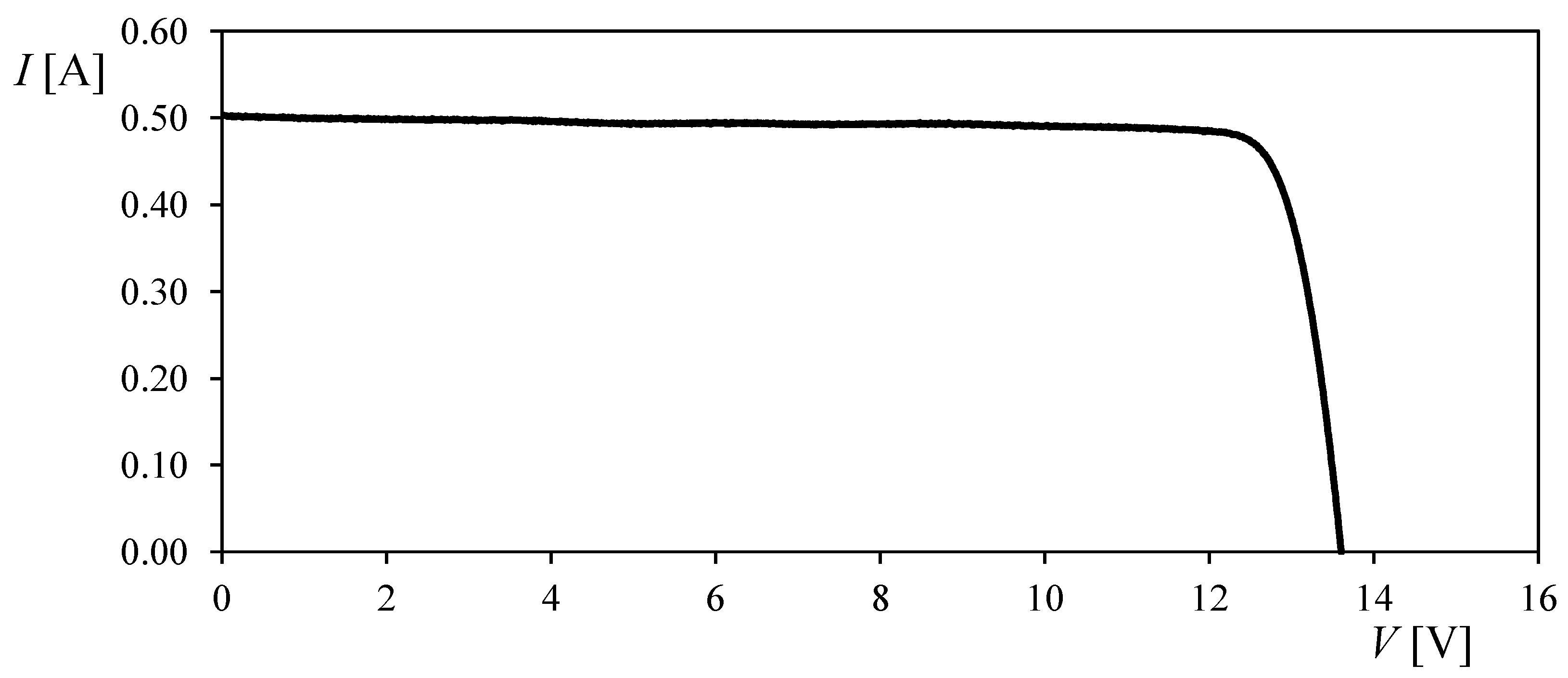
Figure 6.
Values of the maximum power voltage, Vmp, (top) and the maximum power current, Imp, (bottom), related to the equivalent circuit calculated with the proposed methodology. These variables are plotted (dots) as a function of the voltage level, Vi, at the operating point (Vi, Ii) selected for each circuit calculation. The experimental reference values of Vmp and Imp have been included in both graphs (dashed lines).

Figure 7.
Experimental P-V curve of the SELEX Galileo Photovoltaic Assembly (PVA) and location of the estimated maximum power points (Vmp, Imp) calculated with different operating points (Vi, Ii), using the proposed methodology.
Figure 7.
Experimental P-V curve of the SELEX Galileo Photovoltaic Assembly (PVA) and location of the estimated maximum power points (Vmp, Imp) calculated with different operating points (Vi, Ii), using the proposed methodology.

Figure 8.
Normalized RMSE, ξ, between the calculated and experimental I-V curves as a function of the voltage level, Vi, at the operating point (Vi, Ii) used in the estimation.
Figure 8.
Normalized RMSE, ξ, between the calculated and experimental I-V curves as a function of the voltage level, Vi, at the operating point (Vi, Ii) used in the estimation.

Table 1.
Characteristic data from R.T.C. France solar cell and Photowatt PWP201 solar panel.
| Characteristic Data | R.T.C. France | Photowatt PWP201 |
|---|---|---|
| Isc (A) | 0.7603 | 1.0300 |
| Voc (V) | 0.5728 | 16.778 |
| Vmp (V) | 0.4507 | 12.649 |
| Imp (A) | 0.6894 | 0.9120 |
| Rsh0 (Ω) | 246.80 * | 689.13 * |
| Rs0 (Ω) | 0.0907 * | 2.5193 * |
| T (K) | 306.15 | 318.15 |
| N | 1 | 36 |
* Estimated from data in [4].
Table 2.
Equivalent circuit parameters (see Figure 1, and Equations (1)–(4)) and normalized root mean square error (RMSE), ξ, in relation to the R.T.C. France solar cell.
Table 2.
Equivalent circuit parameters (see Figure 1, and Equations (1)–(4)) and normalized root mean square error (RMSE), ξ, in relation to the R.T.C. France solar cell.
| Model | Rs (Ω) | Rsh (Ω) | Ipv (A) | I01 (A) | a1 | I02 (A) | a2 | ξ |
|---|---|---|---|---|---|---|---|---|
| 1D | - | - | 0.7603 | 1.12 × 10⁻⁵ | 1.9509 | - | - | 2.25 × 10⁻² |
| 1D/1R | 0.0233 | - | 0.7603 | 2.07 × 10⁻⁶ | 1.6944 | - | - | 6.84 × 10⁻³ |
| 1D/2R-1 | 0.0481 | 28.931 | 0.7616 | 4.14 × 10⁻⁸ | 1.3 * | - | - | 5.95 × 10⁻³ |
| 1D/2R-2 | 0.0261 | 246.77 | 0.7604 | 1.44 × 10⁻⁶ | 1.6478 | - | - | 5.48 × 10⁻³ |
| 2D/2R | 0.0450 | 246.76 | 0.7604 | 1.54 × 10⁻⁹ | 1.1087 | 5.15 × 10⁻⁶ | 2.0 * | 2.50 × 10⁻³ |
* Selected as reasonable values for calculations.
Table 3.
Equivalent circuit parameters (see Figure 1, and Equations (1)–(4)) and normalized RMSE, ξ, in relation to the Photowatt PWP201 solar panel.
Table 3.
Equivalent circuit parameters (see Figure 1, and Equations (1)–(4)) and normalized RMSE, ξ, in relation to the Photowatt PWP201 solar panel.
| Model | Rs (Ω) | Rsh (Ω) | Ipv (A) | I01 (A) | a1 | I02 (A) | a2 | ξ |
|---|---|---|---|---|---|---|---|---|
| 1D | - | - | 1.0300 | 1.55 × 10⁻⁴ | 1.9319 | - | - | 2.87 × 10⁻² |
| 1D/1R | 0.8884 | - | 1.0300 | 1.80 × 10⁻⁵ | 1.5520 | - | - | 6.70 × 10⁻³ |
| 1D/2R-1 | 1.4429 | 497.75 | 1.0330 | 7.04 × 10⁻⁷ | 1.2 * | - | - | 4.59 × 10⁻³ |
| 1D/2R-2 | 1.2829 | 687.85 | 1.0319 | 2.04 × 10⁻⁶ | 1.2968 | - | - | 2.31 × 10⁻³ |
| 2D/2R | 1.2004 | 687.93 | 1.0318 | 5.31 × 10⁻⁶ | 1.3882 | −1.96 × 10⁻⁵ | 2.0 * | 2.04 × 10⁻³ |
* Selected as reasonable values for calculations.
Table 4.
Equivalent circuit parameters and normalized RMSE, ξ, extracted with the present method (P.M.) in relation to the R.T.C. France solar cell.
Table 4.
Equivalent circuit parameters and normalized RMSE, ξ, extracted with the present method (P.M.) in relation to the R.T.C. France solar cell.
| Model | Rs (Ω) | Rsh (Ω) | Ipv (A) | I0 (A) | a | ξ |
|---|---|---|---|---|---|---|
| P.M. 1 * | 0.0459 | 246.78 | 0.7606 | 2.92 × 10⁻⁶ | 1.7407 | 1.24 × 10⁻² |
| P.M. 2 ** | 0.0403 | 246.76 | 0.7606 | 5.02 × 10⁻⁷ | 1.5283 | 3.60 × 10⁻³ |
| Al-Rashidi et al. [26] | 0.0313 | 64.103 | 0.7617 | 9.98 × 10⁻⁷ | 1.6 | 2.509 × 10⁻² |
| El-Naggar et al. [27] | 0.0345 | 43.103 | 0.762 | 4.767 × 10⁻⁷ | 1.5172 | 2.235 × 10⁻³ |
| Gong and Cai [28] | 0.0364 | 53.719 | 0.7608 | 3.23 × 10⁻⁷ | 1.4812 | 1.297 × 10⁻³ |
| Askarzadeh and Rezazadeh [9] | 0.0366 | 53.595 | 0.7607 | 3.05 × 10⁻⁷ | 1.4754 | 1.308 × 10⁻³ |
| Peng et al. [29] | 0.0364 | 54.054 | 0.7609 | 3.22 × 10⁻⁷ | 1.4837 | 4.659 × 10⁻³ |
| Askarzadeh and Rezazadeh [10] | 0.0366 | 52.290 | 0.7608 | 3.06 × 10⁻⁷ | 1.4758 | 1.303 × 10⁻³ |
| Laudani et al. [16] | 0.0368 | 49.9736 | 0.7611 | 2.0901 × 10⁻⁷ | 1.4701 | 1.163 × 10⁻³ |
* Point 1; ** Point 2.
Table 5.
Equivalent circuit parameters and normalized RMSE, ξ, extracted with the present method (P.M.) in relation to the Photowatt PWP201 solar panel.
Table 5.
Equivalent circuit parameters and normalized RMSE, ξ, extracted with the present method (P.M.) in relation to the Photowatt PWP201 solar panel.
| Model | Rs (Ω) | Rsh (Ω) | Ipv (A) | I0 (A) | a | ξ |
|---|---|---|---|---|---|---|
| P.M. 1 * | 1.7146 | 687.42 | 1.0343 | 3.105 × 10⁻⁷ | 1.1342 | 1.24 × 10⁻² |
| P.M. 2 ** | 1.3995 | 687.73 | 1.0338 | 1.260 × 10⁻⁶ | 1.2512 | 4.00 × 10⁻³ |
| Phang et al. [30] | 0.0832 | 561.03 | 1.0319 | 6.405 × 10⁻⁵ | 1.7602 | 2.05 × 10⁻² |
| Bouzidi et al. [31] | 1.2030 | 555.55 | 1.0339 | 3.076 × 10⁻⁶ | 13385 | 5.53 × 10⁻³ |
| Wei et al. [32] | 1.0755 | 1850.1 | 1.0286 | 8.301 × 10⁻⁶ | 1.4512 | 4.04 × 10⁻³ |
| Al-Rashidi et al. [26] | 1.1968 | 555.55 | 1.0441 | 3.436 × 10⁻⁶ | 1.3496 | 2.22 × 10⁻³ |
| El-Naggar et al. [27] | 1.1989 | 833.33 | 1.0331 | 3.664 × 10⁻⁶ | 1.3561 | 2.44 × 10⁻³ |
| Gong and Cai [28] | 1.2013 | 981.98 | 1.0305 | 3.482 × 10⁻⁶ | 1.3512 | 2.02 × 10⁻³ |
| Peng et al.[29] | 1.2132 | 625.00 | 1.0313 | 3.221 × 10⁻⁶ | 1.3423 | 7.49 × 10⁻³ |
| Cubas et al. [3] | 1.3535 | 559.68 | 1.0342 | 1.321 × 10⁻⁶ | 1.2554 | 2.86 × 10⁻³ |
| Laudani et al. [16] | 1.2241 | 689.32 | 1.3354 | 2.826 × 10⁻⁶ | 1.3294 | 2.09 × 10⁻³ |
* Point 1; ** Point 2.
© 2017 by the authors. Licensee MDPI, Basel, Switzerland. This article is an open access article distributed under the terms and conditions of the Creative Commons Attribution (CC BY) license (http://creativecommons.org/licenses/by/4.0/).
Share and Cite
MDPI and ACS Style
Cubas, J.; Pindado, S.; Sorribes-Palmer, F. Analytical Calculation of Photovoltaic Systems Maximum Power Point (MPP) Based on the Operation Point. Appl. Sci. 2017, 7, 870. https://doi.org/10.3390/app7090870
AMA Style
Cubas J, Pindado S, Sorribes-Palmer F. Analytical Calculation of Photovoltaic Systems Maximum Power Point (MPP) Based on the Operation Point. Applied Sciences. 2017; 7(9):870. https://doi.org/10.3390/app7090870
Chicago/Turabian StyleCubas, Javier, Santiago Pindado, and Felix Sorribes-Palmer. 2017. "Analytical Calculation of Photovoltaic Systems Maximum Power Point (MPP) Based on the Operation Point" Applied Sciences 7, no. 9: 870. https://doi.org/10.3390/app7090870
Note that from the first issue of 2016, this journal uses article numbers instead of page numbers. See further details here.