Article

Analysis Method of Articulated Torque of Heavy-Duty Six-Legged Robot under Its Quadrangular Gait

1
College of Mechanical Engineering, Tianjin University of Technology and Education, Tianjin 300222, China
2
State Key Laboratory of Robotics and System, Harbin Institute of Technology, Harbin 150001, China
*
Authors to whom correspondence should be addressed.
Appl. Sci. 2016, 6(11), 323; https://doi.org/10.3390/app6110323
Submission received: 19 September 2016 / Revised: 20 October 2016 / Accepted: 25 October 2016 / Published: 28 October 2016

Abstract

:
The articulated torque is an important base for developing heavy-duty multi-legged robots. To quickly obtain accurate articulated torques, a method is presented for an electrically driven heavy-duty six-legged robot under its quadrangular gait. First, the typical walking ways and the working conditions of support phase are analyzed. The static articulated torques are solved though Matrix Laboratory (MATLAB) software. The variable tendency charts of torques are acquired with the changes in the joint angles. The static simulation of robot is carried out by Automatic Dynamic Analysis of Mechanical Systems (ADAMS) software. A comparative analysis of the maximum static articulated torques shows that the theoretical calculation values are smaller than the static simulation values. The maximum error value is about 5%. Finally, a prototype of the electrically driven heavy-duty six-legged robot is developed. Its climbing experiments prove that the proposed method can be applied to quickly determine accurate articulated torques.

1. Introduction

With the development of robotics, many intelligent walking robots are widely applied in the life of human [1], outdoor exploration [2,3], and so on. Intelligence [4], high trafficability [5], low energy dissipation [6,7], and high load rate [8] are generally viewed as parts of the important development directions for ground walking roots. The ground walking robots have many types, including wheeled type, tracked type, legged type, snake type, etc. The multi-legged robot has attracted the attention of researchers because of its excellent features in trafficability and flexibility. Based on the development history of multi-legged robots [9,10], we can find that the multi-legged robots, especially the heavy-duty multi-legged robots, not only the academic research and practical application have generally come later than for the wheeled robots, but also have much lower depth and breadth of research than the wheeled robots.
Many researchers mainly focus on the gait planning [11,12] and motion control [13,14,15,16] in the research on the multi-legged robots. They do not care about the torques of joints. Their prototypes generally have a small structure and light mass [11,17]. Based on non-actual limiting poses of robot, the extremal estimation method is employed to roughly estimate the articulated torques of the legged robot. Then, a very large safety margin is produced for the torques of joints. It is not conducive to reducing the mass and energy dissipation of robot. Therefore, it is necessary to select a reasonably calculation method of the articulated torques for the multi-legged robots, especially for the heavy-duty multi-legged robots.
Erden and Leblebicioğlu [18] carried out the research of the torque distribution for a six-legged robot. The articulated torques were regarded as the variables to constructed the dynamic formulation. The minimization of the articulated torque was implemented based on the quadratic objective function of the torque of joint. According to the Denavit–Hartenberg notations and the Lagrange–Euler formulation, Roy et al. [19] selected the least squared method to carry out the estimation of optimal feet force and articulated torques for a six-legged robot. Santos et al. [20] made a detailed study on the articulated torque, energy dissipation, and stability for a six-legged robot. Through the research by Santos’ team, we can obtain that the middle legs have the maximum torques of joints when the robot walks by the ant-type tripod gait. Silva and his team [21] gave the dynamic model of a hexapod robot, and that model referred to the torques of joints. The quadratic integral of articulated torque could be viewed as the index of energy dissipation. Although the methods mentioned above can effectively obtain the articulated torques of multi-legged robots, they either refer to a large number of calculations, or relate to multiple derivations, or involve complex mathematic expressions, which brings certain difficulties to some researchers. Hence, those methods are limited in the practical development of multi-legged robots.
Due to the complex of theoretical analysis on solving the articulated torques of the legged robots, ADAMS (Automatic Dynamic Analysis of Mechanical Systems) software [22] is widely selected to carry out the simulation analysis by many researchers. Based on the help files of ADAMS software, it can be obtained that the contact is set to the spring-damping model between one object and another. Then, it is very easy to bring the unsuitable contact parameters from operators to ADAMS software. The larger impact and slip phenomenon would occur between the feet and the ground, which results in reducing the reference of the simulation data of articulated torques. Therefore, Mahapatra [22], Wang [23], et al. only perform the simulation analysis of the multi-legged robots on the flat terrains.
Based on the above problems and the previous research [24,25,26,27], an analysis method of articulated torque is brought forward, when the equivalence is executed from the legs of the support phase to the middle line of symmetry. Then, an electrically driven heavy-duty six-legged robot under the quadrangular gait is introduced for presenting the above analysis method. To reduce the mass of robot and improve the load ratio, it needs to reasonably design the configuration and mobile way of robot. Meanwhile, it is necessary to avoid the same joint not only suffering a larger rotating speed but also undertaking a larger articulated torque. Thus, the tripod gait can be employed to carry out the maximum walking speed of robot on the flat terrain. The quadrangular gait can be used to climb the maximum slope for the electrically driven heavy-duty six-legged robot. According to the articulated torques under the quadrangular gait and articulated rotating speeds under the tripod gait, the drive devices and actuating devices of joints can be reasonably selected, respectively.
Based on the quadrangular gait, the analysis method of articulated torque is elaborated for the heavy-duty six-legged robot in this article. This article is divided into six sections. In Section 2, the walking ways of heavy-duty six-legged robot is analyzing under the quadrangular gait. The highly stable swing sequences of legs are obtained when the robot overpasses the slope. Based on the crab-type quadrangular gait, the typical working conditions of the support phase are gained. In Section 3, the normal contact forces and static articulated torques are, respectively, solved under the typical working conditions of the support phase. According to their variable tendency charts, the maximum values are obtained. In Section 4, the static simulation is executed based on the pose of the robot under the maximum articulated torques. The simulation curves are acquired about the normal contact forces and articulated torques. A comparison of the theoretical calculation values and the simulation values is performed. In Section 5, a prototype of the electrically driven heavy-duty six-legged robot is developed. The climbing experiments of robot are carried out. In the final section, the conclusions are presented.

2. Walking Ways of Heavy-Duty Six-Legged Robot under Quadrangular Gait

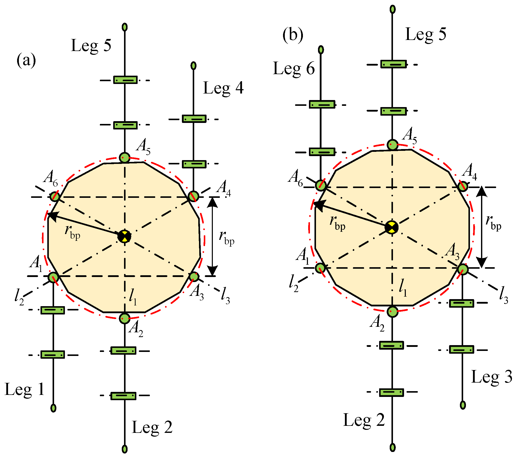
2.1. Typical Walking Ways of Robot under Quadrangular Gait

To conveniently execute the analysis of the articulated torques, the electrically driven heavy-duty six-legged robot is called the heavy-duty six-legged robot for short. The mechanism of robot and the structure of leg are shown in Figure 1. Every leg of the robot has three joints, including an abductor joint, hip joint, and knee joint. The axes of the abductor joints follow the direction of z-axis. The axes of the hip joints and knee joints run parallel to the y-axis. Based on Figure 1, it can be concluded that the mass of robot is mainly undertaken by the hip joints and knee joints. The maximum walking speed can be achieved by the abductor joint. Thus, the drive devices and actuating devices need to output large articulated toque for the hip joints and knee joints, and to output large rotating speed for the abductor joints.
In Figure 1, the abductor joint, hip joint, and knee joint are, respectively, defined as Ai, Hi, Ki (i = 1, …, 6). The lengths of the coxa, thigh, and shin, respectively, set as lc, lt and ls. The included angle between the coxa of leg i and the thigh of leg i is defined as βi′ (i = 1, …, 6). βi (i = 1, …, 6) is regarded as the included angle between the coxa of leg i and the shin of leg i. The relations between βi′ and βi are 0° ≤ βi′ ≤ βi ≤ 90°. The body coordinate system of robot is set as B ; it locates at the center of body. The gravity vector and the principal moment of the robot are, respectively, defined as FB and MB. The abductor joint coordinate system of leg i contains z 1 ( i ) axis, x 1 ( i ) axis, and y 1 ( i ) axis. The z 1 ( i ) axis is parallel to the ZB axis. The x 1 ( i ) axis keeps parallel with the coxa of leg i. The leg i lies in the plan z 1 ( i ) x 1 ( i ) . The foot coordinate systems o i and f i of leg i are, respectively, parallel to the body coordinate system B and the abductor joint coordinate system of leg i. G expresses the coordinate system of ground.
Four kinds of typical waking ways under the quadrangular gait can be obtained for the heavy-duty six-legged robot (Figure 2). In Figure 2, the straight lines l1, l2 and l3 are orthogonal to the relevant axes of abductor joints. θi′ and θi (i = 1, …, 6) are defined as the rotation angles of the abductor joint under the crab type and ant type walking ways, respectively.
One period of the quadrangular gait contains three steps: 1/3 gait, 2/3 gait and 3/3 gait (it represents the last 1/3 gait). When the stability and articulated torques are not considered for the heavy-duty six-legged robot, the sum of swing sequences of the legs is 720 kinds under the quadrangular gait. Whereas, when the robot traverses a slope, it is necessary to consider the stability and articulated torques. The number of the support phase legs should be two for the rear and front legs, respectively. Then, the total swing sequences of the legs are 36 kinds. Based on the configuration of robot, 18 kinds of the higher-stable swing sequences of the legs can be obtained under the quadrangular gait to pass a slope (Table 1).
Based on Figure 1 and Figure 2a, the expressions of the tangential forces of feet can be gained for legs 1, 2, 3, 4, 5 and 6 when the value of θi′ is zero. Thus,
( F x 1 F x 2 F x 3 F x 4 F x 5 F x 6 ) = ( F x ( f 1 ) F x ( f 2 ) F x ( f 3 ) F x ( f 4 ) F x ( f 5 ) F x ( f 6 ) )
Based on Figure 2, it can be concluded that the crab–ant mixed type I and crab–ant mixed type II can be transformed from the crab type or the ant type. Generally, we all know that the rearmost leg of robot experiences the maximum normal contact force when the robot passes along a slope. Then, the joints of the rearmost leg have the maximum values of torques in the homogeneous joints. According to the structure of leg and four kinds of typical walking ways, it can be concluded that the large static torques of the hip joint and knee joint can be obtained when the crab-type quadrangular gait is selected to overpass a slope. Thus, the support phase of the crab-type quadrangular gait can be only analyzed for gaining the torques of the hip joints and knee joints.

2.2. Support Phase Analysis of Crab-Type Quadrangular Gait

The crab-type quadrangular gait is employed to overpass a slope for the heavy-duty six-legged robot, as shown in Figure 3. The three kinds of typical working conditions of the support phase are gained based on the crab-type quadrangular gait, the rotation angle θi′ of 0°, and Table 1: working condition I, II and III. In working condition I, the support phase contains legs 1, 3, 4 and 6, as shown in Figure 4. In working condition II, the support phase includes legs 1, 2, 4 and 5, or legs 2, 3, 5 and 6, as shown in Figure 5. In working condition III, the support phase comprises legs 1, 2, 4 and 6, or legs 2, 3, 4 and 6, or legs 1, 3, 4 and 5, or legs 1, 3, 5 and 6, as shown in Figure 6.
Based on Figure 4, Figure 5 and Figure 6, the working condition III can be viewed as a combination by the working conditions I and II. The state effects of the support phases in Figure 6a,b are equal to each other; they are defined as working condition III-1. The state effect of the support phase in Figure 6c is same as that in Figure 6d; they are named working condition III-2.
A variable w, referring to the typical working conditions I, II, III-1 and III-2, is introduced for analyzing the articulated torques of robot. The active forces from the ground to the foothold of leg i are, respectively, defined as Fwxi, Fwyi and Fwzi in three directions. The static torques of the hip joint and knee joint of the leg i are, respectively, regarded as Mwhi and Mwki. Fewxj, Fewyj and Fewzj represent the active forces of equivalent leg j (j =1, …, 6) from the ground in three directions. Mewhj and Mewkj are the static articulated torques of equivalent leg j for the hip joint and knee joint.
Based on the above analysis, the rearmost leg in the support phase has the maximum torques of the hip joint and knee joint when the rotation angle θi′ is zero. The static torques of the hip joint and knee joint of leg i mainly depend on Fzi and Fxi. Fyi can be approximately ignored because of little influence on solving the torques of joints. To make it easier to explain the analysis of the static articulated torques, it is to assume that the homogeneous joints in the same phase have the equal rotation angles of the joints. The bottom surface of bearing platform keeps parallel with the slope.
To discuss the analysis method of the torque of joint in this paper, some parameters of robot are assumed. For example, the mass of the robot is supposed to be 250 kg. The mass of the rated load is presumed to be 50 kg. The total mass of one leg is assumed to be 25 kg, including the mass mc of one coxa, the mass mt of one thigh and the mass ms of one shin. Meanwhile, mc includes the mass of the driving device and actuating device for one abductor joint. mt contains the mass of the driving devices and actuating devices for one hip joint and one knee joint. According to Figure 2b and the maximum distance from the gravity center of bearing platform to the ground, the effective dimensions of robot are about 1.2 m × 1.2 m × 1.0 m. αi is the angle of the slope, whose value is assumed to range from 0° to 34.8° based on the requirements of working condition. The maximum walking speed of robot is about 0.1 m/s on the flat terrain. The robot is allowed to select a lower walking speed to overpass the slope.

3. Static Torque Analysis of Hip Joint and Knee Joint

When the homogenous joints have the equal rotation angles in the same phase, the hip joint and knee joint of the rearmost leg have the maximum static torques on a slope. Due to the low walking speed of robot, the moments of inertia are ignored in the torque analysis of the joint. Thus, the static torques of joints can be regarded as a basis to match their driving devices and actuating devices. The support phase is only considered in the analysis of the static articulated torque. The transfer phase is ignored, and its weight is viewed as a load to add to the gravity center of the bearing platform. To quickly acquire accurate torques of the hip joint and knee joint, the statics and equivalence means are employed. Based on the rotation angle θi′ of 0° and the crab-type quadrangle gait, the support phases are analyzed under the working conditions I, II, III-1 and III-2. The static torques of the hip joint and knee joint are solved when the heavy-duty six-legged robot traverses the maximum slope.

3.1. Analysis of Static Articulated Torques under Working Condition I

Based on Figure 4, legs 1, 3, 4 and 6 are parallel to the straight line l1. It is deduced that the poses of legs 1 and 3 are equal to each other. The pose of leg 4 is the same as the pose of leg 6. The equivalences are respectively carried out through legs 1, 3, 4 and 6 to the straight line l1. The equivalent legs are obtained and shown in Figure 7. Thus, the pose of the equivalent leg 1I is equal to the poses of legs 1 and 3. The pose of the equivalent leg 4I is equal to the poses of legs 4 and 6. According to the poses of legs in the support phase, it can be concluded that the moments of couples caused by the equivalence are mutually offset. The maximum static torques of the hip joint and knee joint can be obtained. Under a stable condition of the heavy-duty six-legged robot, the rotation angles of the homogeneous joints are equal. Then, the relations can be acquired: β′1,3 = β′4,6 = β1′ = β3′ = β4′ = β6′ and β1,3 = β4,6 = β1 = β3 = β4 = β6.
According to Figure 3, Figure 4 and Figure 7, the relations can be obtained: FIz1 = FIz3 = FeIz1/2, MIh1 = MIh3 and MIk1 = MIk3. The mathematical expression of torque is written for the foothold oeI4. The normal contact force FeIz1 can be solved. Then,
G sin α i × l IG x G cos α i × l IG z + F eI z 1 × l eI z 1 = 0
where
  • l IG x = l t sin β 1 , 3 + l s sin β 1 , 3
  • l IG z = r bp / 2 + l c + l t cos β 1 , 3 + l s cos β 1 , 3
  • l eI z 1 = 2 ( l c + l t cos β 1 , 3 + l s cos β 1 , 3 ) + r bp
G is the weight of the robot and rated load; rbp is the effective radius of the bearing platform; lIGx is the distance from the vector of the G component along the direction of XG to the foothold oeI4; lIGz is the distance from the vector of the G component along the direction of ZG to the foothold oeI4; and leIz1 is the distance from the vector of FeIz1 to the foothold oeI4.
Through FeIz1 and the right-handed rule for judging the sign of the articulated torque, the mathematical expression can be written for the static torque MIh1 of hip joint of leg 1 and the static torque MIk1 of knee joint of leg 1. Thus,
M = F I z 1 l I z 1 F I x 1 l I x 1 G t l IGt G s l IGs
where
  • M = ( M Ih 1 M Ik 1 )
  • l I z 1 = ( l t cos β 1 , 3 + l s cos β 1 , 3 l s cos β 1 , 3 )
  • l I x 1 = ( l t sin β 1 , 3 + l s sin β 1 , 3 l s sin β 1 , 3 )
  • l IGt = ( l t cos ( α i + β 1 , 3 ) / 2 0 )
  • l IGs = ( l t cos ( α i + β 1 , 3 ) + l s cos ( α i + β 1 , 3 ) / 2 l s cos ( α i + β 1 , 3 ) / 2 )
  • F I z 1 = F eI z 1 / 2
  • F I x 1 = F eI x 1 / 2 G sin α i / 4
where M is the matrix of the articulated torque, lIz1 is the matrix of the distance from the vector of FIz1 to the axes of the hip joint and knee joint of leg 1, lIx1 is the matrix of the distance from the vector of FIx1 to the axes of the hip joint and knee joint of leg 1, Gt is the weight of the thigh, lIGt is the matrix of the distance from the vector of Gt to the axes of the hip joint and knee joint of leg 1, Gs is the weight of the shin, lIGs is the matrix of the distance from the vector of Gs to the axes of the hip joint and knee joint of leg 1, FIz1 is the normal contact force of foothold of leg 1, and FIx1 is the force of foothold of leg 1 in the direction XG.
According to the practical working condition I, the constrained conditions of leg 1 are Gcos αi/4 ≤ FIz1Gcos αi/2 and 0° ≤ βi′ ≤ βi ≤ 90°. Based on Equations (2) and (3), and the above constrained conditions, MATLAB (Matrix Laboratory) software (MATLAB R2010b, MathWorks Inc., Natick, MA, USA) is employed to solve the normal contact force FIz1, static torque MIh1 of the hip joint, and static torque MIk1 of the knee joint of leg 1; their variable tendency charts with changes in β′i and βi are, respectively, shown in Figure 8, Figure 9 and Figure 10.
Figure 8 shows that the maximum value of FIz1 is 1204.00 N when the included angles βi′ and βi are 62° and 85°, respectively. The minimum value of FIz1 is 602.10 N when the values of included angles are zero for βi′ and βi. Figure 9 shows that the maximum value of positive static torque MIh1+ is 529.80 N·m when the values of included angles are zero for βi′ and βi. The maximum value of negative static torque MIh1− is 48.18 N·m when the values of included angles βi′ and βi are 57° and 90°, respectively. Figure 10 shows that the maximum value of positive static torque MIk1+ is 285.00 N·m when the values of included angles are zero for βi′ and βi. The maximum value of negative static torque MIk1− is 199.50 N·m when the value of included angle βi is 90° and the value of included angle βi′ can range from 0° to 57°. Based on Figure 8, Figure 9 and Figure 10, it is deduced that the effective poses of the heavy-duty six-legged robot are limited by the hip joints and knee joints. Under the wording condition I to pass the maximum slope, the included angle βi′ of the hip joint and the included angle βi of the knee joint should meet the conditions: 0° ≤ βi′ ≤ βi ≤ 90° and 0° ≤ βi′ + βi ≤ 147°.

3.2. Analysis of Static Articulated Torques under Working Condition II

Based on Figure 5a, the method of equivalence is employed to solve the static torques of the hip joint and knee joint. Then, the forces FIIz1 and FIIx1 of leg 1 are carried out the equivalence to leg 2. The forces FIIz4 and FIIx4 of leg 4 are implemented the equivalence to leg 5. The equivalent model is shown in Figure 11. When the equivalence of the force FIIx1 is executed to leg 2, the force FIIx2 becomes the force FeIIx2. The moment of couple MIIx1-2 is obtained. When the equivalence of the force FIIz1 is performed to leg 2, the force FIIz2 becomes the force FeIIz2. The moment of couple MIIz1-2 is acquired. When the equivalence of the force FIIx4 is actualized to leg 5, the force FIIx5 becomes the force FeIIx5. The moment of couple MIIx4-5 is gained. When the equivalence of the force FIIz4 is carried out to leg 5, the force FIIz5 becomes the force FeIIz5. The moment of couple MIIz4-5 is gained. The turnings of MIIx1-2, MIIx4-5, MIIz1-2 and MIIz4-5 are perpendicular to the turnings of torques of the hip joint and knee joint. Thus, they can be ignored due to no influence on calculating the torques of the hip joint and knee joint. The relations of the included angles are acquired: β′2,1 = β′5,4 = β1′ = β2′ = β4′ = β5′ and β2,1 = β5,4 = β1 = β2 = β4 = β5.
Based on Figure 5a and Figure 11, the inequalities can be obtained: FeIIz5FeIIz2 and FIIz1FeIIz2/2 ≤ FIIz2. Referring to the analysis of static articulated torques under working condition I, the normal contact force FeIIz2 of the equivalent leg 2II can be solved. The mathematical expression can be written for the static torques MIIh2 of hip joint and the static torque MIIk2 of knee joint of leg 2. Based on the constrained conditions of the working condition II: Gcos αi/4 ≤ FIIz2Gcos αi/2 and 0° ≤ βi′ ≤ βi ≤ 90°, the MATLAB software is employed to solve the normal contact force FIIz2, static torque MIIh2 of the hip joint, and static torque MIIk2 of the knee joint of leg 2. The variable tendency charts of FIIz2, MIIh2, and MIIk2 are, respectively, obtained and shown in Figure 12, Figure 13 and Figure 14.
Figure 12 shows that the maximum value of FIIz2 is 1204.00 N when the values of included angles are 78° and 89° for βi′ and βi, respectively. The minimum value of FIIz2 is 602.10 N when the values of the included angles are zero for βi′ and βi. Figure 13 shows that the maximum value of positive static articulated torque MIIh2+ is 529.80 N·m when the included angles βi′ and βi have values of 0°. The maximum value of negative static articulated torque MIIh2− is 243.90 N·m when the values of the included angles βi′ and βi are 77°and 90°, respectively. Figure 14 shows that the maximum positive static articulated torque MIIk2+ is 285.00 N·m when the included angles are zero for βi′ and βi. The maximum value of negative static articulated torque MIIk2– is 199.50 N·m when the value of included angle βi are 90° and the value of included angle βi′ can range from 0° to 77°. Thus, under the wording condition II for overpassing the maximum slope, the included angle βi′ of the hip joint and the included angle βi of the knee joint should meet the requirements: 0° ≤ βi′ ≤ βi ≤ 90° and 0° ≤ βi′ + βi ≤ 167°.

3.3. Analysis of Static Articulated Torques under Working Condition III

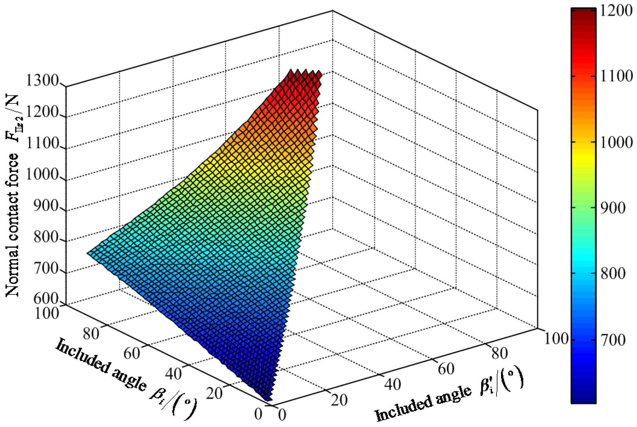
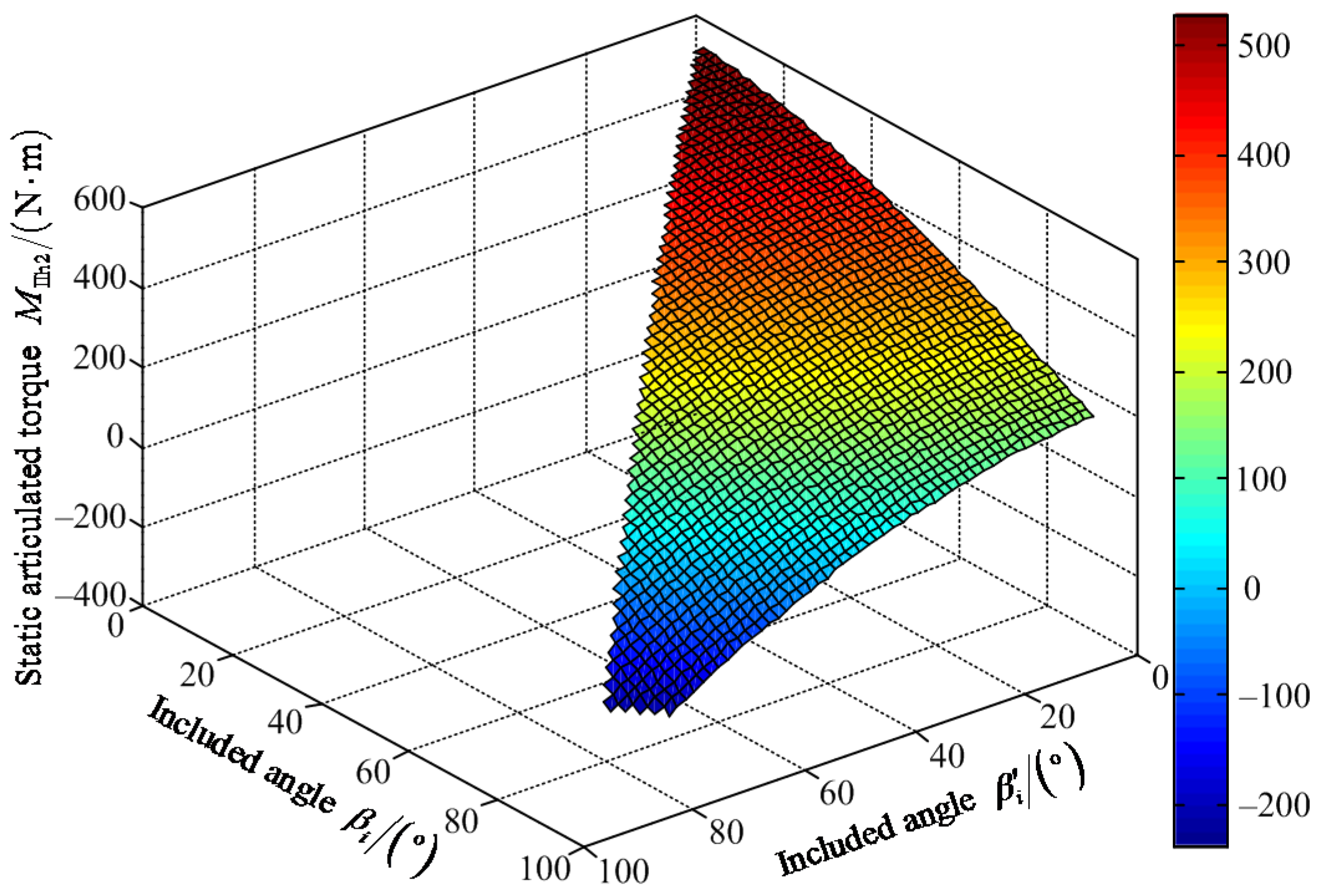
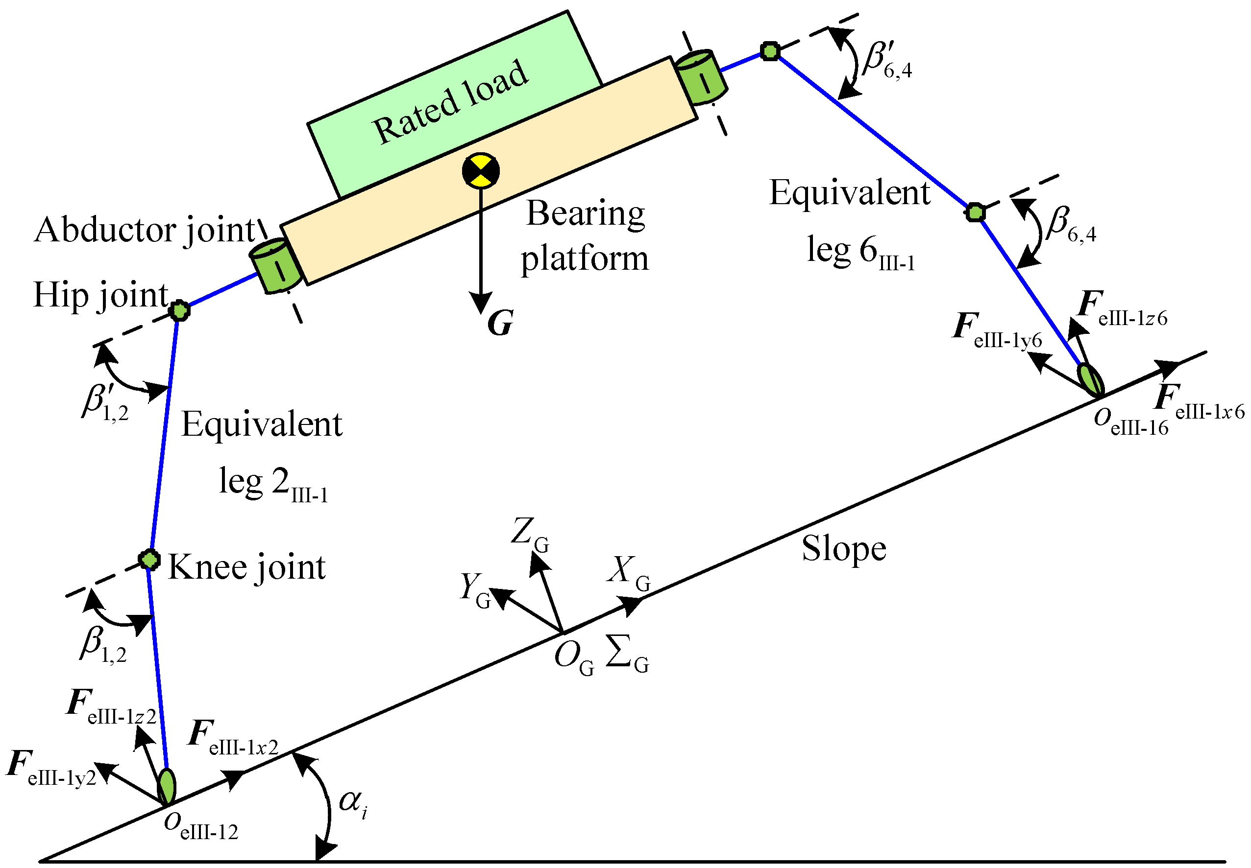
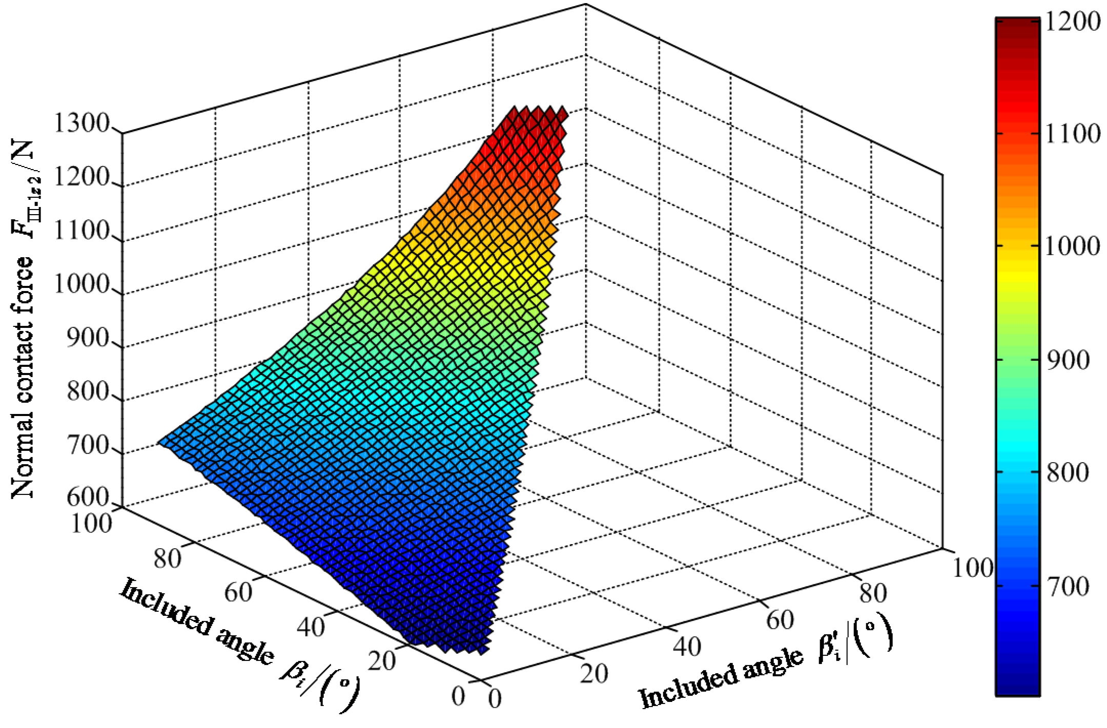
3.3.1. Analysis of Static Articulated Torques under Working Condition III-1

Based on Figure 6a, the static torques are solved for the hip joint and knee joint. The equivalent leg 6III-1 is obtained, when the equivalences are implemented through legs 4 and 6 to the straight line l1. The equivalent leg 2III-1 is obtained, when the equivalence is executed through leg 1 to leg 2. The equivalent model is shown in Figure 15. The moments of couples caused by the equivalence are ignored because their turnings are perpendicular to the tunings of torques of the hip joint and knee joint. They have no effect on solving the torques of the hip joint and knee joint. The relations of the included angles are obtained: β′1,2 = β′6,4 = β1′ = β2′ = β4′ = β6′ and β1,2 = β6,4 = β1 = β2 = β4 = β6.
According to Figure 6a and Figure 15, the inequalities can be obtained: FeIII-1z6FeIII-1z2 and FIII-1z1FeIII-1z2/2 ≤ FIII-1z2. Referring to the analysis of static articulated torques under working condition I, the normal contact force FeIII-1z2 of the equivalent leg 2III-1 can be solved. The mathematical expression is written for the static torque MIII-1h2 of hip joint and the static torque MIII-1k2 of knee joint of leg 2. Based on the constrained conditions of the working condition III-1: Gcos αi/4 ≤ FIII-1z2Gcos αi/2 and 0° ≤ βi′ ≤ βi ≤ 90°, the MATLAB software is selected to solve the normal contact force FIII-1z2, static torque MIII-1h2 of the hip joint, and static torque MIII-1k2 of the knee joint of leg 2. Their variable tendency charts with the changes of βi′ and βi are respectively shown in Figure 16, Figure 17 and Figure 18.
Figure 16 shows that the maximum value of FIII-1z2 is 1204.00 N when the values of included angles βi′ and βi are 78° and 89°, respectively. The minimum value of FIII-1z2 is 603.10 N when the value of included angle βi′ is zero and the value is 17° for the included angle βi. Figure 17 shows that the maximum value of positive static articulated torque MIII-1h2+ is 470.30 N·m when the values of included angles are 8° and 9° for βi′ and βi, respectively. The maximum value of negative static articulated torque MIII-1h2− is 243.90 N·m when the values of included angles βi′ and βi are 77° and 90°, respectively. Figure 18 shows that the maximum value of positive static articulated torque MIII-1k2+ is 252.20 N·m when the values are 9° for the included angles βi′ and βi. The maximum value of negative static articulated torque MIII-1k2− is 199.50 N·m when the value of included angle βi is 90° and the value of included angle βi′ can range from 0° to 77°. Thus, under the wording condition III-1 to climb the maximum slope, the included angle βi′ of the hip joint and the included angle βi of the knee joint should meet the conditions: 0° ≤ βi′ ≤ βi ≤ 90° and 17° ≤ βi′ + βi ≤ 167°.

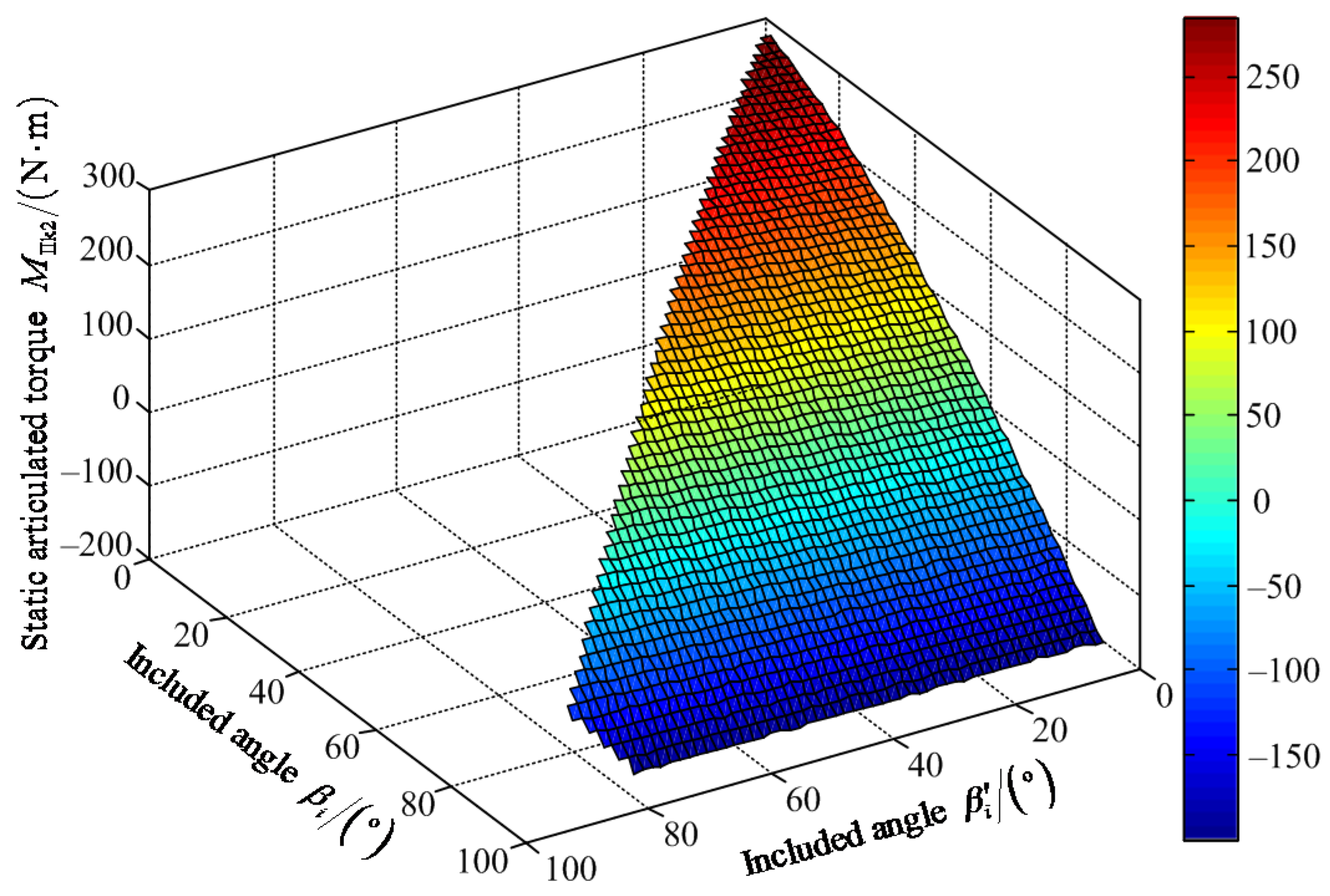
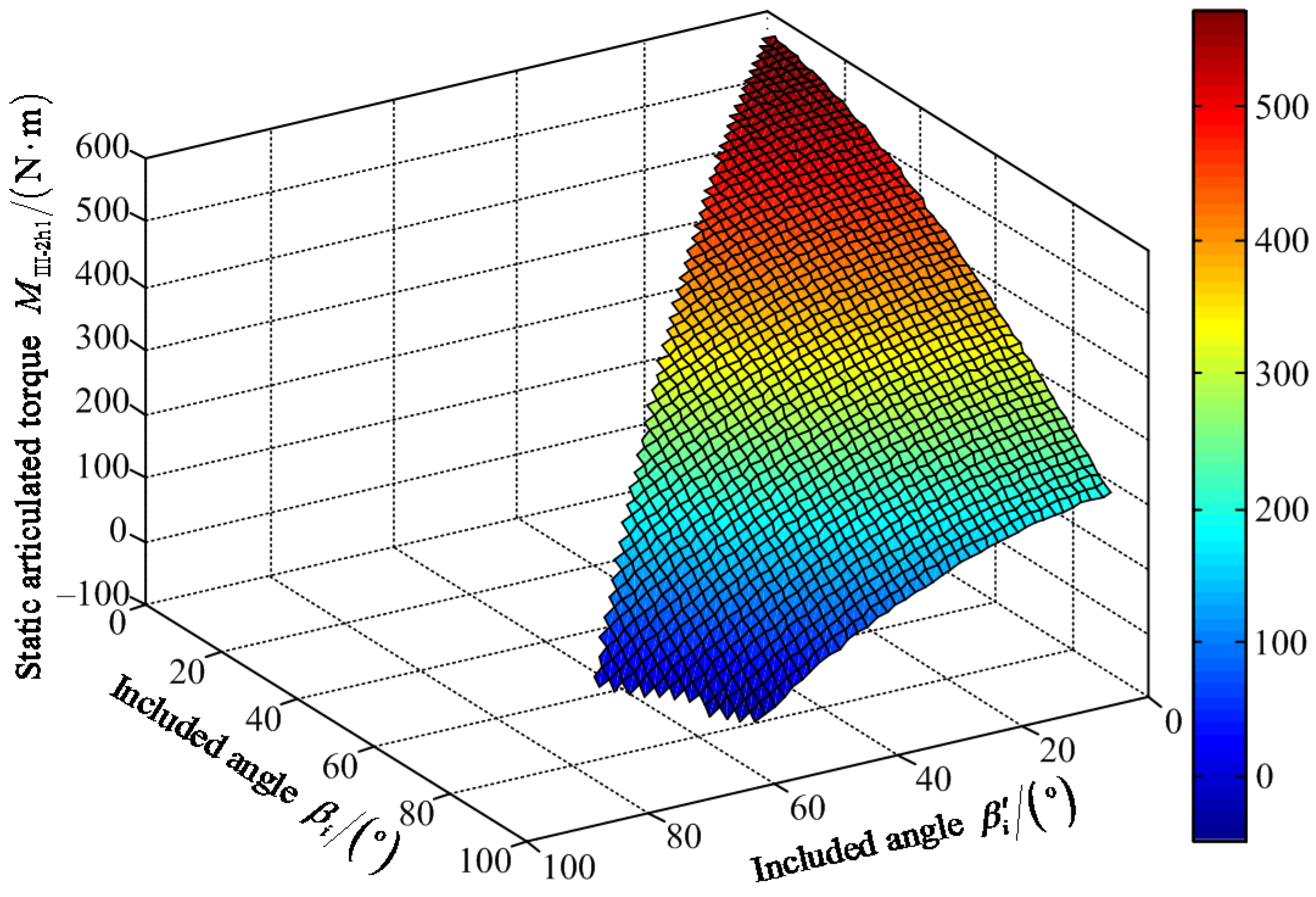
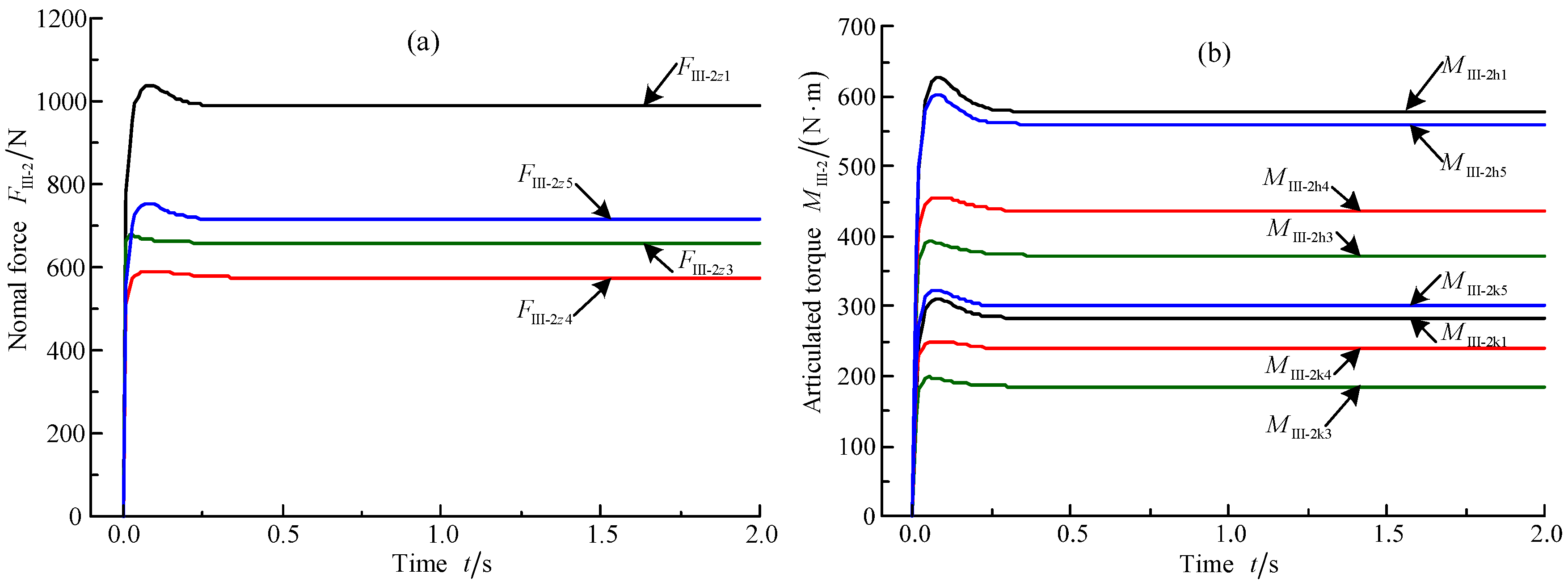
3.3.2. Analysis of Static Articulated Torques under Working Condition III-2

Based on Figure 6c, the static torques are solved for the hip joint and knee joint. The equivalent leg 1III-2 is obtained, when the equivalences are respectively executed through legs 1 and 3 to the straight line l1. The equivalent leg 5III-2 is acquired, when the equivalence is implemented through leg 4 to leg 5. The equivalent model is shown in Figure 19. The moments of couples that were brought by the equivalence can be ignored. The reason is that their turnings are perpendicular to the turnings of torques of the hip joint and knee joint. They have no effect on solving the static torques of the hip joint and knee joint. The relations of the included angles are acquired: β′1,3 = β′5,41′= β3′=β4′ = β5′ and β1,3 = β5,4 = β1 = β34 = β5.
Based on Figure 6c and Figure 19, the inequality is obtained: FeIII-2z5FeIII-2z1. Referring to the analysis of static articulated torques under working condition I, the normal contact force FeIII-2z1 can be solved. The mathematical expression can be written for the static torque MIII-2h1 of hip joint and static torque MIII-2k1 of knee joint of leg 1. According to the constrained condition of the working condition III-2: Gcos αi/4 ≤ FIII-2z1Gcos αi/2 and 0° ≤ βi′ ≤ βi ≤ 90°, the MATLAB software is used to solve the normal contact force FIII-2z1, static torque MIII-2h1 of the hip joint, and static torque MIII-2k1 of the knee joint of leg 1. Their variable tendency charts with the changes of βi′ and βi are, respectively, shown in Figure 20, Figure 21 and Figure 22.
Figure 20 shows that the maximum value of FIII-2z1 is 1204.00 N when the value of included angle βi′ is 62° and the value of included angle βi is 85°. The minimum value of FIII-2z1 is 642.80 N when the values of included angles βi′ and βi are zero. Figure 21 shows that the maximum value of positive static articulated torque MIII-2h1+ is 589.50 N·m when the values of included angles are zero for βi′ and βi. The maximum value of negative static articulated torque MIII-2h1− is 47.89 N·m when the values of included angles βi′ and βi are 57° and 90°, respectively. Figure 22 shows that the maximum value of positive static articulated torque MIII-2k1+ is 305.30 N·m when the values of included angles are zero for βi′ and βi. The maximum value of negative articulated torque MIII-2k1− is 199.50 N·m when the value of included angle βi is 90° and the value of included angle βi′ can range from 0° to 57°. According to Figure 20, Figure 21 and Figure 22, it can be concluded that the included angle βi′ of the hip joint and the included angle βi of the knee joint are limited. Under the wording condition III-2 to pass the maximum slope, the included angle βi′ of the hip joint and the included angle βi of the knee joint should meet the flowing requirements: 0° ≤ βi′ ≤ βi ≤ 90° and 0° ≤ βi′ + βi ≤ 147°.
According to the above research, the maximum static articulated torques of the hip joint and knee joint are respectively obtained. The relevant poses of the robot are also acquired when the crab-type quadrangular gait is employed to pass the maximum slope for the heavy-duty six-legged robot. The data of the maximum static articulated torques are shown in Table 2.
To increase the variety of gait for the heavy-duty six-legged robot, the maximum values of articulated torques in Table 2 are employed to select the driving devices and actuating devices for the hip joint and knee joint. Based on Table 2, it can be obtained that the maximum static torques of the hip joint and knee joint are, presented in the working condition III-2, 589.50 N·m and 305.30 N·m, respectively. The relevant poses of the robot are θi′ = βi′ = βi = 0°.

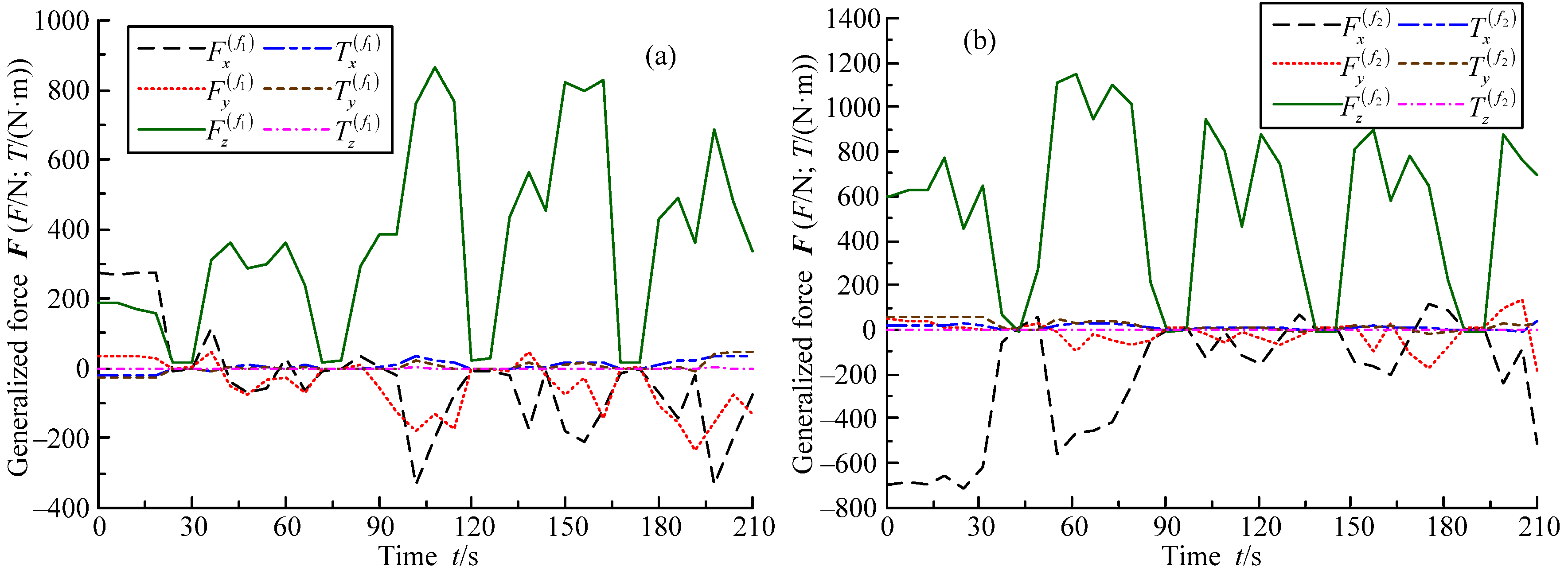
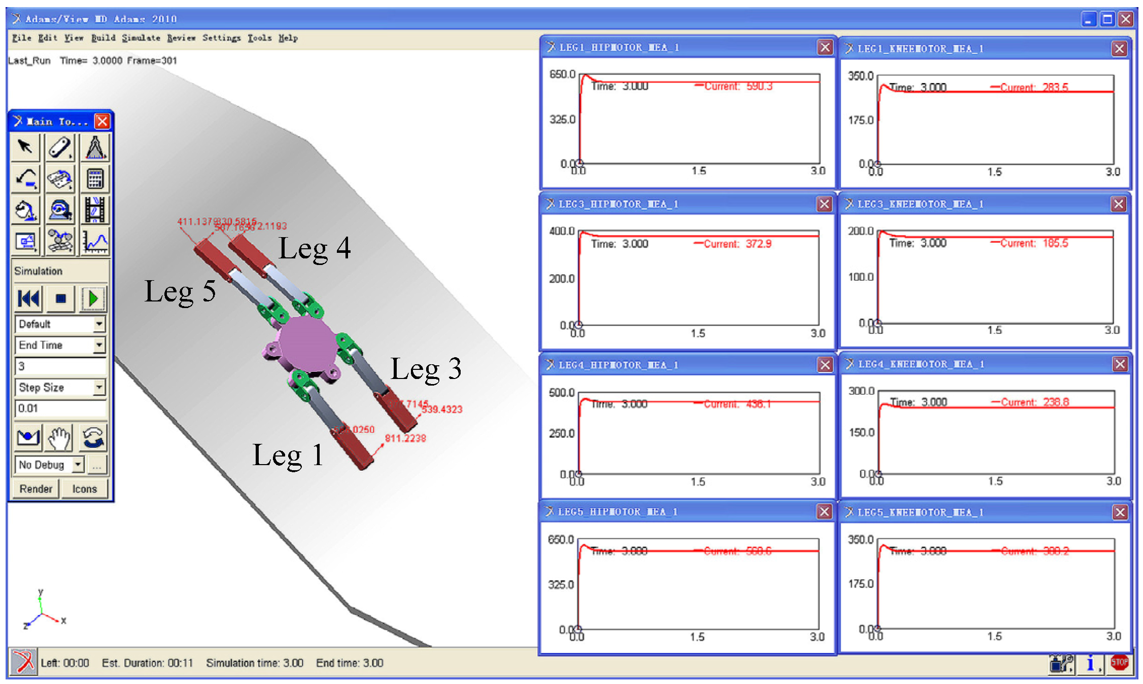
4. Simulation Analysis

Due to the same analysis method of the articulated torques under the working conditions I, II, and III, the maximum articulated torque in Table 2 is only performed for the simulation verification. Based on Table 2, it can be obtained that the hip joint and knee joint have the maximum articulated torques when the crab-type quadrangular gait is employed to pass the maximum slope in the working condition III-2, and the robot poses are θi′ = βi′ = βi = 0°. Actually, the values of included angles βi′ and βi are not zero because the underside of the bearing platform cannot contact the ground. Based on the structure of the robot, the underside of the bearing platform dangerously contacts the ground when the values are 2° for the included angles βi′ and βi.
The structures of the shins have been simplified, but the positions of the mass centers and effective lengths are not changed. Thus, the simulation results of the articulated torques are reliable. Based on the assumed parameters and the robot poses which are θi′ = 0° and βi′ = βi = 2°, the SolidWorks software (SolidWorks 2010, Dassault Systemes S.A., Concord, MA, USA) is used to construct 3-D model of the support phase under the working condition III-2. Furthermore, 3-D model is imported the ADAMS software (ADAMS 2010, Mechanical Dynamics Inc., Los Angeles, CA, USA) to carry out the simulation, as shown in Figure 23. The mass of the transfer phase that has been ignored is added up to the gravity center of the bearing platform. Then, the static simulation is performed for the articulated torques of the support phase, and the simulation curves are obtained for the normal contact forces, torques of the hip joints, and torques of the knee joints, respectively, as shown in Figure 24.
Based on Figure 24, it can be concluded that the normal contact forces, static torques of the hip joints, and static torques of the knee joints all instantaneously increase from the value of 0 to the maximum peak value, and then reduce from the maximum peak value to the constant value in a short time. The tendencies of curves of the normal contact force and articulated torques basically keep consistent with the practical situation of the heavy-duty six-legged robot.
According to Figure 24a, the relations of the normal contact forces in the support phase can be obtained: FIII-2z4 < FIII-2z3 < FIII-2z5 < FIII-2z1. The reason can be illustrated as follows. Based on Figure 6c, leg 1 locates the left side of the mass center of the bearing platform, and legs 3 and 4 lie in the right side of the mass center of the bearing platform, which results in a larger normal contact force on the foothold of leg 1. According to Figure 24a and the research results of Section 3, it can be obtained that the theoretical analysis value, 1204.00 N, is bigger than the simulation value, 1038.44 N, for the normal contact force of leg 1.
Based on Figure 24b, the relations of the static torques of the hip joints can be obtained: MIII-2h3 < MIII-2h4 < MIII-2h5 < MIII-2h1. Meanwhile, the maximum simulation value of static torque is 620.01 N·m for the hip joint of leg 1. That is about 1.05 times its theoretical calculation value. The value of analytical error is about 5%. According to Figure 24b, the relations of static torques of the knee joints can be also acquired: MIII-2k3 < MIII-2k4 < MIII-2k1 < MIII-2k5. Meanwhile, the maximum simulation value of static torque is 311.03 N·m for the knee joint of leg 1. That is about 1.02 times its theoretical calculation value. The value of analytical error is about 2%. Although leg 5 has the maximum torque of the knee joint in the simulation, and its value is 315.01 N·m, the value is only 1.03 times the theoretical calculation value of the torque of knee joint of leg 1. The analytical error is small, only 3%.
On the whole, the theoretical calculation values basically keep consistent with the simulation values on solving the static articulated torques. That verifies the reasonableness of the theoretical analysis on the torques of the hip joint and knee joint. The availability of the static simulation of the ADAMS software is simultaneously validated on analyzing the torques of joints.

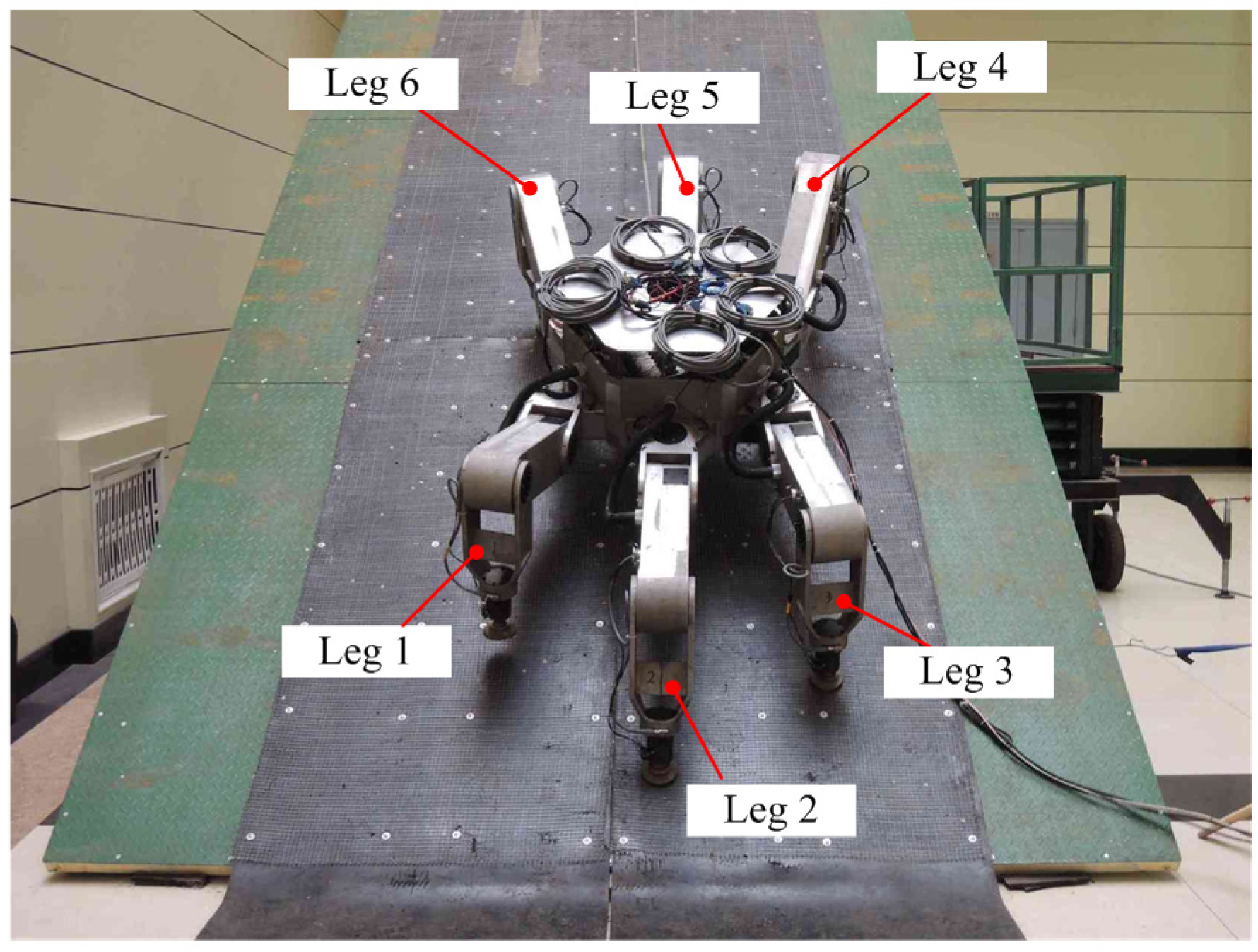
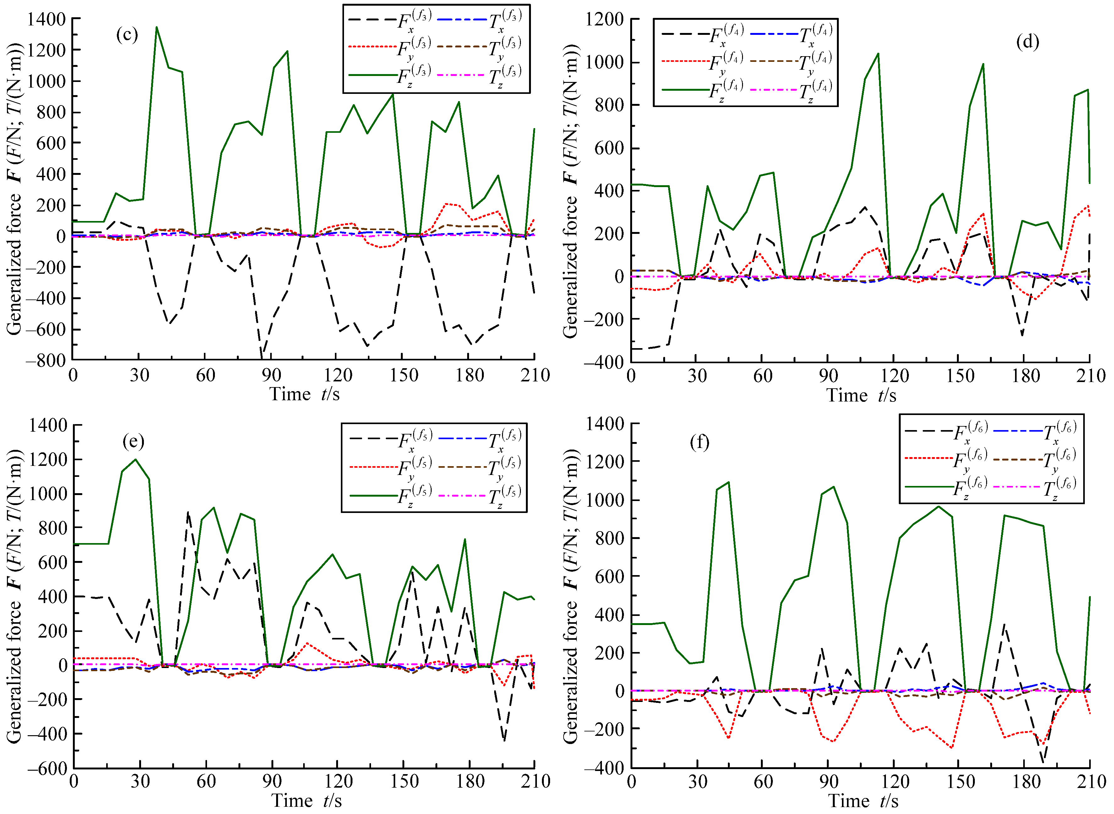
5. Applications and Experiments

Based on the analysis method of the static articulated torques in this article and the real data parameters of robot, the prototype of electrically driven heavy-duty six-legged robot is developed. Its climbing experiments are executed, as shown in Figure 25. The maximum walking speed of the prototype is only 0.1 m/s on the flat terrain, which is slow. Thus, it can be considered that the walking speed has no influence on the analysis of the articulated torques when the robot climbs the maximum slope under the low walking speed. The walking experiments of the robot can be employed to check whether the theoretical analysis and simulation of static articulate torque are available or not. If the prototype of electrically driven heavy-duty six-legged robot can successfully traverse the maximum slope, the analysis method of articulated torque in this article can be viewed as reasonable. This method is suitable for analyzing articulated torque when the heavy-duty six-legged robot walks by the quadrangular gait.
When the crab-type quadrangular gait is employed to pass the maximum slope for the heavy-duty six-legged robot, the distance is 350 mm from the underside of the bearing platform to the slope. The swing sequences of legs in one period are legs 3 and 6 in the 1/3 gait, legs 1 and 4 in the 2/3 gait, and legs 2 and 5 in the last 1/3 gait. Due to the large mass of the heavy-duty six-legged robot, it is necessary to increase the stability of robot when it passes the maximum slope. Thus, the initial rotation angles of the abductor joints are set as 10° for legs 1, 3, 4 and 6.
Although the data of the articulated torques are not collected because there are no torque sensors in the robot, the generalized forces of feet can be discretely collected by the six-dimension force sensors of the feet. The generalized force curves are shown in Figure 26. To keep the real data of the generalized forces, the generalized force curves are not smoothed. In Figure 26, the generalized force curves exhibit little perturbations. Two main reasons can be illustrated as follows. First, the rubber slabs and steel meshes are installed on the slope for enhancing the adhesion forces of the robot’s feet. They produce little deformation when the robot walks. Second, the quadrangular gait leads to the statically indeterminate problem. One leg may bear the small or big normal contact force in the short or long time. Although the generalized force curves present partial perturbations, they still have the much higher value in use.
The feet of legs 1, 3, 4 and 6 undertake the y-direction forces due to their abductor joints of 10°. Although the y-direction forces lead to the torques of abductor joints, the values of articulated torques are smaller. The torques of the hip joints and knee joints can be estimated based on the generalized force curves of feet and corresponding poses of the robot. Then, it is found that the values of articulated torques are in the allowable range. Based on Figure 26, it can be concluded that the torques of feet are much small in the directions x and y and approximate zero in the direction z. This conclusion is consistent with the actual working conditions.
In addition, when the crab-type quadrangular gait is used to transit the maximum slope for the heavy-duty six-legged robot, it is found that the all joints can work normally. The braking phenomenon does not occur because the driving devices and actuating devices cannot provide the enough output torques. The robot can independently overpass the maximum slope. Therefore, the results of experiments can prove that the analysis method of the articulated torque is reasonable in this article.

6. Conclusions

In this article, the analysis method of the articulated torque is presented under the quadrangular gait. The highly stable swing sequences of legs are acquired. Based on the crab-type quadrangular gait, the typical working conditions are analyzed in the support phase. The maximum normal contact forces and static articulated torques are solved when the robot transits the maximum slope. Meanwhile, the relevant poses of the robot are also obtained.
Based on the pose of robot under the maximum static articulated torque, the static simulation is executed. The simulation values are obtained, including the normal contact forces and the articulated torques. Through the comparative analysis of the maximum static articulated torques, it shows that the theoretical calculation values are smaller than the simulation values. The maximum error appears in the hip joint, whose value is about 5%. Based on the analysis method of the articulated torque in this article, a prototype of electrically driven heavy-duty six-legged robot is developed. The climbing experiments of the prototype proved that the analysis method of the articulated torques is reasonable. The proposed method can be applied to solve the static torques of joints of the robot.

Acknowledgments

This work was supported by the National Natural Science Foundation of China (Grant No. 51505335 and Grant No. 51275106).

Author Contributions

Hong-Chao Zhuang conceived the topic, developed the equations, and implemented the simulation analysis; Hong-Chao Zhuang, Hai-Bo Gao and Zong-Quan Deng performed the applications and experiments; and Hong-Chao Zhuang wrote the paper.

Conflicts of Interest

The authors declare no conflict of interest.

References

  1. Wang, D.L.; Leung, H.; Kurian, A.P.; Kim, H.-J.; Yoon, H. A deconvolutive neural network for speech classification with applications to home service robot. IEEE Trans. Instrum. Meas. 2010, 59, 3237–3243. [Google Scholar] [CrossRef]
  2. Krotkov, E.P.; Simmons, R.G.; Whittaker, W.L. Ambler: Performance of a six-legged planetary rover. Acta Astronaut. 1995, 35, 75–81. [Google Scholar] [CrossRef]
  3. Wilcox, B.H.; Litwin, T.; Biesiadecki, J.; Matthews, J.; Heverly, M.; Morrison, J.; Townsend, J.; Ahmad, N.; Sirota, A.; Cooper, B. ATHLETE: A cargo handling and manipulation robot for the moon. J. Field Robot. 2007, 24, 421–434. [Google Scholar] [CrossRef]
  4. Luk, B.L.; Cooke, D.S.; Galt, S.; Collie, A.A.; Chen, S. Intelligent legged climbing service robot for remote maintenance applications in hazardous environments. Robot. Auton. Syst. 2005, 53, 142–152. [Google Scholar] [CrossRef]
  5. Irawan, A.; Nonami, K. Compliant walking control for hydraulic driven hexapod robot on rough terrain. J. Robot. Mechatron. 2011, 23, 149–162. [Google Scholar]
  6. Roy, S.S.; Pratihar, D.K. Effects of turning gait parameters on energy consumption and stability of a six-legged walking robot. Robot. Auton. Syst. 2012, 60, 72–82. [Google Scholar] [CrossRef]
  7. Hyon, S.H.; Emura, T. Energy-preserving control of a passive one-legged running robot. Adv. Robot. 2004, 18, 357–381. [Google Scholar] [CrossRef]
  8. Raibert, M.; Blankespoor, K.; Nelson, G.; Playter, R.; the BigDog Team. BigDog, the rough-terrain quadruped robot. In Proceedings of the 17th World Congress, International Federation of Automatic Control, Seoul, Korea, 6–11 July 2008.
  9. Silva, M.F.; Machado, J.A.T. A historical perspective of legged robots. J. Vib. Control 2007, 13, 1447–1486. [Google Scholar] [CrossRef]
  10. Liu, J.; Tan, M.; Zhao, X.G. Legged robots—An overview. Trans. Inst. Meas. Control 2007, 29, 185–202. [Google Scholar] [CrossRef]
  11. Erden, M.S.; Leblebicioğlu, K. Free gait generation with reinforcement learning for a six-legged robot. Robot. Auton. Syst. 2008, 56, 199–212. [Google Scholar] [CrossRef]
  12. Kurashige, K.; Fukuda, T.; Hoshino, H. Reusing primitive and acquired motion knowledge for gait generation of a six-legged robot using genetic programming. J. Intell. Robot. Syst. 2003, 38, 121–134. [Google Scholar] [CrossRef]
  13. Zhang, X.L.; E, M.C.; Zeng, X.Y.; Zheng, H.J. Adaptive walking of a quadrupedal robot based on layered biological reflexes. Chin. J. Mech. Eng. 2012, 25, 654–664. [Google Scholar] [CrossRef]
  14. Irawan, A.; Nonami, K. Optimal impedance control based on body inertia for a hydraulically driven hexapod robot walking on uneven and extremely soft terrain. J. Field Robot. 2011, 28, 690–713. [Google Scholar] [CrossRef]
  15. Luk, B.L.; Galt, S.; Chen, S. Using genetic algorithms to establish efficient walking gaits for an eight legged robot. Int. J. Syst. Sci. 2001, 32, 703–713. [Google Scholar] [CrossRef]
  16. Tan, G.Z.; He, H.; Sloman, A. Global optimal path planning for mobile robot based on improved Dijkstra algorithm and ant system algorithm. J. Cent. South Univ. Technol. 2006, 13, 80–86. [Google Scholar] [CrossRef]
  17. Sintov, A.; Avramovich, T.; Shapiro, A. Design and motion planning of an autonomous climbing robot with claws. Robot. Auton. Syst. 2011, 59, 1008–1019. [Google Scholar] [CrossRef]
  18. Erden, M.S.; Leblebicioğlu, K. Torque distribution in a six-legged robot. IEEE Trans. Robot. 2007, 23, 179–186. [Google Scholar] [CrossRef]
  19. Roy, S.S.; Singh, A.K.; Pratihar, D.K. Estimation of optimal feet forces and joint torques for on-line control of six-legged robot. Robot. Comput. Integr. Manuf. 2011, 27, 910–917. [Google Scholar] [CrossRef]
  20. Santos, P.G.D.; Estremera, J.; Garcia, E.; Armada, M. Including joint torques and power consumption in the stability margin of walking robots. Auton. Robot. 2005, 18, 43–57. [Google Scholar] [CrossRef]
  21. Silva, M.F.; Machado, J.A.T.; Lopes, A.M. Fractional order control of a hexapod robot. Nonlinear Dyn. 2004, 38, 417–433. [Google Scholar] [CrossRef]
  22. Mahapatra, A.; Roy, S.S. Computer aided dynamic simulation of six-legged robot. Int. J. Recent Trends Eng. 2009, 2, 146–151. [Google Scholar]
  23. Wang, G.; Zhang, L.X.; Chen, D.L.; Liu, D.F.; Chen, X. Modeling and simulation of multi-legged walking machine prototype. In Proceedings of the 2009 International Conference on Measuring Technology and Mechatronics Automation, Zhangjiajie, China, 11–12 April 2009.
  24. Gao, H.B.; Zhuang, H.C.; Deng, Z.Q.; Ding, L.; Liu, Z. Transmission mode research on the joints of a multi-legged walking robot. Appl. Mech. Mater. 2012, 151, 518–522. [Google Scholar] [CrossRef]
  25. Gao, H.B.; Zhuang, H.C.; Li, Z.G.; Deng, Z.Q.; Ding, L.; Liu, Z. Optimization and experimental research on a new-type short cylindrical cup-shaped harmonic reducer. J. Cent. South Univ. Technol. 2012, 19, 1869–1882. [Google Scholar] [CrossRef]
  26. Zhuang, H.C.; Gao, H.B.; Deng, Z.Q.; Ding, L.; Liu, Z. Method for analyzing articulated rotating speeds of heavy-duty six-legged robot. J. Mech. Eng. 2013, 49, 44–52. [Google Scholar] [CrossRef]
  27. Zhuang, H.C.; Gao, H.B.; Deng, Z.Q.; Ding, L.; Liu, Z. A review of heavy-duty legged robots. Sci. China Technol. Sci. 2014, 57, 298–314. [Google Scholar] [CrossRef]
Figure 1. Electrically driven heavy-duty six-legged robot: (a) mechanism; and (b) structure of leg.
Applsci 06 00323 g001
Figure 2. Four kinds of typical walking ways of heavy-duty six-legged robot under quadrangular gait: (a) crab type; (b) crab–ant mixed type I; (c) ant type; and (d) crab–ant mixed type II.
Applsci 06 00323 g002
Figure 3. Simplified 3-D model of robot using crab-type quadrangular gait to pass slope.
Applsci 06 00323 g003
Figure 4. Working condition I of support phase: (a) support phase involving legs 1, 3, 4 and 6; and (b) equivalent support phase of legs 1, 3, 4 and 6.
Applsci 06 00323 g004
Figure 5. Working condition II of support phase: (a) support phase involving legs 1, 2, 4 and 5; and (b) support phase involving legs 2, 3, 5 and 6.
Applsci 06 00323 g005
Figure 6. Working condition III of support phase: (a) support phase involving legs 1, 2, 4 and 6; (b) support phase involving legs 2, 3, 4 and 6; (c) support phase involving legs 1, 3, 4 and 5; and (d) support phase involving legs 1, 3, 5 and 6.
Applsci 06 00323 g006
Figure 7. Equivalent model of support phase under working condition I.
Applsci 06 00323 g007
Figure 8. Variable tendency chart of normal contact force FIz1 with changes of βi′ and βi.
Applsci 06 00323 g008
Figure 9. Variable tendency chart of static articulated torque MIh1 with changes of βi′ and βi.
Applsci 06 00323 g009
Figure 10. Variable tendency chart of static articulated torque MIk1 with changes of βi′ and βi.
Applsci 06 00323 g010
Figure 11. Equivalent model of support phase under working condition II.
Applsci 06 00323 g011
Figure 12. Variable tendency chart of normal contact force FIIz2 with the changes of βi′ and βi.
Applsci 06 00323 g012
Figure 13. Variable tendency chart of static articulated torque MIIh2 with changes of βi′ and βi.
Applsci 06 00323 g013
Figure 14. Variable tendency chart of static articulated torque MIIk2 with changes of βi′ and βi.
Applsci 06 00323 g014
Figure 15. Equivalent model of support phase under working condition III-1.
Applsci 06 00323 g015
Figure 16. Variable tendency chart of normal contact force FIII-1z2 with the changes of βi′ and βi.
Applsci 06 00323 g016
Figure 17. Variable tendency chart of static articulated torque MIII-1h2 with changes of βi′ and βi.
Applsci 06 00323 g017
Figure 18. Variable tendency chart of static articulated torque MIII-1k2 with changes of βi′ and βi.
Applsci 06 00323 g018
Figure 19. Equivalent model of support phase under working condition III-2.
Applsci 06 00323 g019
Figure 20. Variable tendency chart of normal contact force FIII-2z1 with the changes of βi′ and βi.
Applsci 06 00323 g020
Figure 21. Variable tendency chart of static articulated torque MIII-2h1 with changes of βi′ and βi.
Applsci 06 00323 g021
Figure 22. Variable tendency chart of static articulated torque MIII-2k1 with changes of βi′ and βi.
Applsci 06 00323 g022
Figure 23. Simulation of static articulated torque of support phase under working condition III-2.
Applsci 06 00323 g023
Figure 24. Simulation curves: (a) normal forces of support phase; and (b) static torques of hip joints and knee joints in support phase.
Applsci 06 00323 g024
Figure 25. Climbing maximum slope experiments of robot under crab-type quadrangular gait.
Applsci 06 00323 g025
Figure 26. Generalized force curves of feet: (a) leg 1; (b) leg 2; (c) leg 3; (d) leg 4; (e) leg 5; and (f) leg 6.
Applsci 06 00323 g026aApplsci 06 00323 g026b
Table 1. Higher-stable swing sequences of legs under quadrangular gait.
No.Phase1/3 Gait Legs2/3 Gait Legs3/3 Gait LegsNo.Phase1/3 Gait Legs2/3 Gait Legs3/3 Gait Legs
1Transfer1, 52, 43, 610Transfer2, 53, 61, 4
Support2, 3, 4, 61, 3, 5, 61, 2, 4, 5Support1, 3, 4, 61, 2, 4, 52, 3, 5, 6
2Transfer1, 53, 62, 411Transfer2, 43, 61, 5
Support2, 3, 4, 61, 2, 4, 51, 3, 5, 6Support1, 3, 5, 61, 2, 4, 52, 3, 4, 6
3Transfer1, 42, 53, 612Transfer2, 41, 53, 6
Support2, 3, 5, 61, 3, 4, 61, 2, 4, 5Support1, 3, 5, 62, 3, 4, 61, 2, 4, 5
4Transfer1, 42, 63, 513Transfer3, 62, 51, 4
Support2, 3, 5, 61, 3, 4, 51, 2, 4, 6Support1, 2, 4, 51, 3, 4, 62, 3, 5, 6
5Transfer1, 43, 62, 514Transfer3, 62, 41, 5
Support2, 3, 5, 61, 2, 4, 51, 3, 4, 6Support1, 2, 4, 51, 3, 5, 62, 3, 4, 6
6Transfer1, 43, 52, 615Transfer3, 61, 52, 4
Support2, 3, 5, 61, 2, 4, 61, 3, 4, 5Support1, 2, 4, 52, 3, 4, 61, 3, 5, 6
7Transfer2, 63, 51, 416Transfer3, 61, 42, 5
Support1, 3, 4, 51, 2, 4, 62, 3, 5, 6Support1, 2, 4, 52, 3, 5, 61, 3, 4, 6
8Transfer2, 61, 43, 517Transfer3, 51, 42, 6
Support1, 3, 4, 52, 3, 5, 61, 2, 4, 6Support1, 2, 4, 62, 3, 5, 61, 3, 4, 5
9Transfer2, 51, 43, 618Transfer3, 52, 61, 4
Support1, 3, 4, 62, 3, 5, 61, 2, 4, 5Support1, 2, 4, 61, 3, 4, 52, 3, 5, 6
Table 2. Maximum static torques of hip joint and knee joint.
No.Max. Static Torque of Hip JointMax. Static Torque of Knee JointRange
PoseValue/N·mPoseValue/N·m
Iβi′ = 0°529.80βi′ = 0°285.000° ≤ βi′ ≤ βi ≤ 90°
βi = 0°βi = 0°0° ≤ βi′ + βi ≤ 147°
IIβi′ = 0°529.80βi′ = 0°285.000° ≤ βi′ ≤ βi ≤ 90°
βi = 0°βi = 0°0° ≤ βi′ + βi ≤ 167°
III-1βi′ = 8°470.30βi′ = 9°252.200° ≤ βi′ ≤ βi ≤ 90°
βi = 9°βi = 9°17° ≤ βi′ + βi ≤ 167°
III-2βi′ = 0°589.50βi′ = 0°305.300° ≤ βi′ ≤ βi ≤ 90°
βi = 0°βi = 0°0° ≤ βi′ + βi ≤ 147°

