1. Introduction
Modern energy demands have prompted the United States Bureau of Land Management (BLM) to develop utility-scale solar energy installations and transmission infrastructure in parts of southern California’s Mojave and Lower Colorado Deserts. The BLM and Department of Energy’s Programmatic Environmental Impact Statement (PEIS) for Solar Energy Development in Six Southwestern States (2012) and the BLM Desert Renewable Energy Conservation Plan (DRECP) (2016) have shaped the design of solar development in southeast California. The DRECP covers parts of seven California counties: Imperial, Inyo, Kern, Los Angeles, Riverside, San Bernardino, and San Diego. Approximately 91,000 km
2 of federal and nonfederal California desert land are part of the DRECP area. A key objective of the DRECP is to “provide effective protection and conservation of desert ecosystems while allowing for the appropriate development of renewable energy projects” [
1]. On BLM public lands in California, solar energy zones (SEZs) established through the PEIS and Development Focus Areas (DFAs) for DRECP solar energy development provide a mechanism to facilitate installation of renewable energy production sites.
Vegetation cover change from renewable energy development is receiving increasing attention due to potential impacts on protected area conservation, endangered species, and air quality [
2]. The objective of the study is to assess the influence of solar energy development sites in parts of the Mojave and Sonoran Deserts on changes to vegetation indices (VIs), and to develop a reproducible framework for detection of variable ecological change. Abrupt changes, or “breakpoints,” in vegetation cover may adversely affect habitats for wildlife, which may not adapt sufficiently quickly to new conditions. These impacts would then disrupt both the primary and secondary productivity of the desert ecosystem. Change detection using remotely sensed data offers an opportunity for federal, state, and local agencies to jointly monitor and respond to major changes in ecological conditions that might occur in and near solar facilities.
Numerous published studies [
3,
4,
5,
6,
7,
8,
9] have reported the close correlation between the normalized difference vegetation index (NDVI) from satellite sensors and measurements of percent cover of green vegetation canopies in arid ecosystems. More specifically, Ramsey et al. [
10] found that NDVI from Landsat was tightly correlated (
r = 0.88;
p < 0.05) with total percent cover of live vegetation in a semi-arid sagebrush ecosystem in south-central Utah. Potter [
2] reported that interannual variations in precipitation accounted for nearly all the periodic changes in Landsat NDVI in shrubland communities observed since 1985 across the Lower Colorado Desert of California.
The focus of this study is on the influence of the construction and operation of solar energy facilities on the past and present natural vegetation cover, as expressed in MODIS VIs (for live green vegetation density). For this research, we use a 19-year vegetation index (VI) time series from Collection 6 of the Terra Moderate Resolution Imaging Spectroradiometer (MODIS) satellite with the Breaks for Additive Season and Trend (BFAST) method to detect significant changes in vegetation cover in southern California deserts. First, we evaluated the suitability of three VIs for use with the BFAST model in the study area and determine the best suited VI. Next, we examined change detection time series results at several solar energy sites to infer any vegetation response patterns. Finally, we analyzed distributional statistics for breakpoints to characterize more general responses at each study area.
Our results will help to locate regions sensitive to disturbances and, in turn, inform future policy decisions. Furthermore, this methodology is fully extensible to incorporate newly released MODIS observations because aggregation of observations minimizes issues like cloud cover and thus ensures a consistent regularly-spaced VI time series. This fact enhances the utility of the method to long-term monitoring efforts, as required by the BLM.
2. Study Area
In our study area, the Mojave Desert is transitional between the lower, hotter Lower Colorado Desert to the south and the colder high desert of the Great Basin to the north [
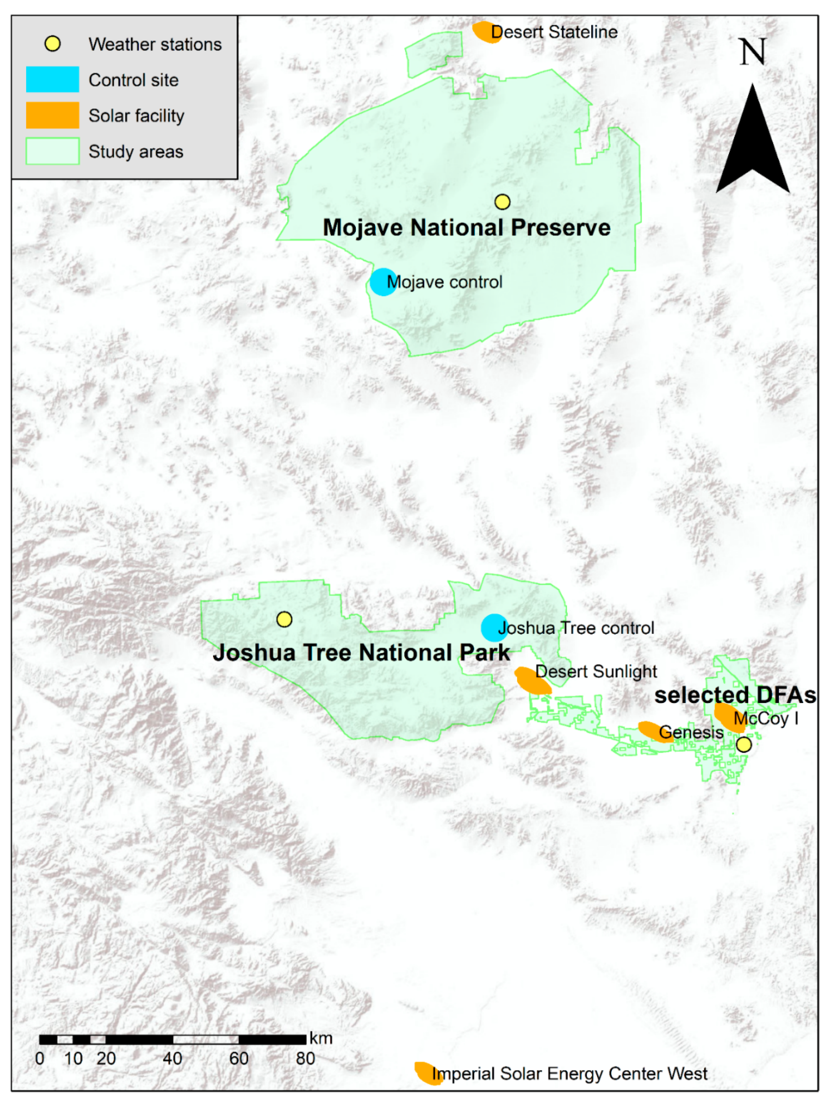
1]. The first set of study sites was comprised five solar energy facilities (Genesis, Imperial Solar Energy Center West, McCoy, Desert Sunlight, and Desert Stateline), constituting the analysis at the finer spatial scale (
Figure 1). At the larger regional scale, the main areas of interest for this study were Joshua Tree National Park (JOTR), Mojave National Preserve and Wilderness (MOJA), and a proximal group of solar energy DFAs in Imperial, Riverside, and San Bernardino counties, California (
Figure 1) on BLM lands. NPS sites provide controls as more protected and undisturbed landscapes.
The main perennial vegetation cover type in the study area is creosote bush (
Larrea divaricata) and white bursage (
Ambrosia dumosa) [
1,
2], although ironwood (
Olneya tesota), palo verde (
Cercidium floridum), Joshua tree (
Yucca brevifolia), and ocotillo (
Fouquieria splendens) are also found throughout the region. Low annual rainfall (50–300 mm) and high temperatures (exceeding 45 °C in the summer) make this area one of the most arid in North America [
1].
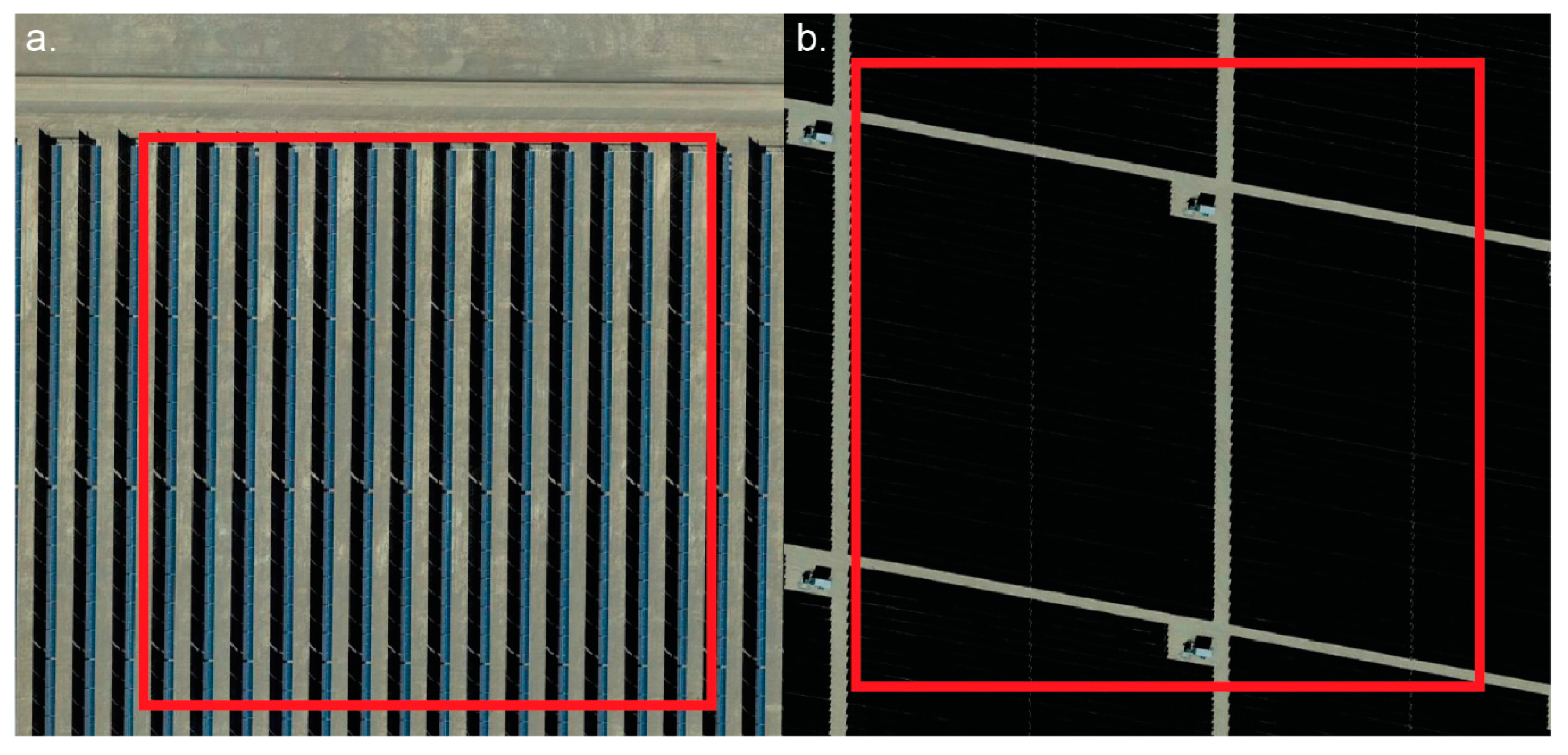
The five solar energy facilities examined here featured two general spatial patterns of solar arrays. The first pattern is characterized by rows/columns of solar installations with wider spacing (
Figure 2a), and was apparent at three sites (Genesis, McCoy, Imperial). The second pattern is characterized by tighter spacing in between blocks of arrays (
Figure 2b), and was exhibited at two sites (Desert Sunlight, Desert Stateline).
3. Methods
The conceptual framework of the method follows a broad sequence of (1) processing, (2) selection, and (3) analysis. The inputs to the processing stage are the data for the proposed VIs (EVI, NDVI, and SAVI). Each spatiotemporal VI dataset is first preprocessed for data quality. Then, BFAST time series analysis results are produced for each preprocessed VI dataset.
The goal of the selection phase is to choose the most suitable VI for the final analysis phase. Here, “suitability” is taken to be the strength of the response to known vegetation influences (precipitation and wildfire). The preprocessed VI dataset and BFAST results are jointly used for this determination.
The final stage, analysis, uses the BFAST result from the selected VI in the previous phase to perform statistical analysis at two spatial scales, at the scale of solar energy facilities and the regional scale. Thus, two statistical techniques, spatial kernel density estimation and bootstrapping, are adopted to address the varying analysis scales. The key outputs of this method, then, are the spatiotemporal BFAST results and the statistical analyses, which summarize the BFAST results within discrete units of the study area at two spatial scales. The details follow in the remainder of this section.
3.1. Processing Phase: Vegetation Index Selection
The VIs considered in this study were the normalized difference vegetation index (NDVI), enhanced vegetation index (EVI), and the soil-adjusted vegetation index (SAVI). NDVI was selected because of its simplicity and ease of interpretation, while EVI and SAVI were selected as alternatives that tend to reduce the interference of the canopy background signal [
11,
12]. In addition, these VIs were chosen because of their prevalence and extensive documentation in the scientific literature [
11,
12]. These VIs are calculated as a function of the reflectance in different spectral bands (
Table 1). Each VI ranges from −1 to 1, with higher values indicating more greenness and denser vegetation.
3.2. Processing Phase: Satellite Imagery
Time series for NDVI, EVI, and SAVI are derived from Collection 6 vegetation index 16-day aggregate raster grids (MOD13Q1) from the Terra MODIS sensor at 250-m resolution [
14]. The satellite observations range from February 2000 to May 2018 at 16-day intervals, having been composited from daily data. Terra MODIS data were chosen for this study because of the relatively higher number of observations for a given time period, which avoids most atmospheric issues, and reasonable spatial resolution. In contrast, Landsat data have a much finer spatial resolution but its comparatively lower number of observations for a given time, and thus higher risk of atmospheric contamination, make it less reliable for time series analysis in which consistent and regularly-spaced data points are necessary.
The VI datasets were obtained using the “MODIStsp” R package [
15] to automate creation of time-series rasters from MODIS data. NDVI and EVI data are directly available as prepackaged products, but SAVI must be computed from the MODIS spectral band reflectances. Any pixel observations with cloud, snow, or ice cover were eliminated from each dataset according to pixel reliability values [
16].
Each VI dataset was reaggregated to monthly observations based on the maximum VI value in a given month. Reaggregation was necessary to reduce processing time for subsequent steps. The maximum VI values served as the reaggregation statistic to further reduce any chance of atmospheric contamination, which would tend to decrease the VI reading. Any remaining missing data were interpolated linearly only if the time series did not have greater than 5% missing data or did not have four or more consecutive missing data points. The final result was a raster dataset for VI values for monthly observations from February 2000 to May 2018 for a total of 220 observations.
3.3. Processing Phase: Time Series Change Detection
In order to quantify the significance of fluctuations in the VI signal, we use the BFAST time series analysis method. BFAST models a time series according to the following general algorithm:
where
is the observed values of the time series,
is the seasonal cycle,
is the linear trend component, and
is the residual error [
17]. BFAST decomposes a time series into seasonal and linear trend components. By isolating the linear trend component from the seasonal signal, significant changes not attributable to seasonality may be identified from structural change tests. These “trend breakpoints” (called “breakpoints” from here) are significant changes, detected by BFAST, in the linear trend component of the model, and represent anomalous perturbations in a time series [
17]. In the context of the VI time series, the concept of the breakpoint assigns statistical significance to changes in the VI value. The presence of a breakpoint thus flags a large change in the VI that is not attributable to previous periodic or linear trends within statistical certainty, and so may be related to disruptions like solar energy development. The ordinary least squares (OLS) residuals-based Moving Sum (MOSUM) procedures for changes in the mean were applied to test for one or more breakpoints in a time series [
18]. If the test indicated significant structural change (
p < 0.01), then breakpoints were estimated. In this specific case, breakpoints index the timing and location of significant changes in the VI time series based on the method described.
BFAST fulfills two key requirements from the nature of the VI data. First, the method must separate seasonal trends from linear trends in the VI time series because vegetation conditions tend to be naturally tied to yearly seasonal cycles. BFAST accomplishes this through the decomposition of seasonal and linear signals. Second, the method must run relatively quickly to maintain feasible processing times because time series must be evaluated through space as well (at each cell in the raster grid). BFAST satisfies this requirement, specifically at the spatial resolution of the MODIS data. Computing resource constraints from this requirement also supported the use of MODIS data instead of data at finer spatial resolution.
BFAST methods were implemented by adapting an existing R package for BFAST to iterate over raster grids [
17]. All R code and routines, including previous preprocessing steps, were also written into an R package to encourage reproducibility and similar types of analysis for other regions. We obtained change detection results by running this modified code for each VI dataset in the study areas. The BFAST model was parametrized to find a maximum of five breakpoints at a minimum time length of 11 months apart to capture only larger changes at an approximately yearly time scale. The significance level for structural change was set to
p < 0.01.
3.4. Selection Phase
The suitability of each VI for accurate vegetation change detection in this study was assessed in two ways. First, the sample cross-correlation function between the VI time series and precipitation time series from nearby weather stations was computed for the JOTR, MOJA, and DFA sites. This procedure computes the linear correlation between the time series at positive lags, marking future values of a VI from a given point in time for precipitation.
Second, the time series of the proportion of an area with a breakpoint, or “breakpoint density,” was computed within wildfire boundaries. Breakpoint density, which varies with time for a given area, records the spatial extent of breakpoints and, in turn, the magnitude of the event(s) underlying the appearance of breakpoints. Breakpoints and breakpoint density may further be specified as “positive” or “negative” depending on whether the breakpoint is associated with an increase or decrease in the time series, respectively. Comparisons of negative breakpoint density time series and the timing of the wildfires reveal the sensitivity of each VI to wildfires, which should appear as peaks by visual inspection of the breakpoint density. These events, precipitation and wildfire, are chosen as selection criteria because they represent large magnitude controls on vegetation in the study region, and as such their signatures should appear in well-suited VI data. As additional notes, no assumptions were made on the ignition source of wildfires. We also assume all time series are stationary, which is a valid condition based on visual inspection.
3.5. Analysis Phase
The first piece of the analysis centers on the scale of solar energy facilities. Five solar energy sites were selected for this portion (
Figure 1). The effective area of each solar energy site consisted of the fenced project footprints of the solar installations plus a 2-km buffer surrounding them to establish a “region of influence” where human activities related to solar energy development may extend as well. Additionally, two control sites (one in JOTR, one in MOJA) each with areas approximately equal to the mean area of the buffered solar sites (~56 square km) were selected for the same analysis. These sites were chosen for their locations in valley bottoms, which are common characteristics of the solar energy sites, and their lack of steep elevation relief.
To capture the signature of the construction of solar energy sites in time and space, two statistical methods were adopted. First, spatial kernel density estimation was used to evaluate spatial distribution of breakpoint intensity (breakpoints/area) at the scale of solar energy facilities. This procedure was performed using a Gaussian kernel and a rule-of-thumb bandwidth. For a given length of time and location, the density estimates were summed and normalized to create a probability density surface. Differences in probability density were computed as differences between the surfaces at different times; probability densities for these specific results were also computed to characterize the overall change distribution. This method was performed for five solar energy sites (
Figure 1). The effective area of each solar energy site consisted of the fenced project footprints of the solar installations plus a 2-km buffer surrounding them. Additionally, two control sites (one in JOTR, one in MOJA) each with areas approximately equal to the mean area of the buffered solar sites (~56 km
2) were selected for the same analysis. These sites were chosen for their locations in valley bottoms, which are common characteristics of the solar energy sites, and their lack of steep elevation relief. However, spatial kernel density estimation aggregates over time and thus does not detect potential changes related to construction over time. To address this issue, a second method was adopted in which variance was computed for the postconstruction phase of the breakpoint density time series at each site. 95% confidence intervals for the preconstruction variance in breakpoint density were constructed to test significance. Variance is used here because significant changes in variance imply changes in the fundamental phenomena producing breakpoints, which could be related to construction tasks.
The goal of the above two methods is to quantify the change between pre- and postconstruction conditions. One feature of BFAST is that, for a given time series, it estimates each component according to the entire time series. This may be a problem if the two time periods contrast dramatically in the VI pattern. An extreme example would be a complete lack of seasonality after construction, in which there would be no change in VI (no breakpoints) but large changes could appear as breakpoints following the joint pattern of seasonality from the entire time series. However, this issue was not apparent here because of the specific nature of the data and study. First, three of the five solar facilities (Genesis, Imperial, McCoy) considered in this study featured relatively wide spacing among solar installations. The 250 m spatial resolution of the MODIS imagery thus aggregated responses of the solar installations and ground, which both respond according to the same seasonality as undeveloped lands because precipitation, the dominant meteorological phenomenon, would not be constrained. Although adjustments in the seasonal amplitude may occur as a result and would constitute an altering of the seasonality, they would not pose a problem to the BFAST methodology because they would simply represent seasonally-recurring breakpoints which would still be valuable to detect. An additional consideration is that the remaining two solar facilities (Desert Sunlight, Desert Stateline) featured tighter packing of solar installations, resulting in less ground space in between arrays. Although the time series on this surface would be expected to be more different from that on an undeveloped surface, visual inspection of time series at these locations in the BFAST method revealed that the period/frequency of seasonality did not differ greatly. Thus, as in the first point, the use of BFAST is appropriate because the amplitude is free to change and would be suitably detected in the breakpoints.
To generalize further to the regional scale, a nonparametric bootstrap procedure was used to examine sampling distributions using 95% confidence intervals for estimators of variance and kurtosis for the magnitude of the VI change at a breakpoint (call “breakpoint shift” from here; may also be “positive” or “negative”) for the JOTR, MOJA, and DFA sites. These statistics were chosen because they indicate “extremeness” in the breakpoint responses, and so are sensitive to the presence of very large breakpoint shifts that may be correlated with the construction of solar energy facilities. This method resampled 10,000 replicates of the sample data with replacement, computing the statistic in question, and then taking the quantiles of the resulting distribution to determine statistical significance.
4. Results
4.1. Vegetation Index Assessment
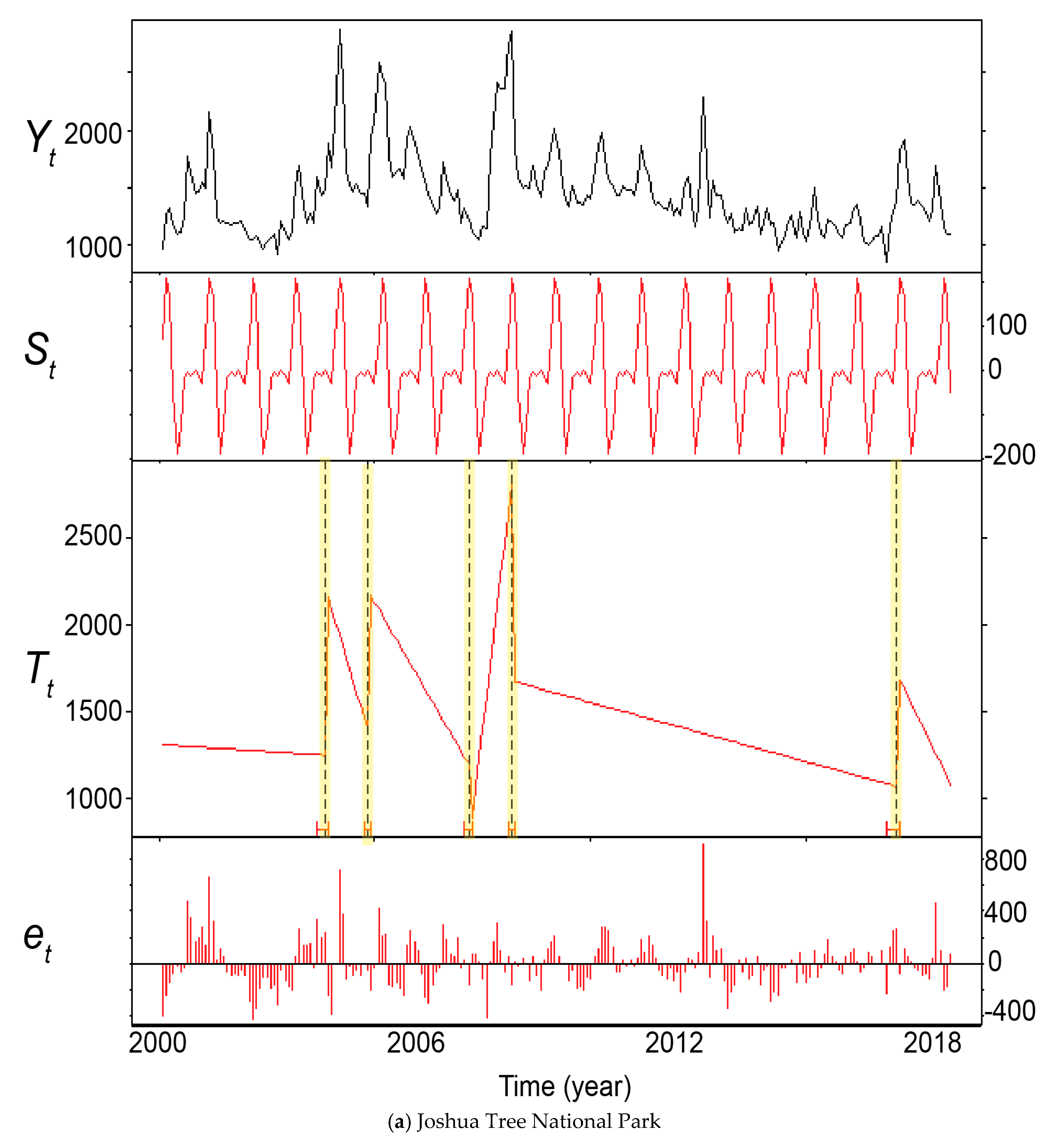
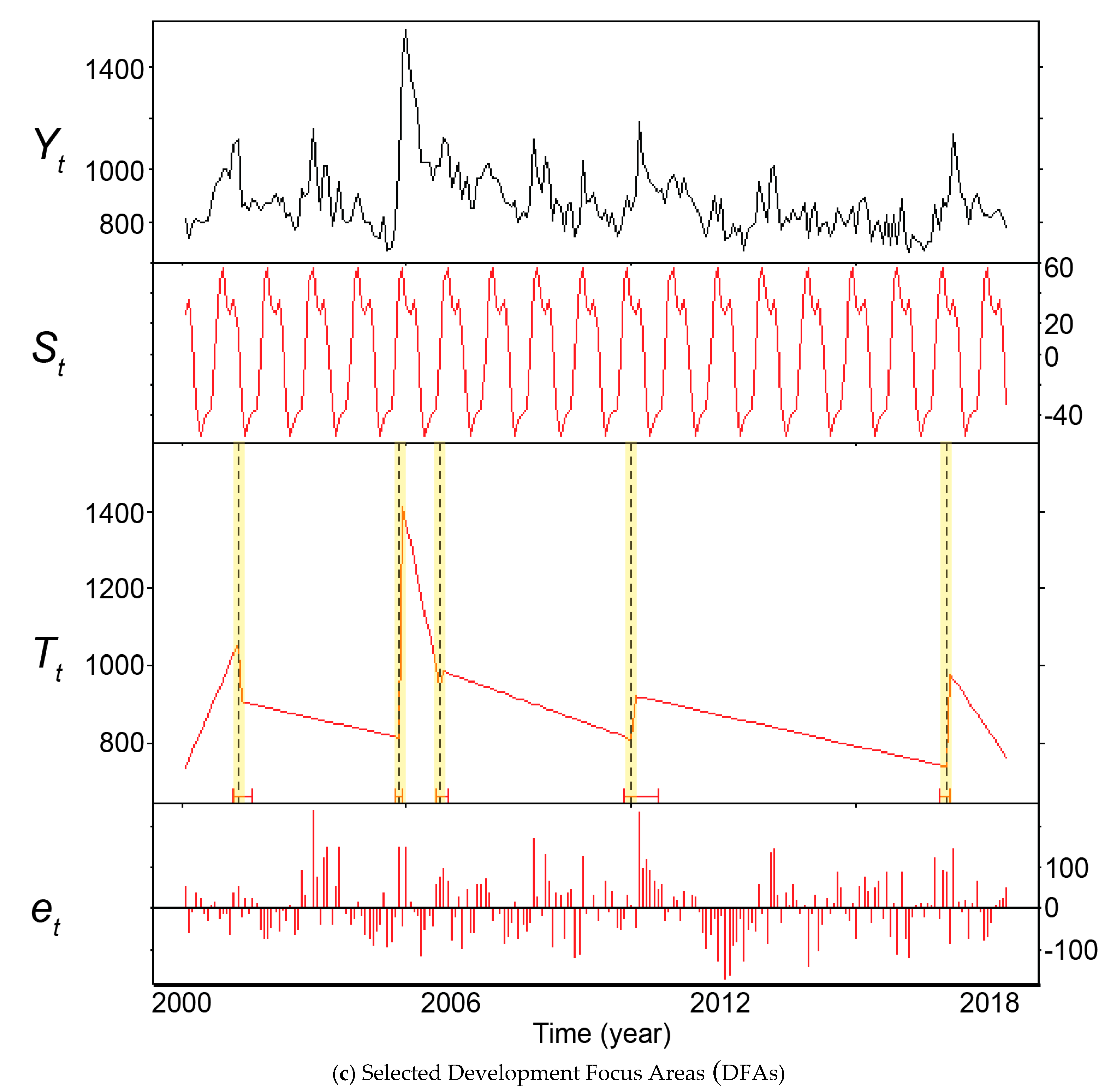
BFAST analysis was performed across the study regions using MODIS VI datasets for NDVI, EVI, and SAVI. Sample output results for JOTR, MOJA, and DFA sites illustrated the typical time series decomposition (
Figure 3). In general, the BFAST method tended to estimate five breakpoints, the maximum allowed, for each pixel in the study regions regardless of which VI was used. Specifically, the means of the total number of breakpoints for all study sites and all VIs were all larger than 4.5, with a maximum at the MOJA site of 4.96 breakpoints on average at a cell using the SAVI dataset.
The suitability of each VI for this study was assessed using sample cross-correlations with precipitation time series from nearby weather stations and comparisons against the timing of burns within fire boundaries. Precipitation should have a direct relationship with the VIs because greater rainfall tends to lead to more plant growth [
2]. Intense precipitation may waterlog plants and/or remove vegetation due to flood conditions, but these possible reductions in vegetation cover were considered as second-order impacts and thus not as influential. To compare the VI and precipitation time series by site, monthly precipitation time series were taken from three weather stations closest to each site (
Figure 1;
Table 2).
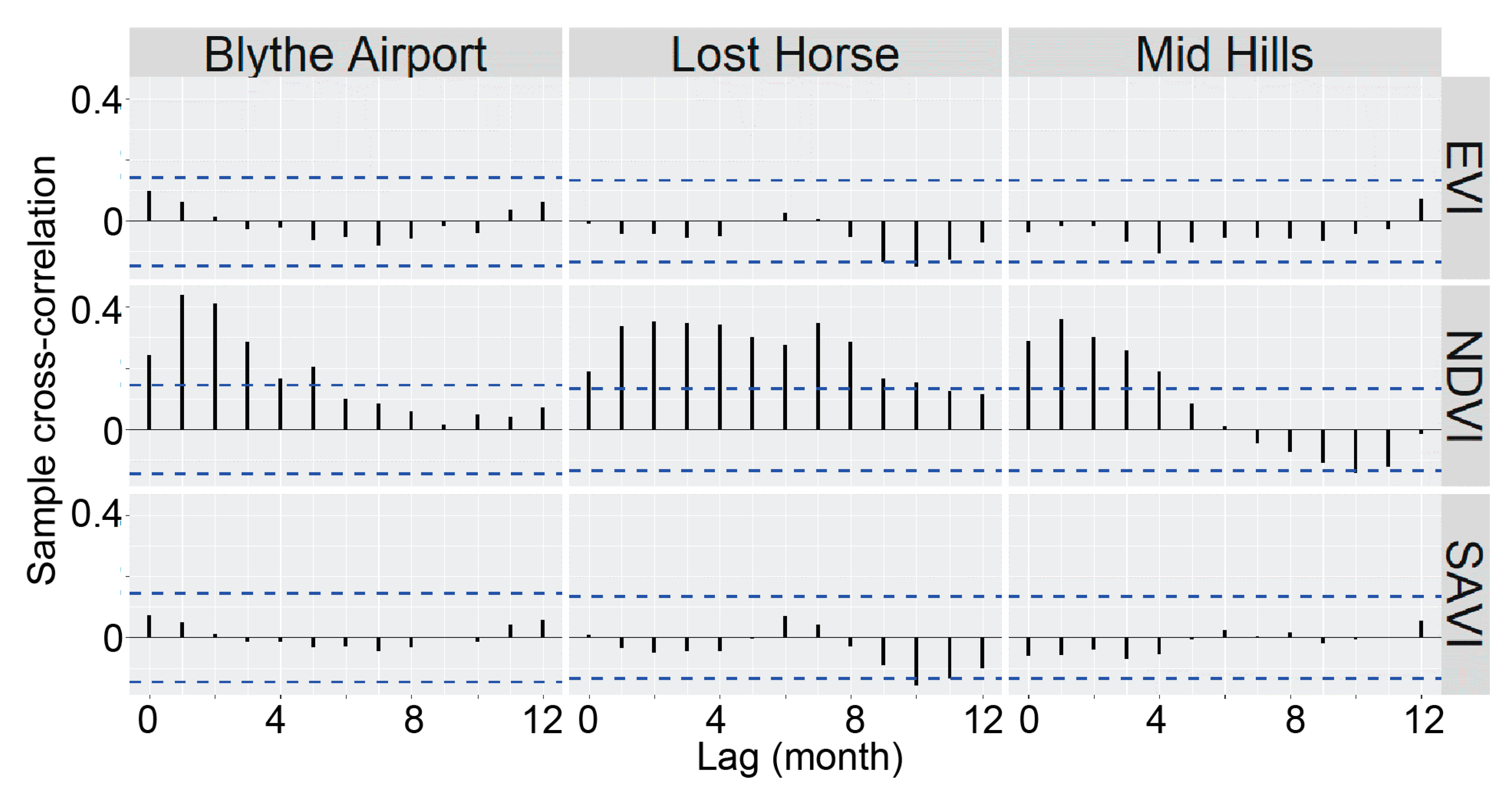
The sample cross-correlations between precipitation and the three separate VI time series showed that NDVI was best correlated with precipitation in terms of significant non-negative lags within one year (
Figure 4). The VI time series for comparison were aggregated as the mean of VI values in a 5 by 5 (1.25 km by 1.25 km) grid centered on the cell closest to the weather station. This spatial scale was selected to reduce any noise in the data while still remaining small enough remain within the same localized weather regime. Negative lags are not considered because, at a given time, precipitation should correlate with present or future responses in the VI. Lags were considered only if they were equal to or less than 12 months, as any lags afterwards would most likely not be related to precipitation response.
For all sites, sample cross-correlation between the NDVI and precipitation time series had significant positive correlation at non-negative lags (at the p < 0.05 level) within 0 and 4 months. On the other hand, EVI and SAVI time series did not have any significant positive correlation at non-negative lags. Even considering negative correlations, the EVI and SAVI time series had only one lag within a year (the 10-month lag) that had a significant negative correlation. The lack of significant negative correlations also supported the hypothesis that precipitation is more closely tied to vegetation greening rather than removal.
In addition, sample cross-correlations with breakpoint results were computed to directly compare change detection results for each VI with precipitation. For each VI, the breakpoint density time series was computed and the sample cross-correlation with precipitation was calculated. To gauge the impact of precipitation, which would tend to raise the VI value, only breakpoints that produced an increase in the VI were retained for this comparison. The sample cross-correlations between breakpoint density and precipitation indicated that the NDVI-derived time series had significant non-negative lags at all sites excepting the Mid Hills/Mojave site. The EVI-derived time series only had at least one significant non-negative lag within 12 months at the Mid Hills site, while the SAVI-derived time series had at least one lag fulfilling the criteria at the Blythe Airport/DFA site and Mid Hills/Mojave site.
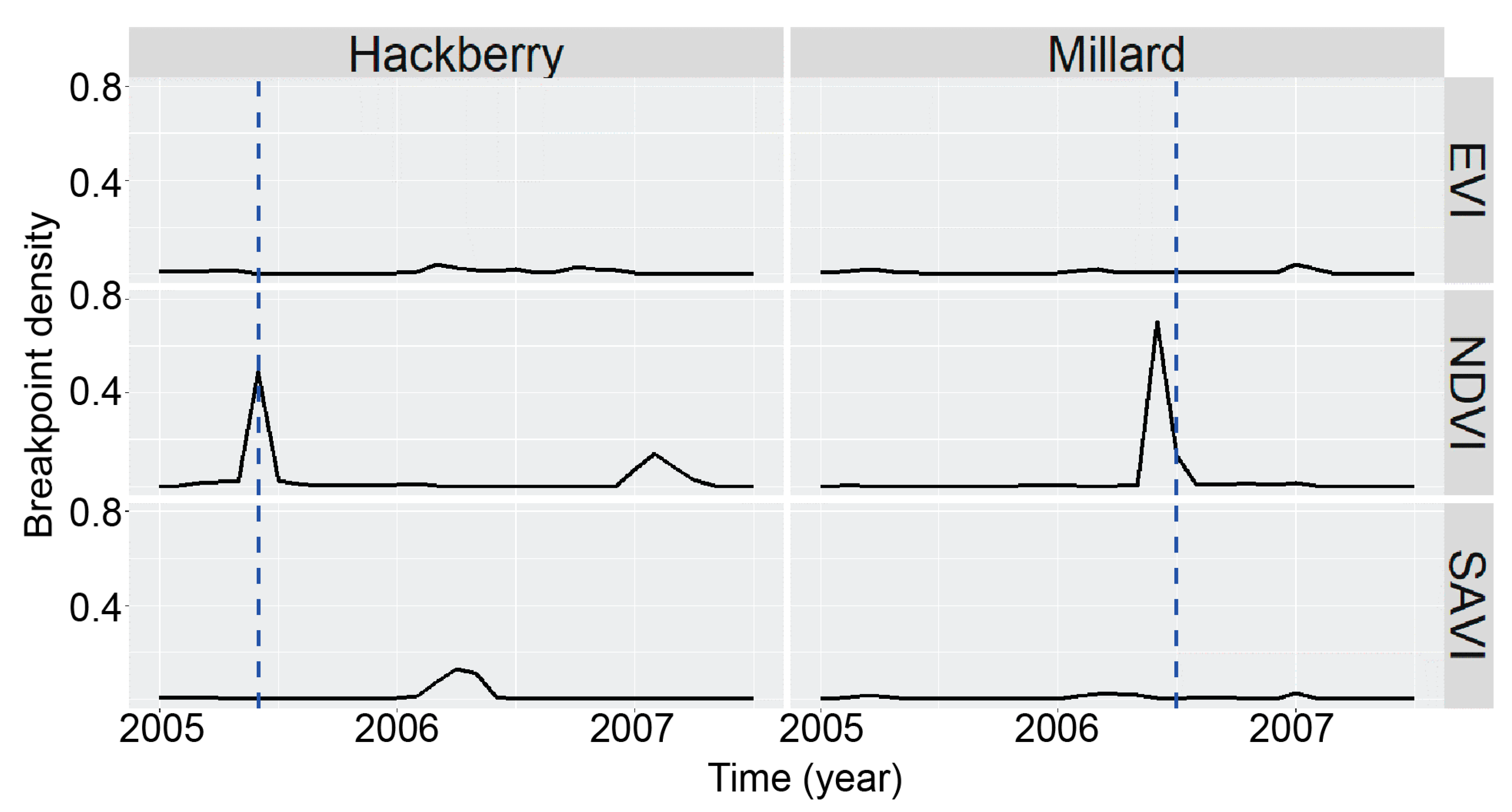
Comparisons between wildfire burns and VI time series were made at two burn sites, one near Joshua Tree National Park and the other in Mojave National Preserve (
Figure 1;
Table 3). The NDVI time series showed a peak of approximately 70% and 50% in negative breakpoint density around the corresponding month of burning for both the Millard and Hackberry fires, respectively (
Figure 5). In contrast, EVI and SAVI did not experience a peak at those times.
The combination of cross-correlation and wildfire results between the VIs supported the use of NDVI for further analysis because of their greater sensitivity in NDVI than EVI or SAVI to environmental perturbations. First, precipitation would tend to produce positive breakpoints at or after the corresponding time point in the positive breakpoint density. Consistent significant correlations at non-negative lags between positive breakpoint density from NDVI and precipitation supports application of NDVI. Although the NDVI breakpoint density time series was shown to be uncorrelated with precipitation at the Mid Hills MOJA site, the direct cross-correlation between NDVI and precipitation yielded the strongest relationship in terms of significant non-negative lags. The lack of a relationship between NDVI breakpoint density and precipitation at Mid Hills may arise from the assumption that precipitation will only produce positive breakpoints; any negative breakpoint response (e.g., flash flooding that uprooted vegetation) was not accounted for. Second, wildfires would tend to produce negative breakpoints. The fact that such major disturbances, at least in the two cases examined, registered in the NDVI (both in the VI itself and negative breakpoint density) but not EVI or SAVI additionally supported a focus on NDVI change for this study. All further analyses were performed using the MODIS NDVI dataset.
4.2. Change Detection at the Solar Energy Development Scale
Five solar energy sites (
Figure 1) were selected to examine results from BFAST change detection, each including a 2-km linear buffer from the visible perimeter of solar installations in which human disturbances related to solar energy development may operate as well. As a further note, the choice of such a “region of influence” was arbitrary so changing the scale of the analysis by varying the buffer distance may produce different conclusions as shown in the following results by examining sites with and without the buffer. Two additional sites from the JOTR and MOJA regions with similar area and low relief were included as controls. A hypothetical or “proxy” construction date was selected for the two control sites, as the date of the “start of construction” was assumed to be the construction date for the closest of the five solar energy sites. The selection of the control sites also assumed that the chosen area was similar in topography and land cover to those of the solar facilities. Therefore, the results on this subsection must be considered with these assumptions and limitations in mind.
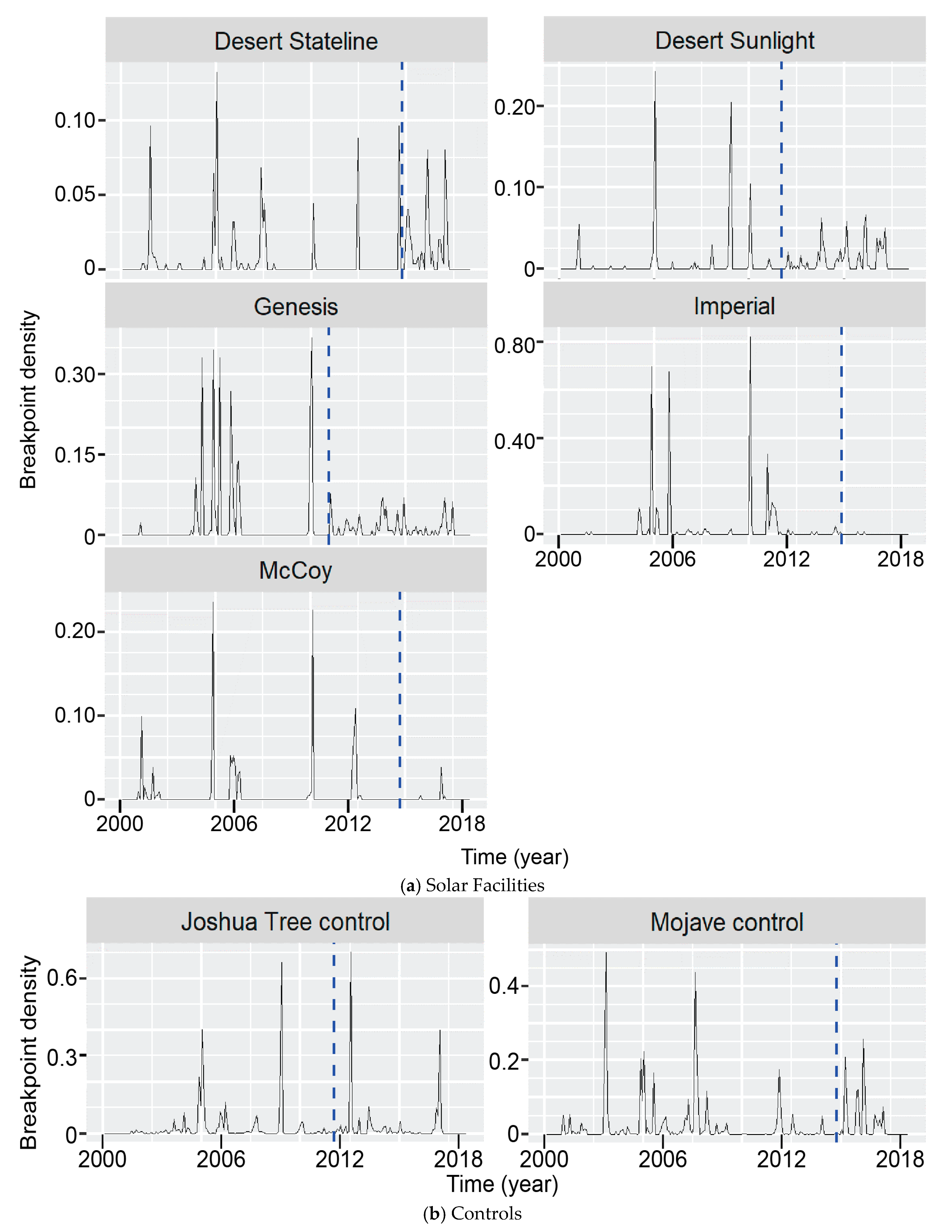
Time series of breakpoint density were plotted, and then segments of the time series were compared before and after the start of construction at each site (
Figure 6;
Table 4a).
The sign distribution of breakpoint shifts was not uniform across development sites (
Table 4b). The Desert Stateline and Desert Sunlight sites favored positive breakpoints (positive–negative ratio greater than 1) against negative breakpoints, but tended to favor negative breakpoints after construction of the solar facility. The Genesis site favored positive breakpoints before construction and continued to favor positive breakpoints afterwards. The results at the McCoy and Imperial sites could not be evaluated because of the sparsity of breakpoints after construction (10 and 2, respectively).
Variance in breakpoint density was computed for only the regions covered by solar installations for each site for the time series segment before the start of construction and after construction, and then evaluated for significance using a nonparametric bootstrap (
Table 4c). The time series of breakpoint density for each site was divided into a preconstruction and a postconstruction section, within which the variance was calculated. A bootstrap 95% confidence interval for the variance in the preconstruction segments was calculated and compared to the variance for the postconstruction segments. Inclusion of the 2-km buffer zone into the time series made the differences between pre- and postconstruction arbitrary and less clear.
For three out of the five solar energy sites, the postconstruction breakpoint density variance was significantly smaller than the preconstruction breakpoint density variance based on the 95% bootstrap confidence interval. In terms of vegetation cover, this result implies that, at these three sites, the variance has been significantly reduced due to a damping in the process tending to generate breakpoints. As this shift is aligned with the timing of the construction of solar energy sites, the result may relate construction to a reduction in breakpoint appearance. The Desert Sunlight and Desert Stateline sites did not reflect this pattern; their postconstruction breakpoint density variances were contained within the confidence interval. Likewise, the postconstruction breakpoint density variance was contained in the bootstrap confidence interval for both control sites.
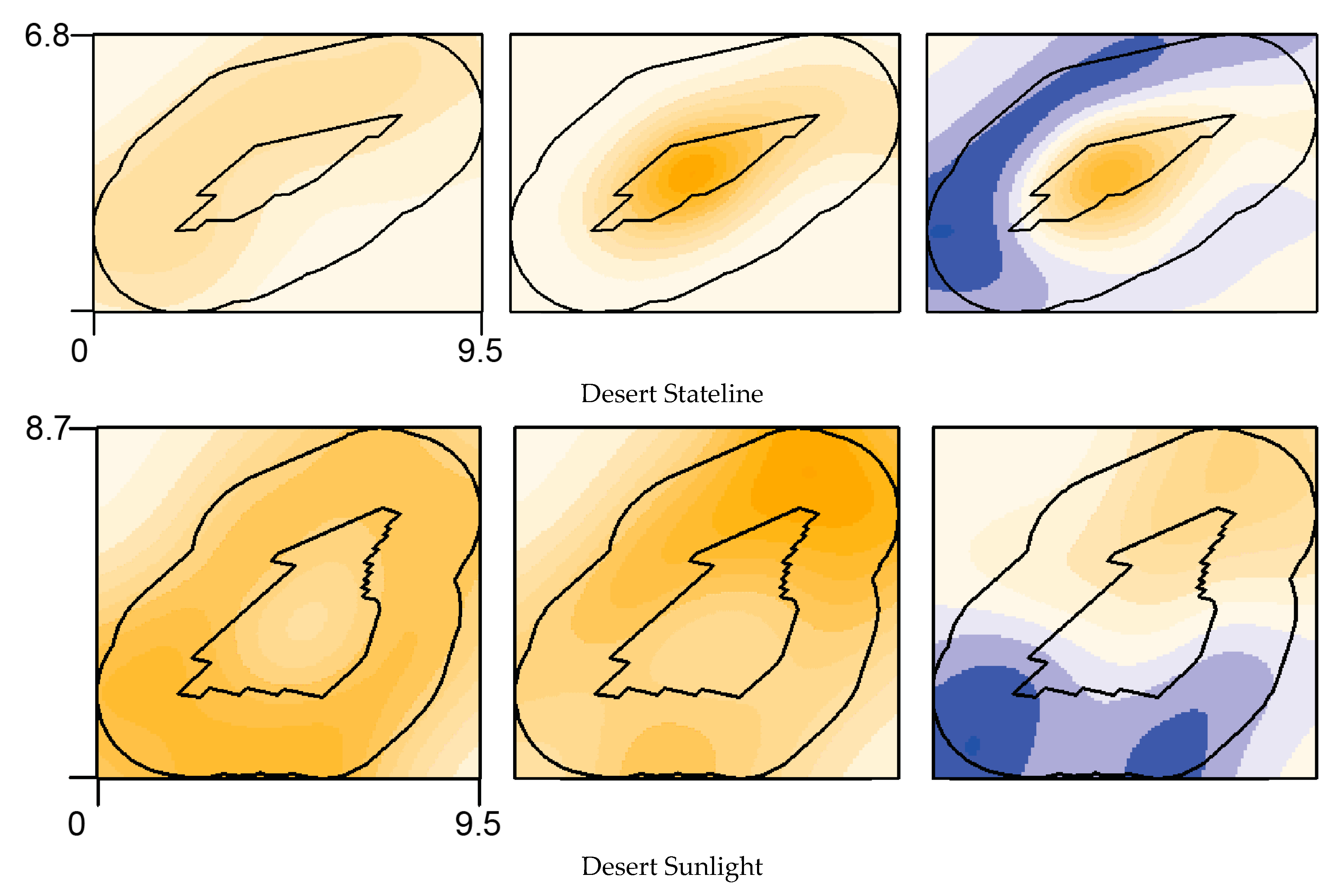
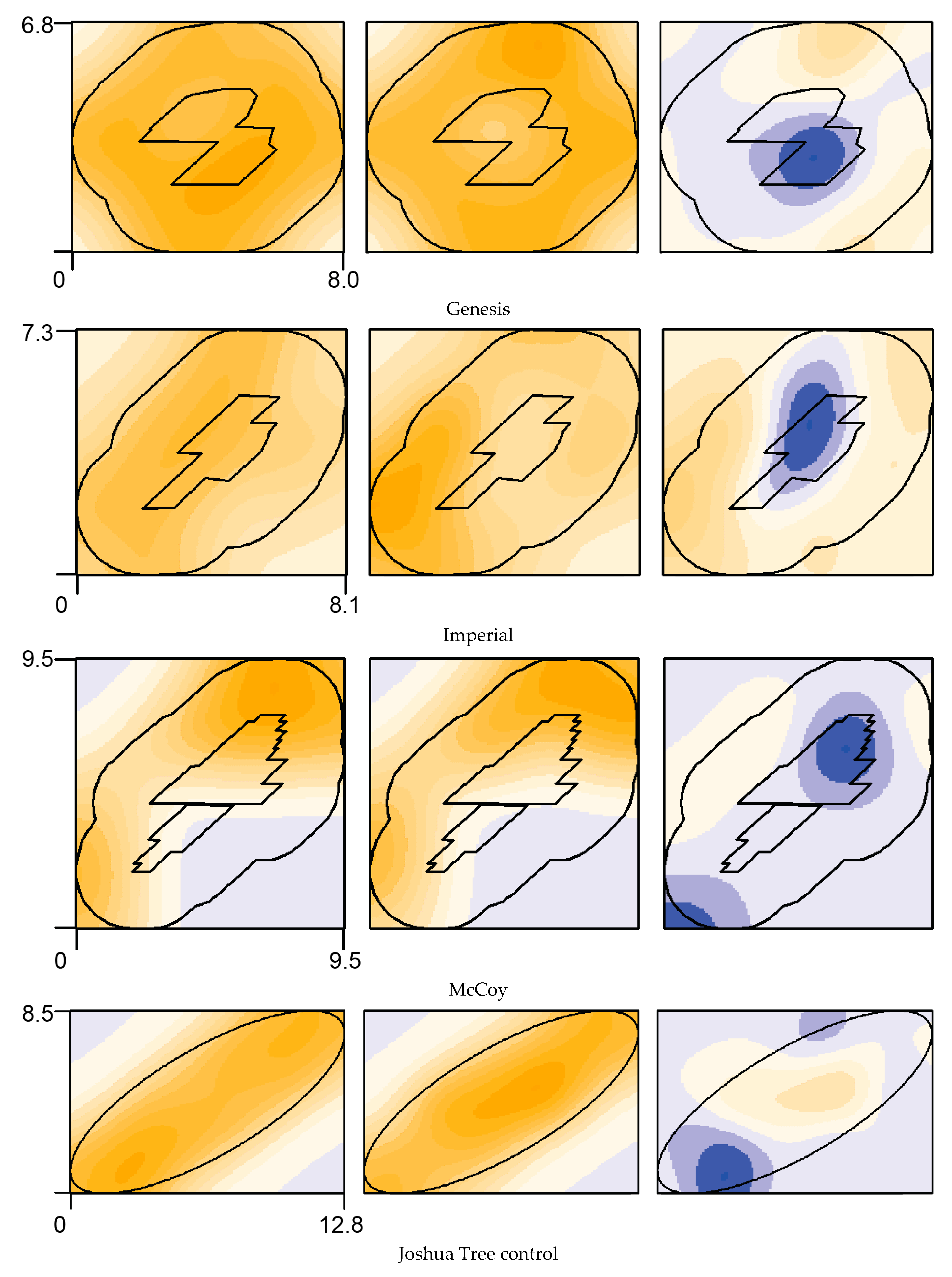
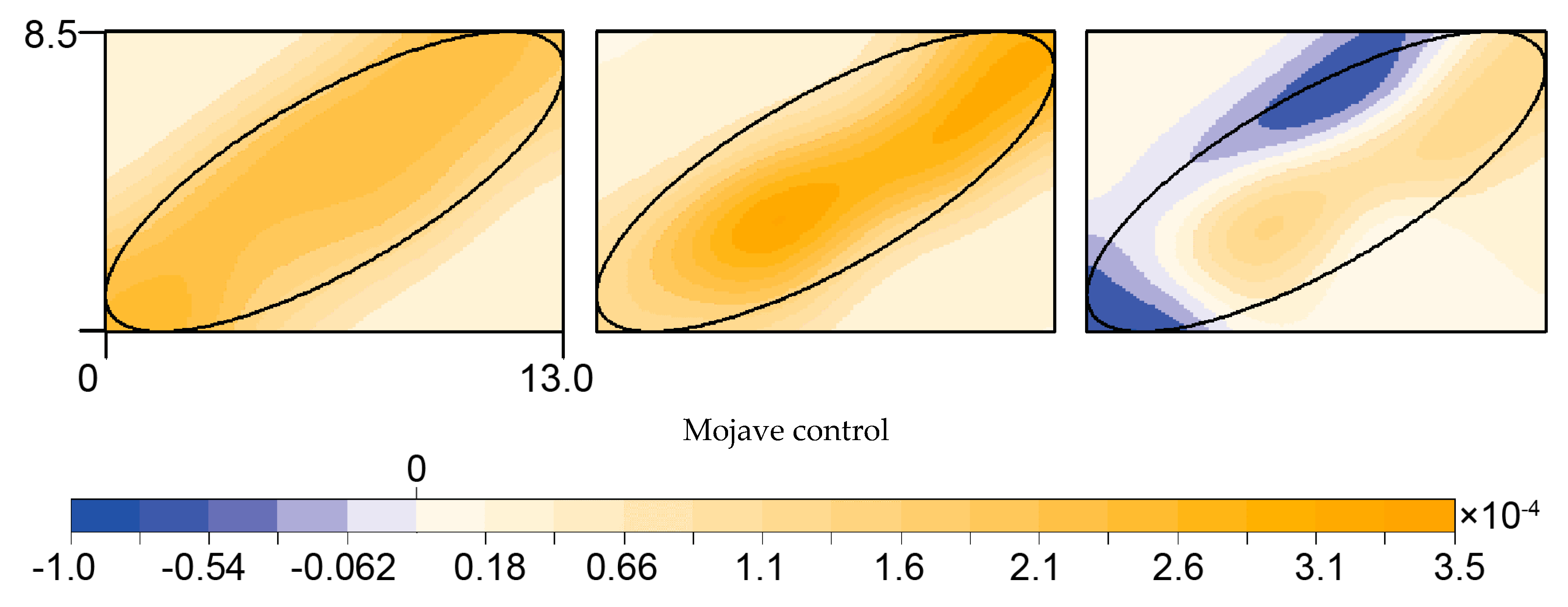
Kernel density estimation characterized the spatial distribution of breakpoints for all sites, but did not yield entirely consistent results (
Figure 7). The differenced breakpoint distributions directly on the solar installations at Genesis, McCoy, and Imperial Solar Energy Center West sites tended to concentrate negative values, indicating a reduction in breakpoint intensity over time. This pattern implies that the area of the solar installation footprints experienced a reduced intensity of breakpoints, thus less change in vegetation conditions, for those three sites. However, the Desert Sunlight and the Desert Stateline sites deviated from this general pattern. The kernel density estimates for Desert Stateline concentrated a greater mass of the distribution closer to the center of the solar installations after construction than before construction. The differenced distribution for the Desert Sunlight site indicated a shift in the distribution to the north.
The kernel density estimates for the control sites were also inconsistent. The Joshua Tree control site displayed a similar uniform breakpoint distribution before and after the proxy construction date. The density of the differenced surface indicated an approximately symmetric unimodal distribution centered at 0. The Mojave control site, before the proxy construction date, displayed a more uniform breakpoint distribution. However, the distribution was more concentrated away from the edges postconstruction. The density of the differenced surface indicated a less peaked distribution with greater spread across its range.
Despite the mixed results within each method, the McCoy, Genesis, and Imperial sites exhibited significant differences between pre- and postconstruction periods. This consistency implies that these sites experienced significant reductions of vegetation change in time and space at the solar installation footprints (referring to the two methods).
4.3. Change Detection at the Regional Scale
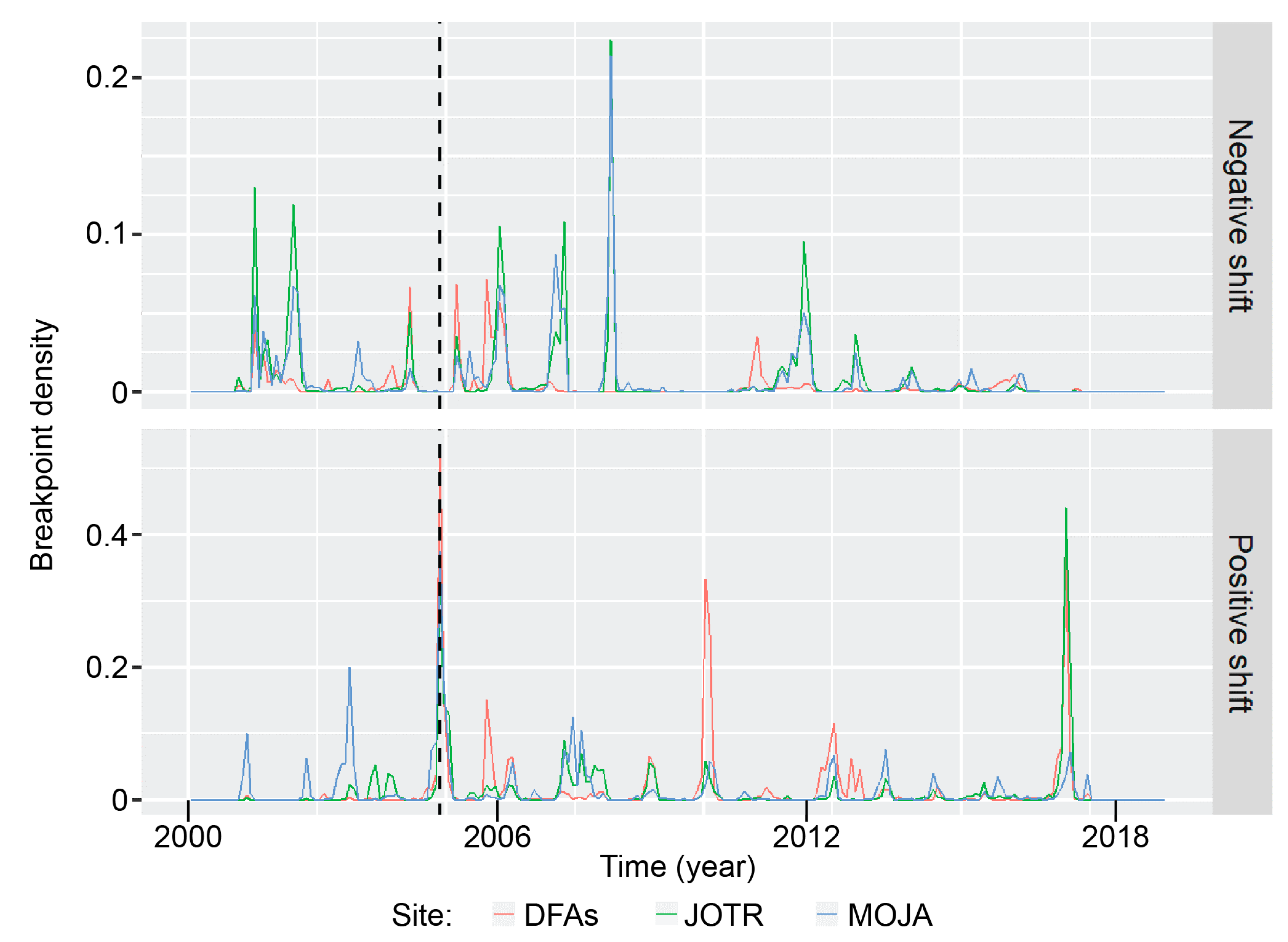
The BFAST method detected at least one breakpoint in 99% of the cells in the combined larger study areas (Joshua Tree National Park, Mojave National Preserve, and selected study DFAs). Time series of the breakpoint density for the study sites showed the presence of several large breakpoint events (
Figure 8). The positive breakpoint shifts were, in general, on a larger scale than the negative breakpoint shifts because their range extended up to about 50% coverage as opposed to only about 20% coverage for the negative shifts. The conspicuous peaks in the positive shifts were located approximately in late 2004 to early 2005, early 2010, and late 2016 to early 2017.
Distribution statistics for positive and negative change were computed and evaluated within the boundaries of the larger study sites to compare regional-level NDVI responses. For cells with multiple breakpoints, only the shift value with the maximum magnitude was retained to examine the most extreme breakpoint responses. Thus, the distributions were pooled over time to average out differential weather influences at finer temporal scales.
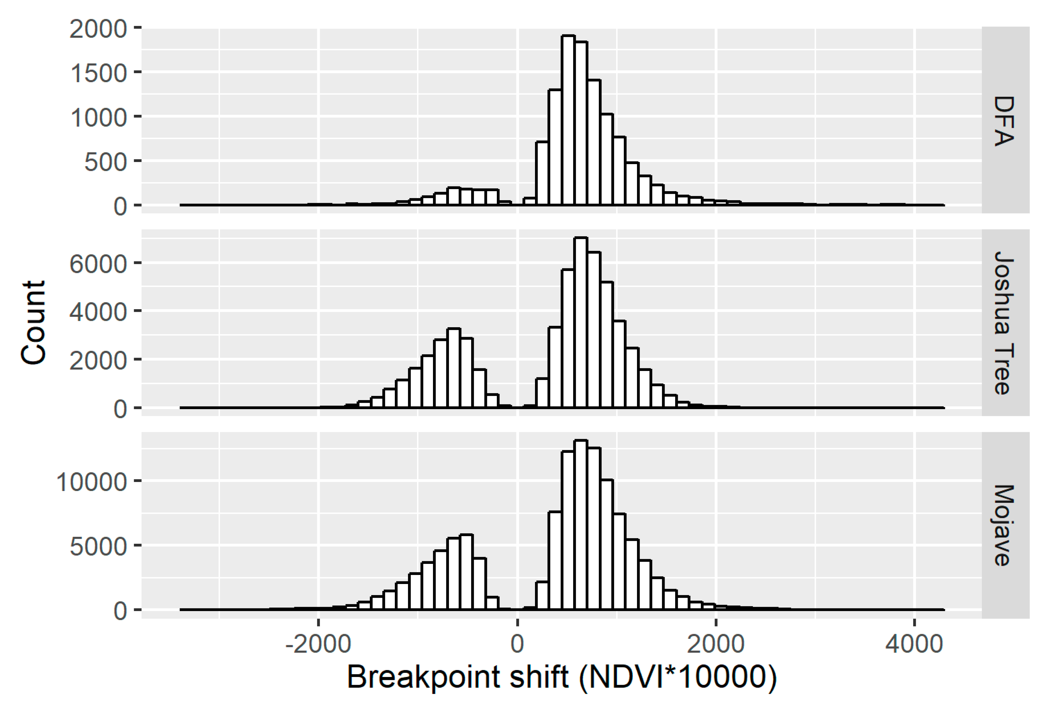
Histograms of breakpoint “shift” responses (change in a time series at a breakpoint) showed a bimodal distribution for all three sites (
Figure 9). However, the negative breakpoint shift response in the DFAs was less frequent than the positive shift responses. The distribution across the positive and negative breakpoint shift responses was more balanced in the case of JOTR and MOJA, but still favored positive shifts.
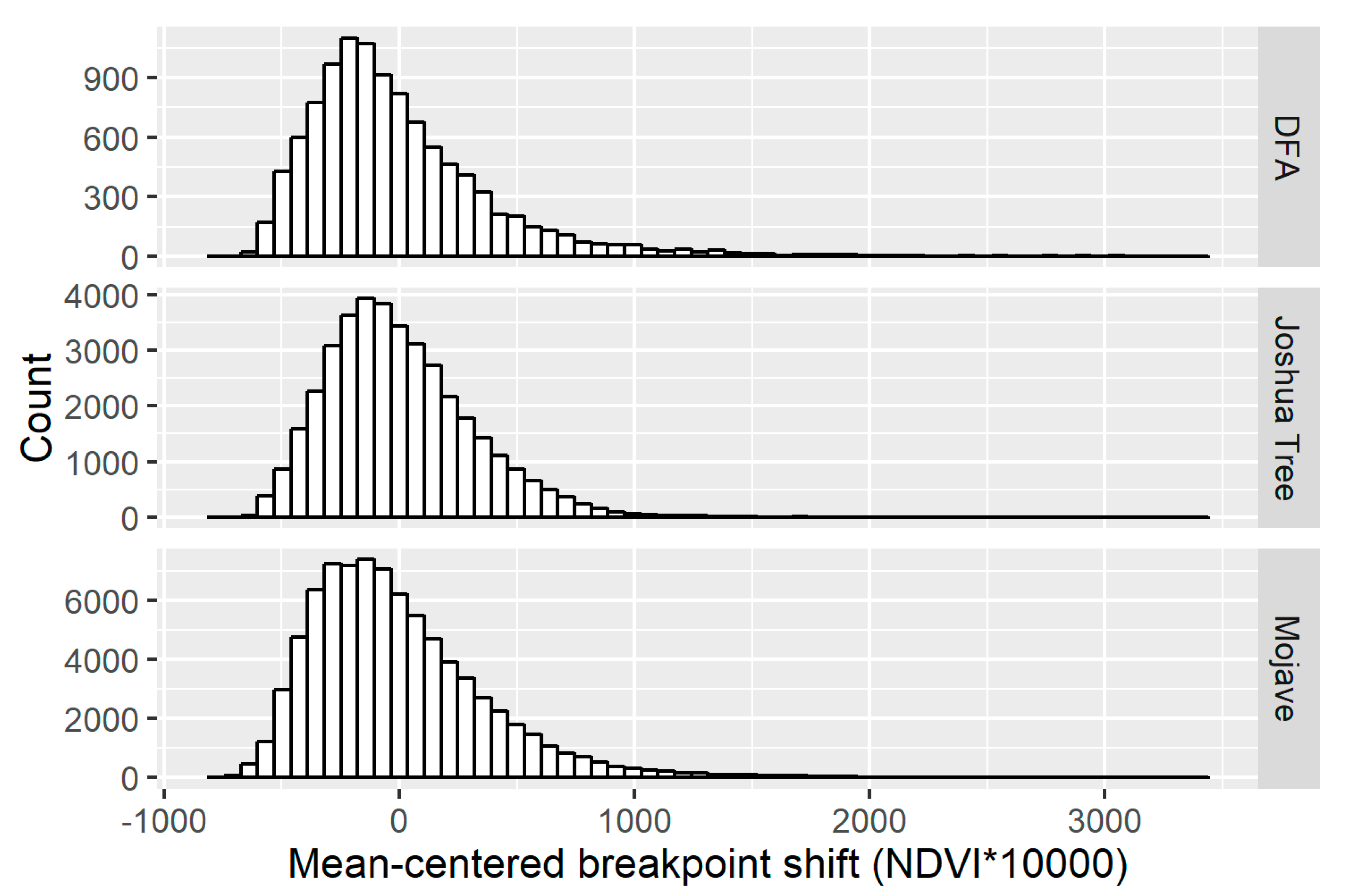
The overall breakpoint shift histogram was split into a positive and negative distribution and analyzed separately. The positive breakpoint distribution for all sites showed a right-skewed distribution (
Figure 10). The sample distribution statistics were also computed for a more precise distributional description (
Table 5a,b). The means between the three sample distributions are comparable, with a maximum range of 0.008 in NDVI (or 80 scaled NDVI units). However, the standard deviation, kurtosis, and skewness tend to set apart the sites more distinctly. The DFAs had the highest kurtosis, skewness, and standard deviation, followed by the MOJA and then JOTR. The skewness for all sites confirmed that the distribution in each site was right-skewed. All kurtosis values for distributions are leptokurtic, i.e., larger than 3, the kurtosis for a normal distribution.
A comparison of these summary statistics for the positive breakpoint shift distribution singled out the DFAs as having consistently greater “spread” statistics (standard deviation, skewness, and kurtosis) than the JOTR or MOJA sites. Bootstrap 95% confidence intervals for kurtosis and variance in the DFAs supported the fact that these statistics at the other sites were significantly smaller (
Table 5a). These numerical results imply that the DFAs, compared to the JOTR and MOJA regions, favored more extreme increases in NDVI and thus more intense greening episodes.
The same procedure performed on the positive breakpoint shift distribution was also applied to the negative breakpoint shift distribution (
Figure 11). The descriptive statistics for the distributions by site confirmed the visual observation that all three distributions are left-skewed (
Table 5b). The range in means was larger in the negative shift distributions than in the positive shift distributions (approximately 0.02 to 0.008 in NDVI), suggesting that negative responses were, on average, more variable between sites than positive responses. The kurtosis and magnitude of skewness were again largest for the DFAs, with JOTR showing the smallest values. The sample distributions were all leptokurtic, i.e., kurtosis values were all larger than 3. However, the MOJA site had the greatest variance, indicating that the negative shift distribution for this site had greater spread in values but thinner tails than that for the DFAs.
The nonparametric bootstrap did not significantly separate the sites in terms of kurtosis and standard deviation for the negative breakpoint shift distribution (
Table 5b). Although the DFA kurtosis was larger than that of the MOJA site and the DFA variance was smaller than that of MOJA, these differences were not significant according to 95% bootstrap confidence intervals. We did not find that, for the negative breakpoint distribution, the DFAs had significantly greater kurtosis and variance than both the MOJA and JOTR sites. These numerical results imply that, comparing both controls to the DFAs, declines in vegetation conditions operated on intensities that were indistinguishable from each other across sites.
5. Discussion
5.1. Vegetation Index Suitability
Correlations with precipitation and wildfires support the use of NDVI instead of EVI or SAVI within the study region, a finding that may be attributable to its dynamic VI range. Huete et al. [
12] found that the NDVI product from the Terra MODIS sensor tends to have a greater range in values in their semiarid study sites than did EVI. Thus, the higher sensitivity of NDVI to these events may stem from its stronger signal in the presence of sparser vegetation cover typical of desert ecosystems. Another contributing factor may be the more uniform structure of vegetation in the study area. In practice, EVI and SAVI are more sensitive to differences in vegetation structure, such as canopy architecture [
12,
13]. In contrast, NDVI relies more on variations in chlorophyll to distinguish values. Since a substantial portion of the study area is dominated by low, sparse vegetation like creosote bush and white bursage, structural variations are more uniform than are variations in chlorophyll. Then, EVI and SAVI may appear less sensitive because vegetation structure is less variable than chlorophyll content. This reasoning would explain the insensitivity of EVI and SAVI to the examined wildfires (
Figure 5).
The tendency of SAVI to yield similar breakpoint results to EVI may be due to the common feature of SAVI and EVI for decoupling the vegetation signal from the background canopy [
13]. EVI and SAVI may be more suited for detecting different types of vegetation change and warrant evaluation in this regard. One well-documented guideline is that EVI would be more appropriate for regions where vegetation is denser and greener because NDVI tends to saturate whereas EVI remains responsive in those conditions [
12]. Nonetheless, suitability assessments for other VIs must be completed to optimize the correlation between a VI and vegetation characteristics (e.g., density, diversity, height) that may be influential for ecosystem functioning.
5.2. Meteorological Controls on Breakpoints
The regional-scale analysis of Joshua Tree National Park, Mojave National Preserve, and the selected DFAs supports the idea that anomalously large precipitation events tend to dictate the appearance of (positive) breakpoints. The positive peaks in the breakpoint density for these sites were located in three time periods associated with generally higher than average rainfall totals, namely the 2005, 2010, and 2017 water years. Thus, these major peaks are correlated with higher than average rainfall seasons.
In addition, the ubiquity of cells with at least one breakpoint (99% for these study regions) implies a phenomenon, like precipitation, operating on the scale of hundreds of thousands of square kilometers. Although the BFAST method incorporates seasonality in estimating breakpoints, these elevated precipitation intensity events are not captured in the seasonal model because of their lower frequency. This outcome may be a feature, if one wishes to track deviations from the usual yearly cycle, or a drawback, if one wishes to completely decouple the vegetation signal from the precipitation cycle. A more detailed harmonic model fit that includes more frequencies may be necessary for the latter case.
The causes of negative VI breakpoints in our study region are less clear because of the lack of any single particular phenomenon that reduces NDVI at the regional-scale. Two plausible mechanisms for negative breakpoints are drought and wildfires. Wildfires, although they do influence a landscape at the scale of analysis addressed by MODIS, do not occur as often in a daily, widespread fashion as does a heavy rain event, thus making fire impacts more difficult to pinpoint in the time series. NDVI reduction due to drought is also difficult to attribute in the time series because the browning is gradual, making the expression in breakpoints less clear. A combination of drought and wildfire may have a unique signature as well in the time series, but is not readily identifiable from the data.
5.3. Surface Homogeneity at the Scale of Solar Energy Development Sites
The BFAST variance results showed that the postconstruction variances in breakpoint density were significantly smaller than the preconstruction variances for the solar installations at all sites except Desert Sunlight. For the facilities at which this pattern did hold, the reduction in breakpoint density variance may be attributable to an effective “homogenization” of the desert surface. The introduction of an expanse of solar installations, whether concentrated or photovoltaic, would smooth out the differences in the natural desert landscape by masking any underlying vegetation signal and reduce surface variability overall simply by virtue of their identical construction. The notion that construction of new road surfaces is not a major factor in NDVI change is supported by the lack of a coherent difference between pre- and postconstruction breakpoint density time series because the buffer areas immediately surrounding the solar installations, but not covered by them, would not have been transformed into such a uniform surface by road traffic and land clearing for equipment usage.
This causal effect of a homogenized surface was supported by the kernel density estimates. The variance results reveal that breakpoint events produce far fewer breakpoints in a given area after the construction of solar installations. The spatial kernel density estimates answer where the breakpoint distribution changes. The differenced probability surfaces for Genesis, McCoy, and Imperial sites showed that breakpoints, when they did occur after construction, tended to occur away from the solar installations themselves compared to the distribution before construction. This finding was consistent with the apparent decrease in breakpoint density variability after the start of construction.
The above findings do not apply to the Desert Sunlight and Desert Stateline sites because they do not follow the observed pattern of reducing breakpoint influence at the solar installations. The Desert Sunlight site did not have a significantly smaller postconstruction breakpoint density variance and did not show a clear reduction in breakpoint probability density over solar installations from before and after construction. We expect that this discrepancy stems from the specific construction process of the site. Desert Sunlight had a nominal construction start date of September 2011. However, Landsat imagery taken in May 2012 shows that a vast majority of the solar installations had not yet been installed but were beginning to be placed onsite from the southern margin. This fact may account for the differential north-south gradient in the differenced density surface for Desert Sunlight. Since the southern half of the site had been developed and impacted first, it exhibited a stronger reduction in breakpoint occurrence than the northern section.
The Desert Stateline site seemed to concentrate breakpoints where solar installations were located rather than disperse them according to the differenced density surface. One possible reason for this apparent discrepancy is the presence of a medium-sized road running north–south through the center of the facility (diagonal from southwest to northeast in the plots due to the MODIS spatial projection), with an appreciable margin of unpaved desert surface to the sides. Thus, any vegetation signal at the site would be expressed through this section of exposed ground, potentially accounting for the concentration of breakpoints toward the center.
Overall, the change detection results at Desert Stateline and Desert Sunlight tended to be different from those at the other solar sites, not simply in regard to density estimation. The ratio of positive to negative breakpoints at these two sites changed dramatically from being much larger than 1 (about 3 and 9) prior to construction to being less than 1 after construction. Furthermore, these two sites were the only solar energy facilities in the study whose postconstruction breakpoint density variances were comparable to their preconstruction breakpoint density variances. These findings imply that Desert Stateline and Desert Sunlight tended to maintain similar breakpoint variability with time, but the mechanism behind the breakpoints tended to reduce NDVI instead of increasing it. This shift could signal a change in the “breakpoint generation process” from precipitation-dominated (positive breakpoints) to human-dominated (negative breakpoints).
5.4. Positive Breakpoint Distribution
The significantly larger kurtosis and variance in the DFAs for the positive shift distribution suggest that the DFAs have had a more extreme positive NDVI response to the positive shift events (precipitation, in most cases) than the MOJA and JOTR sites. The similar means across sites imply that, on average, the positive NDVI shifts are similar in all sites but the tendency for greater variance and kurtosis in the DFAs, combined with high skewness, implies that shifts greater than the mean were more common in the DFAs. This conclusion is supported by the bootstrap distributions for the variance and kurtosis in the DFAs, strongly suggesting that the variance and kurtosis in the DFAs are significantly greater than those of the MOJA and JOTR sites.
One potential explanation is that vegetation health and density in the DFAs are, in general, lower than those in protected regions, a claim that is supported by NDVI observations and the legacy of human activity. The mean MODIS NDVI, after spatial and temporal averaging, was lowest for the DFAs, with the MOJA site having the largest value (
Table 6). Moreover, portions of the DFAs have been subject to extreme human disturbances dating back to World War II, when the region was utilized as a military training ground and experienced heavy vehicle use and explosive bombardments [
26]. The positive shifts in the DFAs could tend to larger values because any particular amount of rainfall would produce a stronger response in the more damaged vegetation conditions. For example, a similar precipitation event would produce a much lesser NDVI response in healthy vegetation than in browning vegetation, in which an input of the same amount of water would allow it “green up” and begin to recover. JOTR protects stands of denser woodlands than are seen in the DFAs. The explanation above would also align with the fact that JOTR has the lowest kurtosis and variance in positive shift distribution out of the three sites (JOTR, MOJA, and DFAs).
The MOJA site was shown to have the highest mean NDVI among the study sites, but did not have the smallest sample kurtosis and variance. Slightly cooler summer temperatures and higher average annual rainfall in the eastern Mojave may account for this paradox. Higher elevations and cooler temperatures at MOJA could reduce the rate at which the soil dries out following precipitation, making more water available to plants over a longer period of time. Furthermore, extreme NDVI shift values were relatively rare as a result, because soil water is available for longer, reducing the burden for the plant to uptake the water quickly. This more dispersed greening from the feedback between water availability and temperature explains the apparent discrepancy between the NDVI and distributional statistics across sites.
5.5. Negative Breakpoint Distribution
Negative shift responses seem to be less favored overall in the DFAs compared to the protected sites, but the level of response seems to be comparable to the MOJA site when negative shifts do occur. As seen in the overall histogram of shifts by site, the ratio of negative to positive shifts is smaller in the DFAs than in other sites, where the ratio tends to be closer to 1. Negative shift responses could be less dominant in the DFAs because of the presence of developed areas. Events that could lead to a sharp decline in vegetation conditions would be more controlled and mitigated for by humans. Decreases in vegetation density and health during drought could be more muted because of poorer initial vegetation conditions in the DFAs, so there is less potential for a major drop in NDVI.
5.6. Limitations and Future Work
Field studies of the specific areas of interest were outside the scope of this study. Future work should elucidate the connection between the purely statistical concept of a breakpoint with the possible suite of physical phenomena it may represent. As a result, the conclusions drawn here, although plausible, remain tentative until detailed fieldwork is performed for validation. Once the bridge between the statistical and physical meanings is clarified, the methods presented here will be valuable and practical tools to monitor sustainable development.
While a remote sensing framework using vegetation index datasets has been presented here, the analysis relies on the suitability of vegetation indices as a proxy for vegetation conditions. More lines of inquiry, for example, data on soil moisture and surface temperature, are required for a comprehensive evaluation that vegetation indices alone cannot give. As BFAST only supports univariate time series, further work should develop multivariate time series approaches to incorporate relevant data to capture the wider collection of possibly influential processes.
6. Conclusions
A remote sensing change detection framework based on the BFAST time series analysis method was developed and applied to identify the ecosystem impacts of solar energy sites in southern California deserts. Three VIs (NDVI, EVI, and SAVI) were tested for their sensitivity to precipitation and wildfire perturbations. NDVI was shown to have the strongest response, and thus adopted for the subsequent analysis. The Terra MODIS NDVI dataset, starting from 2000, was used in the BFAST change detection approach, which estimated breakpoints independent of seasonality. The BFAST change detection analysis showed that positive breakpoints in NDVI are correlated with larger than average rainfall events regardless of protection status, but negative breakpoints tended to have more clearly different responses in JOTR, MOJA, and the selected study DFAs. The positive breakpoint shift distribution for the DFAs indicated significantly larger variance and kurtosis. On the other hand, the statistics for the negative breakpoint shift distribution for the DFAs could not be significantly differentiated from the protected lands apart from the fact that negative breakpoints were less frequent compared to positive breakpoints. These results may stem from differences in baseline vegetation conditions and prior degradation. At the scale of individual solar energy sites, breakpoint patterns were less consistent. Three out of the five solar energy facilities examined indicated that the distribution of breakpoints after construction, when breakpoints did occur, were focused away from the immediate location of solar installations. This phenomenon may be linked to a “homogenization” of the desert surface, a transformation that would inhibit the appearance of breakpoints. However, the presence of sites that do not match this pattern points to the significance of site-specific factors in determining the response to construction. Finally, fieldwork is a key next step to connecting the largely statistical analysis of this study with the physical significance to the desert ecosystem at the ground level.


