
Leaf Wetness Evaluation Using Artificial Neural Network for Improving Apple Scab Fight
by
 ,
,
Alessandro Stella
1, 
Gennaro Caliendo
1,
Farid Melgani
2,*,
Rino Goller
1,
Maurizio Barazzuol
1 and
Nicola La Porta
3,4
1
Metacortex S.r.l., Via dei Campi 27, Torcegno 38050, Italy;
2
Department of Information Engineering and Computer Science, University of Trento, Via Sommarive, 9,Trento 38123, Italy
3
Iasma Research and Innovation Centre, Fondazione Edmund Mach, Via E. Mach 1, San Michele all’Adige 38010, Italy
4
Mountfor Project Centre, European Forest Institute, Via E. Mach 1, San Michele all’Adige 38010, Italy
*
Author to whom correspondence should be addressed.
Environments 2017, 4(2), 42; https://doi.org/10.3390/environments4020042
Submission received: 29 April 2017
/
Revised: 8 June 2017
/
Accepted: 10 June 2017
/
Published: 13 June 2017
(This article belongs to the Special Issue Information and Communication Technologies for Improving Monitoring and Management Schemes in Agricultural Environments)
Abstract
:Precision agriculture represents a promising technological trend in which governments and local authorities are increasingly investing. In particular, optimising the use of pesticides and having localised models of plant disease are the most important goals for the farmers of the future. The Trentino province in Italy is known as a strong national producer of apples. Apple production has to face many issues, however, among which is apple scab. This disease depends mainly on leaf wetness data typically acquired by fixed sensors. Based on the exploitation of artificial neural networks, this work aims to spatially extend the measurements of such sensors across uncovered areas (areas deprived of sensors). Achieved results have been validated comparing the apple scab risk of the same zone using either real leaf wetness data and estimated data. Thanks to the proposed method, it is possible to get the most relevant parameter of apple scab risk in places where no leaf wetness sensor is available. Moreover, our method permits having a specific risk evaluation of apple scab infection for each orchard, leading to an optimization of the use of chemical pesticides.
1. Introduction
Apple scab is one of the worst issues that can occur in apple orchards and also during postharvest. Such kinds of diseases can give rise to black or grey fungal lesions on leaves and fruits, thereby diminishing significantly fruit yields and quality therein. In some cases, it can even lead to a complete defoliation of apple trees. Apple Scab is caused by the Ascomycete fungus Venturia Inaequalis that appears in springtime under suitable temperature and moisture, resulting in Ascospores conditions [1]. Ascospores attack tree tissues, and if the plant is wet, infection takes place [2]. Unfortunately, curative treatments are not really effective. Moreover, they can be applied only a few times in a season [3]. Consequently, the only type of treatment that can help tackling such an issue, especially at the early stages, is preventive treatment. However, spray timing has to be calculated accurately so that it would be performed within 90 h. Having a correct way to evaluate infection risk is therefore important to promptly prevent apple scab effect and also to reduce the amount of used pesticides [4,5].
On the other hand, scab disease is mainly affected by leaf wetness data that measures the wet period duration (in minutes) of the leaf surface. Nonetheless, the main problem with this kind of data is that it strongly depends on the position of the weather station where leaf wetness sensor is placed. In particular, as a matter of fact, leaf wetness measurement is extended to kilometers from one station to another. In a region like Trentino, where weather is strongly heterogeneous, inducing numerous micro-climates, this kind of approach leads to a wrong evaluation regarding the risk of infection. In this paper, the aim is to use advanced technologies to improve pre-existent risk evaluation models. Particularly, using the A-Scab model [6] as a starting point, we develop a way to extract local data from UAV (Unmanned Aerial Vehicle) imagery survey (produced according to ENAC (Italian Civil Aviation Authority) restrictions for non-critical environments) [7]. Furthermore, we develop a method to extend weather station data to places that lack it. The parameter that plays a fundamental role in scab risk evaluation is leaf wetness duration, which, as mentioned earlier, is the main condition behind an infection case. Our method consists of training an artificial neural network (ANN) so that it will take hourly weather data from the neighbouring weather station and the geographical position of the orchard of interest as input, and returns the hourly estimated leaf wetness as output. Thus, it is possible to geographically extend and generalise the apple scab risk infection model, while also obtaining leaf wetness forecast data.
2. Materials and Methods
2.1. Risk Evaluation Model
To better understand how the evaluation of risk infection works and how leaf wetness values influence its computation, it is important to introduce the A-Scab model [6]. Such a model has been developed by the University of Piacenza (Italy) and is aimed at evaluating the apple scab infection risk. The innovation behind such a technique is that it depends only on the weather data and no tuning or calibration is necessary. Moreover, it is the only prevision model that is supported by scientific publications. The pipeline of A-Scab is illustrated in Figure 1:
First, weather data are hourly acquired from weather stations, and the beginning of infection is simultaneously determined, using the equations reported in [8]. After this procedure, the model waits for an infection event to occur. When this happens, using indices like PAT (Proportion of Ascospores that has been Trapped) and LAI (Leaf Area Index), risk infection severity and symptom appearance dates are computed.
Leaf wetness (min) plays a fundamental role in the apple scab risk evaluation model. This kind of data is typically acquired with a special sensor that emulates the overall radiation balance of a healthy leaf, so moisture will condense and evaporate from the sensor at the same rate as it would on a normal leaf.
Principally, there are two main problems regarding such sensors:
- They need specific and periodic maintenance (i.e., dirty or improperly installed sensors lead to incorrect values).
- In a territory like Trentino, which has many micro-climates, the leaf weather data is highly variable and can not be easily extended to zones where no sensor is available.
The first problem strongly depends on the single weather station owner and it could be resolved by carrying out a proper sensor maintenance. Thus, assuming that leaf wetness data acquired by a sensor placed in a specific location is reliable, the solution to the second problem is the subject matter of this work.
Prior to discussing the adopted strategy, it is important to understand how leaf wetness is used in the A-Scab model to evaluate the infection risk. First of all, leaf wetness is used to compute the proportion of Ascospores that can potentially become airborne (PAT = Proportion of Ascospores that has been Trapped) [3,9]. PAT index represents indirectly the dynamic of Ascospores maturation and their risk potentiality. This index is computed as follows:
where is temperature at each hour (h) of the day with inferior limits 0, and is a binary index equal to 1 if, at hour h, there is wetness on leaf surface; otherwise, it is equal to 0. As it is, it could be noticed that an incorrect value of leaf wetness leads to a wrong estimation of the dynamic of Ascospores maturation. PAT value is also used to directly evaluate the Ascospore dose ejected during a discharge event (). Another infection risk evaluation parameter where leaf wetness plays a fundamental role is the infection efficiency of Ascospores deposited on apple leaves. In fact, in order to verify the possibility for Ascospores to cause infection, it is necessary that, during a discharge event (period with lasting one to several hours, interrupted by a maximum of two hours), there has to be two wet periods interrupted by a dry period of at least four hours; shorter interruptions of wet periods are not considered as interruptions. The total amount of leaf wetness hour during an infection period () defines minimum conditions for infection of apple leaves by Ascospores to occur according to the Stensvand Table [10]. This data is also used to directly compute the hourly amount of germinated Ascospores () and the amount Ascospores with Apressorium (). Moreover, is used to compute indirectly the mortality rate of Ascospores at stage (non germinated Ascospores), , [11]. As shown above, the leaf wetness is part of many parameters used in the risk infection evaluation model that computes the severity of possible risks as follows:
where is the value of at the end of infection period, is the host susceptibility computed using LAI (Leaf Area Index) and n is the number of days including the infection period.
2.2. Artificial Neural Network for Leaf Wetness Estimation
Due to its relevance and to its variability in regions like Trentino, it is important to design a model that can extend leaf wetness value to lacking zones. To this end, we opt for an artificial neural network approach, and, more particularly, the Multi-Layer Perceptron Network (MLP) [12].
Such kind of network has been favoured over other networks (e.g., radial basis function neural network, general regression) due to its excellent capability of modelling any kind of function at any complexity level as long as the training set is of the proper dimension (as in our case) [13,14].
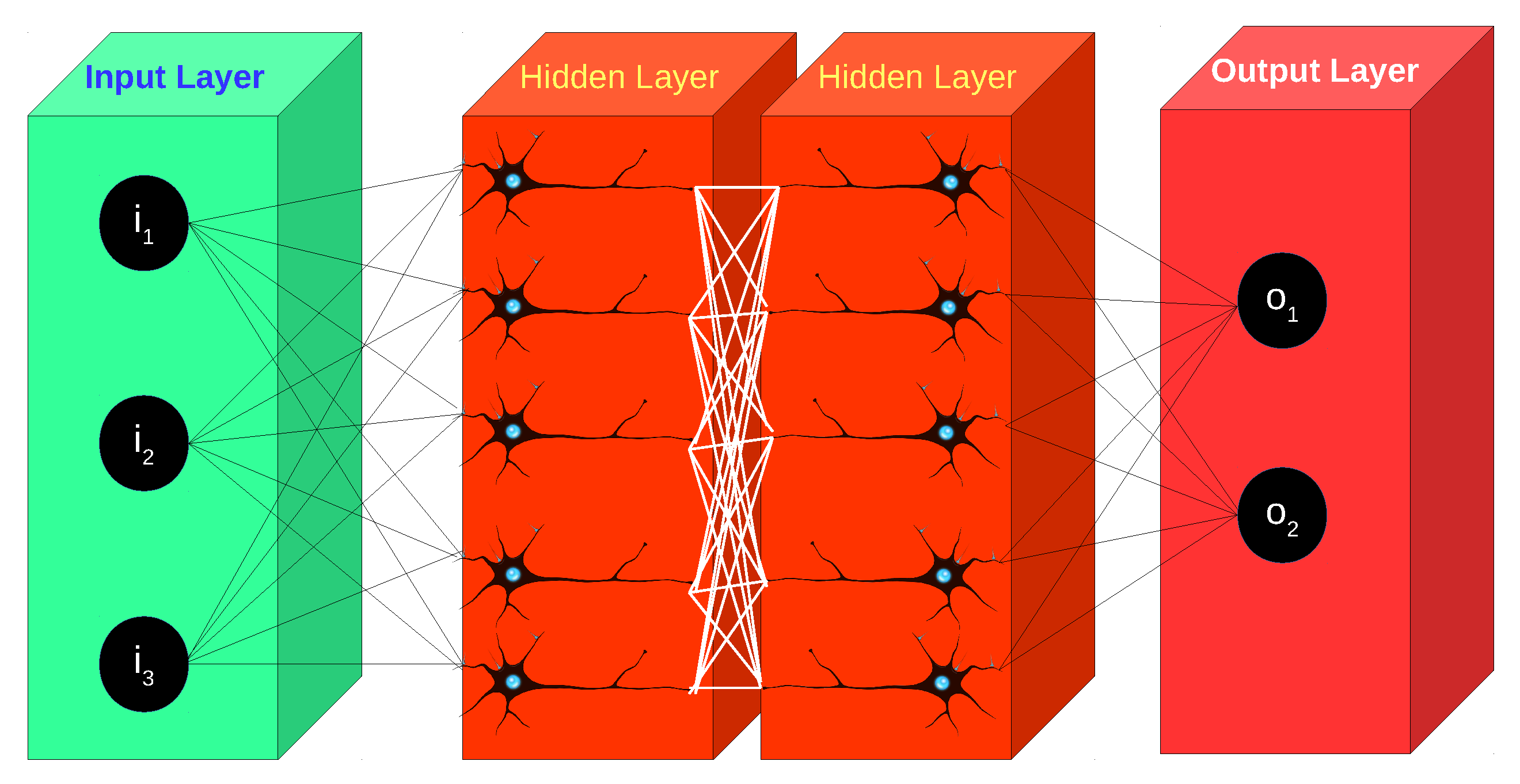
In Figure 2, we depict an example of an MLP architecture of two hidden layers with five neurons each, a three-dimensional input vector and a two-dimensional output vector.
Based on the magnitude of the error signal, defined as the difference between the actual output and the estimated output for an input signal, the network weights are adjusted to reduce the error. Once trained with a suitably representative training data, MLP can be applied to new and unseen input data. A scheme of the adopted MLP strategy is shown in Figure 3.
First, we identified the hourly inputs that are mostly correlated with leaf wetness. They could be resumed as follows:
- Air Temperature (°C): an increase/decrease can lead to a faster/slower evaporation of the water on the leaf surface,
- Relative Humidity (%): high humidity can cause the presence of dew on the leaf surface.
- Rainfall (mm): directly makes the leaf surface wet,
- Wind Speed (m/s): dries out the leaf surface,
- Solar Radiation (MJ/m2): one of the indicators of the behaviour of leaf wetness with respect to daily weather conditions (sunny, rainy, cloudy, etc...).
Three features have been added to the previous ones in order to correlate them with the temporal position and the geographical position of the leaf wetness sensors. These are:
- Date and hour converted to serial number using unix timestamps method,
- Latitude, Longitude in Decimals Degree,
- Altitude (m).
For each of the Trentino’s weather stations handled by the Edmund Mach Foundation, hourly data from 1 January of 2010 to 1 June of 2016, amounting to about 3 million samples for each kind of data, have been collected. Each value has been validated to remove lacking or invalid data and then they have been fed as input for different Artificial Neural Network configurations that are separately trained and validated. For instance, weather data has been validated by retaining it within a range of acceptable values depending on the type of the data—for example, the temperature limits have been arbitrarily chosen as −20 °C and 40 °C (this choice has been adopted by observing the historical records of minimum and maximum temperature values in Trentino region). If data is invalid or missing, all of the input data within that hour is discarded. Although such a step leads to a significant decrease in the amount of available data, it permits removing outliers, allowing a neural network to properly fit input data.
After having removed 600 h from the above dataset to test the achieved results, the network has been trained using the backpropagation algorithm [15] whose role is to minimize the error between target and estimated output.
3. Results
In this section, achieved results, experimental set-up and results validation are presented.
3.1. Experimental Set-Up and Dataset Description
Due to the relevance of leaf wetness on the risk infection evaluation model, it is crucial to extend the data where no sensors are available. Taking Trentino as a region of interest, the leaf sensor displacement map is shown in Figure 4.
As shown in the above image, there are zones where leaf wetness data is extended for numerous kilometres from a station to another, resulting in a low quality of risk evaluation for such zones. In order to show the weather heterogeneity of Trentino region, Figure 5 compares the Temperature, Humidity, Rainfall and Leaf wetness of the weather stations of Caldonazzo and Levico during 2016.
Figure 5 demonstrates how important differences of weather data could also be found for close weather stations (Caldonazzo and Levico have a geodesic distance of 4.60 km).
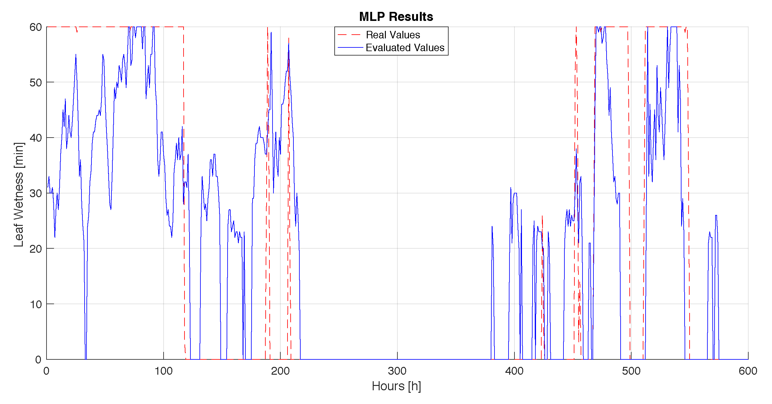
To resolve the leaf wetness geographical extension problem, we made use of an Artificial Neural Network that exploits weather data from the nearest weather station to evaluate leaf wetness in a specific orchard. The aim of this methodology in this application field is to give an advanced instrument to extract leaf wetness in a geographical position where no leaf wetness sensor is available. As explained previously, in order to achieve this, we utilize a Multi-Layer Perceptron Network (MLP) with the back-propagation algorithm to evaluate the data and the Mean Squared Error (MSE) as error analysis. Obtained results are reported in Figure 6 taking data from 600 h of the test dataset not used in the training process.
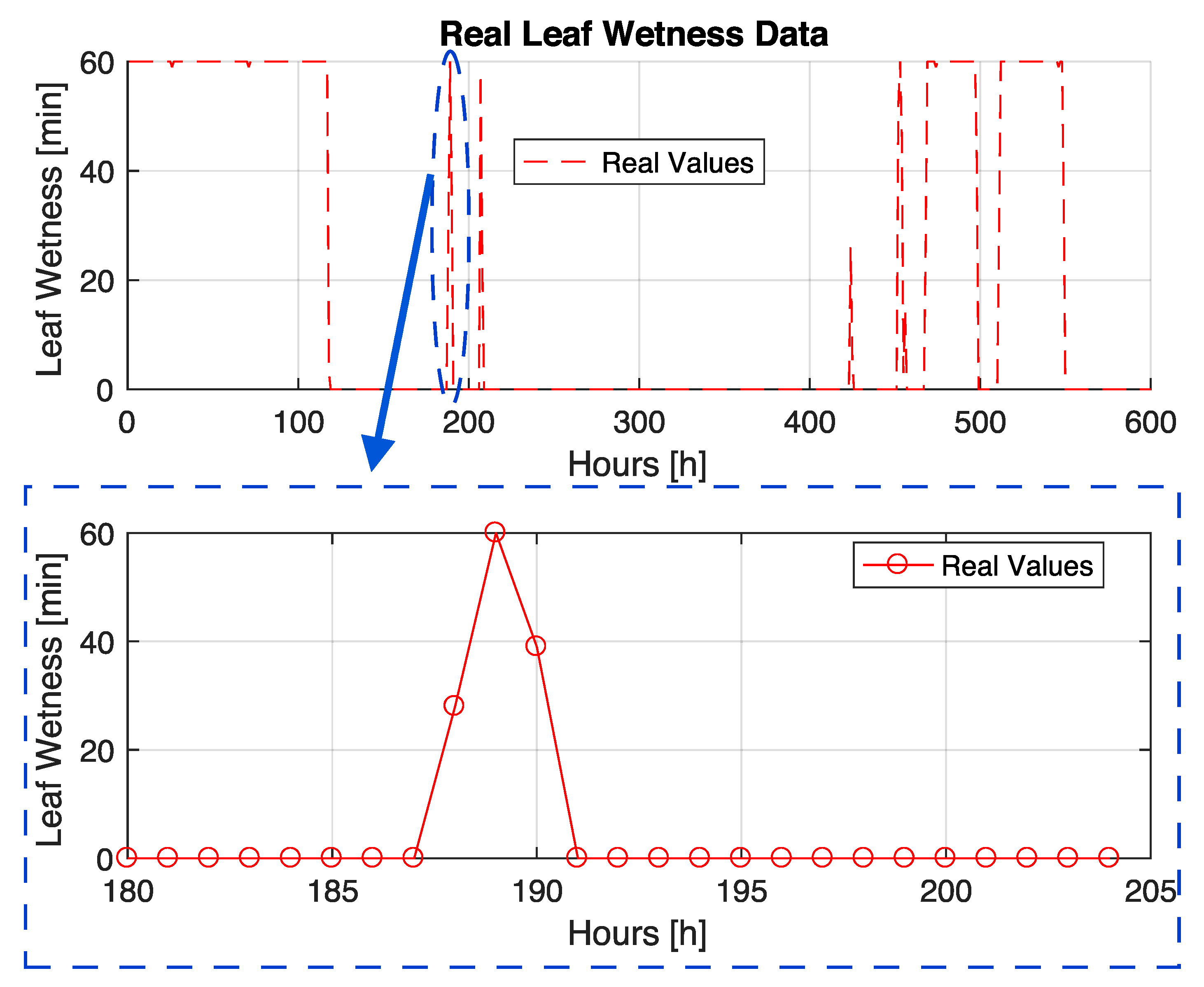
Due to the plot scale, by looking at the results shown above, the reader may be misled and may interpret real data of leaf wetness as binary data (0 min, 60 min). Instead, the leaf wetness data can assume all values between 0 and 60 min. For example, the plot from hour 180 to hour 204 of the above dataset is reported in Figure 7.
It is important to notice that the achieved results have to be evaluated in relation with risk infection computation. In fact, the MLP may overestimate or underestimate the leaf wetness data of one or more hour. However, what is important is that the overall amount of wetness does not lead to an incorrect potential risk evaluation. To better analyse the MLP output in the next subsections, some examples of risk evaluation analysis related to leaf wetness evaluation are reported.
3.2. Intra-Station Validation
Taking as the source of input the weather station placed in Segno (Latitude: 46.3048 [DD], Longitude: 11.076 [DD], Altitude: 525 m), the first test that was done is the comparison between the risk infection values computed using the leaf wetness data coming from the real sensor and its value computed using the MLP output at the geographical position of the weather station.
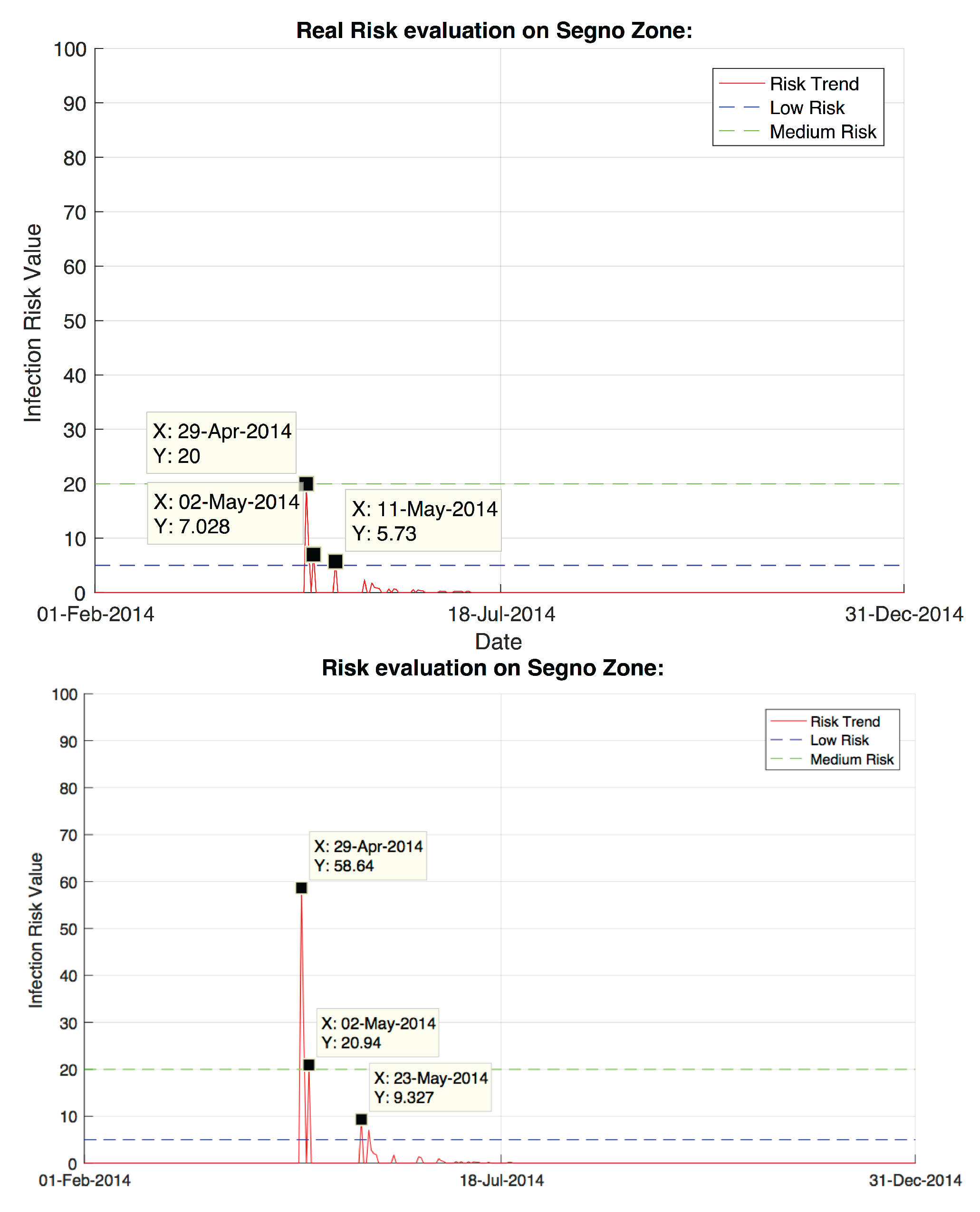
From Figure 8, it could be noticed that, using the MLP in this case, there is an overestimation of the risk for the first two dates of infection (29 April and 2 May) that leads to a translation of the third risk of infection from 11 May to 23 May. In this case, using MLP without having any previous knowledge of leaf wetness data, 66% of the total relevant infection event date has been detected; moreover, 100% of the most important events date have been correctly evaluated. It is important to underline the fact that the risk value has to be evaluated by considering the date of risk more than the risk value. In fact, whatever the risk infection value is, to avoid infection, the quantity of the preventive sprays is always the same and the only factor that makes a difference is the spray timing. Apple scab farmers have up to a maximum of 90 h to spray and prevent the infection. For what concerns risk infection value in the Apple Scab model, we have experimentally tuned two thresholds, namely, medium risk threshold and low risk threshold. Below the low risk threshold, there is a poor probability of contracting infection; thus, these values could be ignored; otherwise, the infection event has to be considered as a potentially damaging situation.
3.3. Cross-Station Validation
Due to the fact that the interest in leaf wetness data is subordinated to risk infection evaluation, the better way to evaluate the achieved results is in response to risk evaluation. Indeed, in order to have a complete validation of achieved results, we assume leaf wetness data acquired by the leaf wetness sensor as the most correct data available at a given geographical position. Therefore, the risk evaluation has been tested, taking as weather data the data coming from the nearest weather station to the one under examination as a source of input for the risk evaluation at the geographical position of the main weather station. To better explain the above illustrated method, two examples are reported in the following.
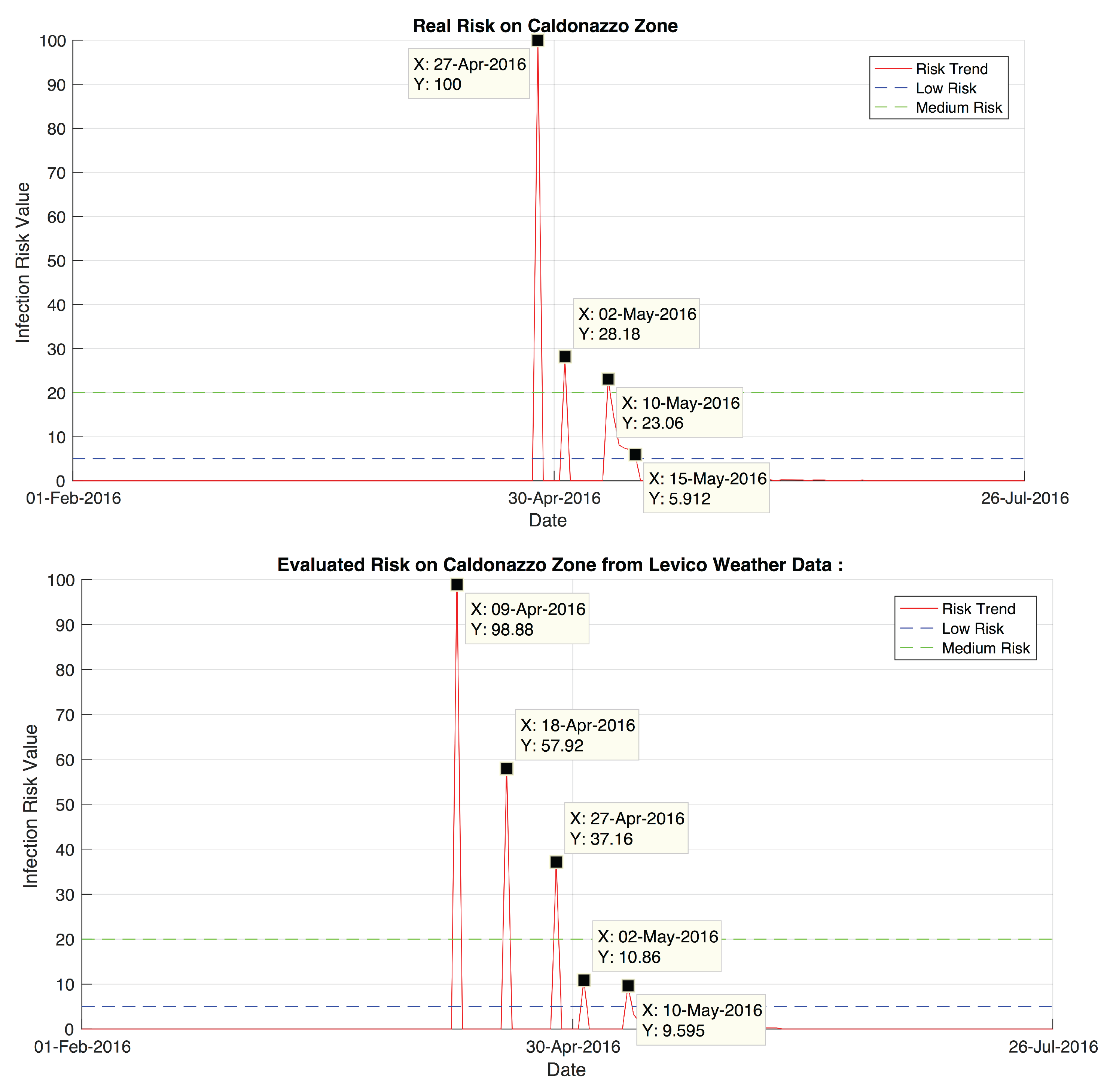
Table 1 and Figure 9 show the geographical position of Caldonazzo and Levico weather stations. Now, let us assume that the weather station of interest is the one in Caldonazzo. Thus, the comparison between the risk evaluation using data from Caldonazzo’s weather station and the risk evaluation using the weather data of Levico extending the leaf wetness on Caldonazzo’s position, in order to have its risk evaluation, is reported in the following (Example 4).
Figure 10 shows that using the MLP tends to introduce more risks of infection (9 April 2016 and 18 April 2016) with respect to the results obtained using the actual weather station data. Such overestimation of the number of the risks is not to be interpreted in a negative way. Indeed, as a matter of fact, for the farmer, it is safer to have an excess of treatments rather than missing a treatment. The important thing to notice is that the main infection events (the most important infection events to which more attention shall be paid are those that are due to the high population of Ascospores) (27 April 2016, 2 May 2016, 10 May 2016) are found by validating the leaf wetness estimation results. It is to notice that, in this case, the risk evaluation value for each of the main infection events is underestimated due to the addition of the infection events corresponding to 9 April 2016 and 18 April 2016. However, all of the main events are in the infection significant region (region above the low threshold risk), which leads to have a preventive treatment dose equal to the one that would be used in the actual risk evaluation (without the MLP).
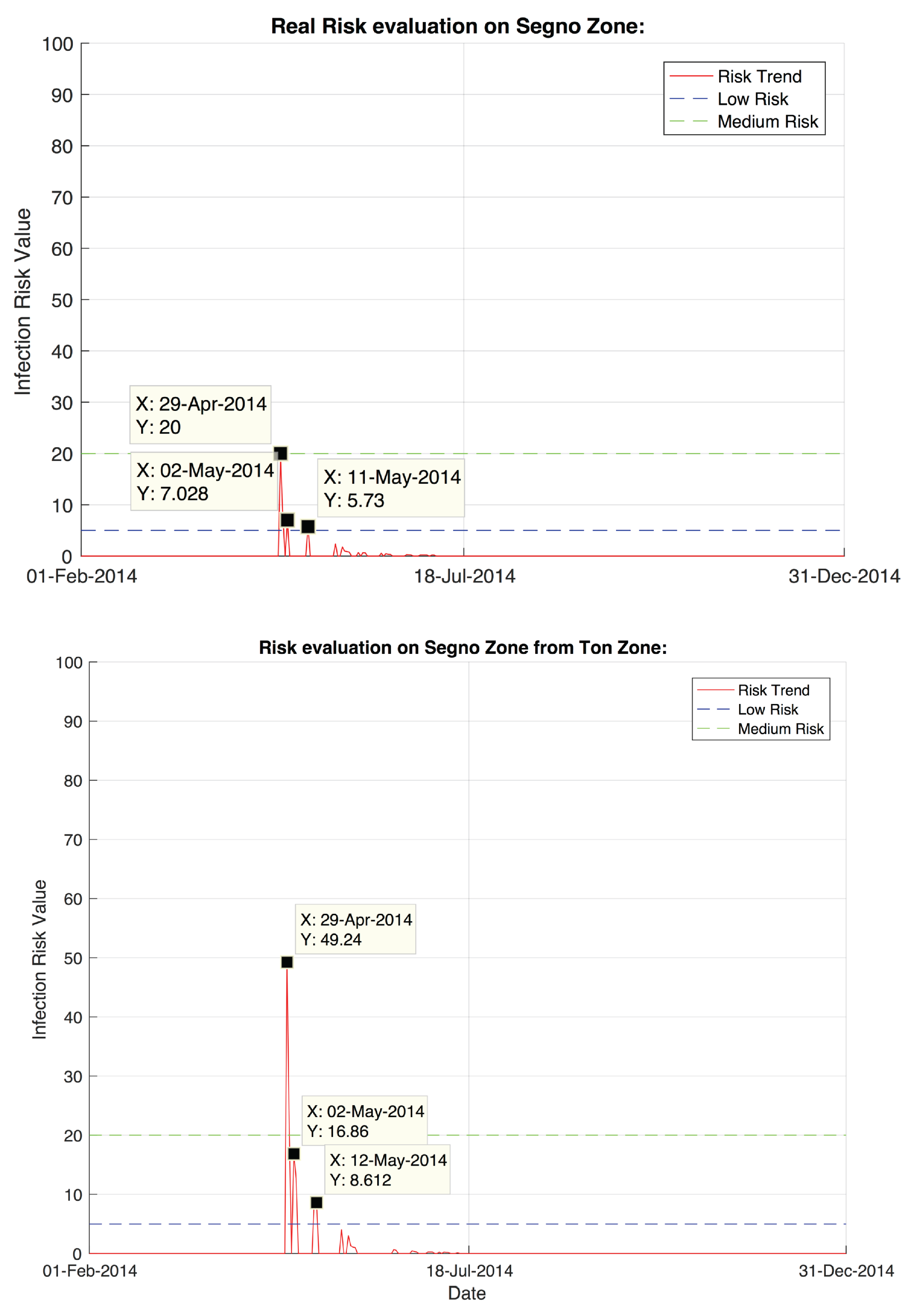
As another example, assume that the weather station of interest is the one in Segno, thus the comparison between the risk evaluation using data from Segno’s weather station and the risk evaluation using the weather data of Ton extending the leaf wetness to Segno’s position, in order to have its risk evaluation, is discussed below (Example 2).
Table 2 and Figure 11 report (Example 2) the geographical position of Caldonazzo and Levico weather stations.
Figure 12 shows that, in this case, using the MLP, the risk of infection dates are the same either using leaf wetness estimation with MLP or using sensor values. As it can be seen, the value of infection risk events are overestimated. An infection event date is valid until 90 h, which is the operational time for farmers to apply preventive measures. In this case, the difference between the infection event evaluated for the 11 May 2016 with the weather station data and the infection event evaluated for the 12 May 2016 using the MLP data could be considered the same infection event in the sense of spray timing to prevent infection.
For the role of completeness, in our validation analysis, the above experimental validation was applied to the all weather station dataset in order to have a full view of risk evaluation dependency from MLP output.
In the following, we report a table summarising the REE (Risk Evaluation Error) index for the year 2015. REE is an index which aims to give a quantitative feedback on the accuracy of the risk evaluation output using the MLP method. Basically, it is limited between 0 and 100 as a percentage, where 0 means that none of the major infection events have been found and 100 means that all of the significant infection events have been achieved. If there is no infection event for the whole season, REE returns −1; otherwise, if there is data lacking, which do not permit the usage of MLP (for example missing temperature or another input data for one or more hours), REE returns −2. First of all, the infection event using leaf wetness data coming from weather stations and from MLP are singularly evaluated and counted. After that, all of the infection events below the low risk threshold are rejected. Once only the most relevant infection events remain, each of the risk infection dates evaluated with MLP have looked for a corresponding date for the risk infection date evaluated with sensor value, considering that an error of a maximum of one day is admissible, in order to be safer. The number of found correspondences is then divided by the number of relevant infections found using the leaf wetness sensor data. Achieved results for REE evaluation using data from the same weather stations, as in the example reported in Section 3.2, are reported in Table 3.
3.4. Leaf Wetness Estimation without Sensor Coverage
In order to analyse the evaluation of risk in a region where no leaf wetness data is available, as an example, let us assume that the region of interest where the risk of infection has to be computed is near the weather station of San Michele all’Adige as shown in Figure 13 and Table 4. Let us label it San Michele External.
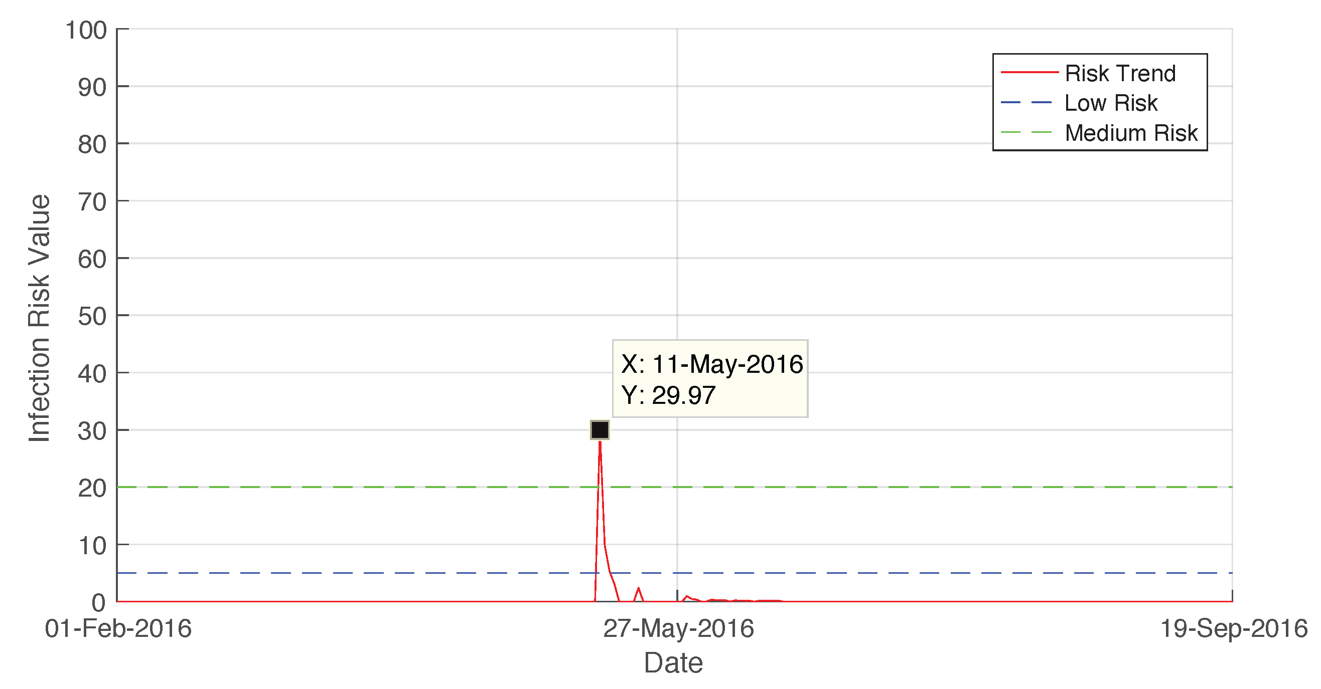
Without the leaf wetness estimation, the risk of this zone is considered to be equal to the one evaluated for San Michele at the position of the weather station, which is reported in Figure 14. Instead of using the leaf wetness extension shown below, it could be verified by looking at Figure 15: the infection risk evaluation is pretty different. In fact, it can be observed that the infection event in San Michele External on 11 May 2016 has a major potential risk value, and it has no risk of infection before this date.
Looking at the above examples, it could be shown that, in most cases, the critical infection events are found also with the leaf wetness evaluation and the difference between the risk infection values and the other infection dates are due primarily to the role of the other weather parameters (especially the temperature) as illustrated in Section 2. Nonetheless, it is important to specify that a greater value of infection risk index of first infection (that in literature are reported as the most relevant infections) compensates for the lack or the underestimation of a later infection risk event.
As far as the configuration of the MLP network is concerned, we have evaluated various architectures. The results reported so far correspond to the most efficient configuration, whose parameters are set as follows:
- Number of hidden layers: 2.
- Number of neurons per layer 1: 50.
- Number of neurons per layer 2: 20.
- Learning rate: 0.01.
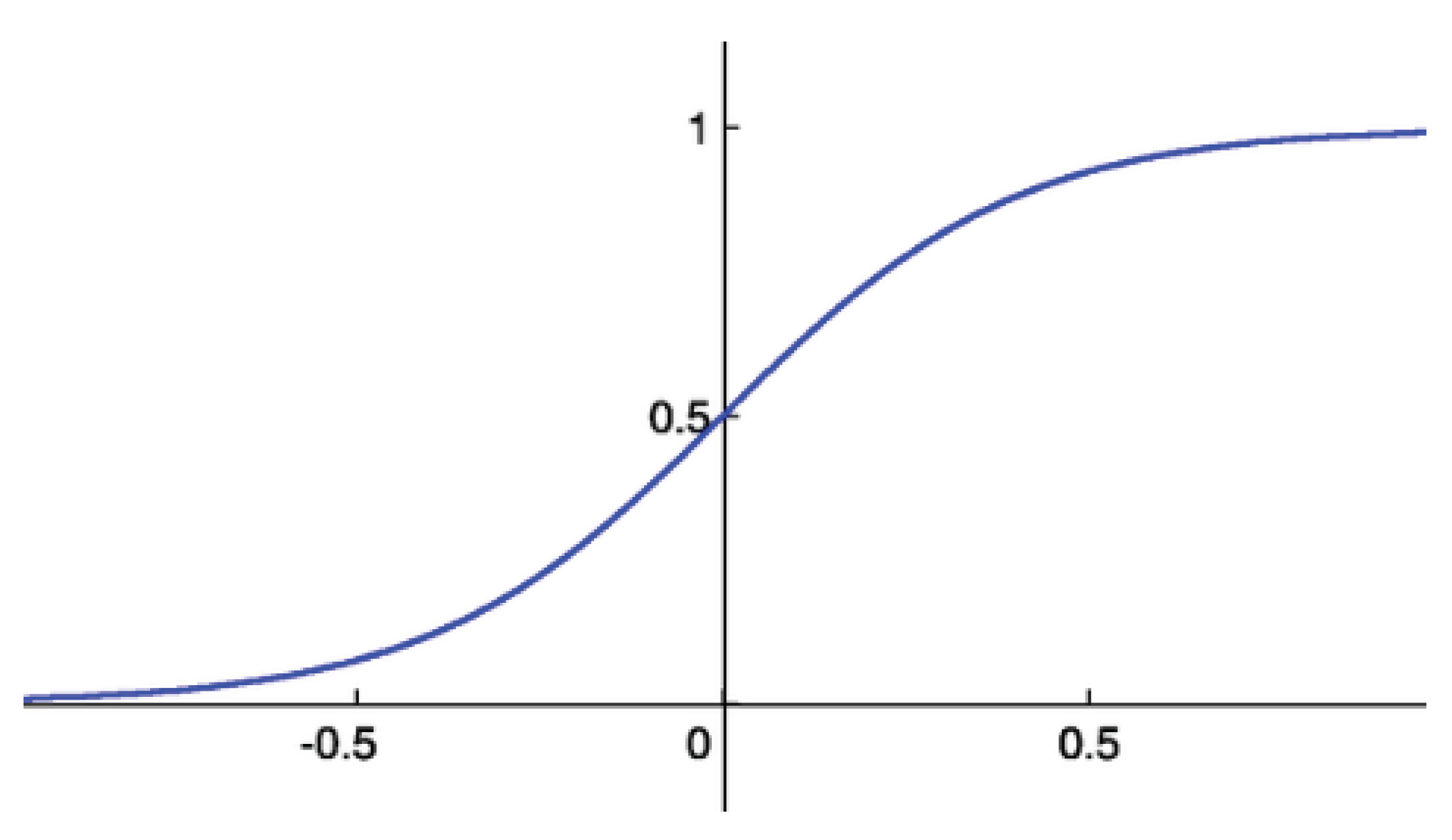
Activation function: Log-sigmoid (see Figure 16).
4. Conclusions
Apple Scab risk estimation based on models such as RimPro [16,17] and A-Scab strongly depends on (i) the position and on (ii) the quality of data coming from weather stations. Having the possibility of extending data or, in other terms, having more localised and thus more precise infection models within a given geographical region is extremely important for the farmers. The present work, besides providing an approach to estimating and generalising leaf wetness at any point across a given geographical region, is also useful for defining the best zone to place or replace a weather station in order to maximise its operative range. Moreover, it could be used as a forecast model for leaf wetness. Future works consist of training the neural network on other big data sets and to use the same approach to contextualize in a more precise way the temperature data through a geographical position, in order to better extend the risk infection model. As another future perspective, an index that quantifies the comparison of the evaluated and the real risk (Risk Evaluation Error), while also taking into account the washout of used spray, is under development. Thereupon, we aim to reduce spray events by optimising their efficiency and producing a more environmentally compatible and "green" cultivation, avoiding scab risk. Moreover, the intent of the whole project, from which this work is derived, is to give simple tools to the farmers that can help them make better prevision/decisions and choose the correct quantity of treatment product to spray.
Acknowledgments
This work is part of a project funded by the Autonomous Province of Trento under the provincial law 13/12/99 number 6 art. 5 to Metacortex S.r.l in collaboration with the University of Trento and the Edmund Mach Foundation. Authors would like to thank the Autonomous Province of Trento for the valuable opportunity, Mohamed Lamine Mekhalfi for the review of our work, Luisa Mattedi (Researcher at Edmund Mach Foundation), Gianbattista Toller, Fabio Zottele and Stefano Corradini (Researchers at the Geographic System Unit of the Edmund Mach Foundation) and Andrea Taddia (specialist at the Trentina’s company) for the collaboration and for the knowledge sharing.
Author Contributions
Alessandro Stella and Gennaro Caliendo conceived, designed and performed the experiments, analyzed the data and wrote the paper; Farid Melgani contributed with essential consultation and work revision; Nicola La Porta contributed with advice; Rino Goller and Maurizio Barazzuol subscribed and presented the Eye Scab Project to the Trentino Region.
Conflicts of Interest
The funding sponsors had no role in the design of the study; in the collection, analyses, or interpretation of data; in the writing of the manuscript, and in the decision to publish the results.
Abbreviations
The following abbreviations are used in this manuscript:
| ANN | Artificial Neural Network |
| LAI | Leaf Area Index |
| MLP | Multi-Layer Perceptron |
| PAT | Proportion of Ascospore that has been Trapped |
| UAV | Unmanned Aerial Vehicle |
References
- Mattedi, L.; Varner, M. Produzione Integrata Attraverso la Conoscenza delle Principali Malattie Fungine del Melo e della Vite; Arti Grafiche La Commerciale-Borgogno: Bolzano, Italy, 2000. [Google Scholar]
- Collier Arbor Care. Available online: http://www.collierarbor.com/probAppleScab.php (accessed on 12 June 2017).
- Passey, T.A.J.; Robinson, J.D.; Shaw, M.W.; Xu, X.-M. The relative importance of conidia and ascospores as primary inoculum of Venturia inaequalis in a southeast England orchard. Plant Pathol. 2017. [Google Scholar] [CrossRef]
- MacHardy, W.E. Apple Scab Biology, Epidemiology and Management; The Amercian Phytopathological Society: St. Paul, MN, USA, 1996; p. 545. [Google Scholar]
- Palmiter, D.H. Variability of Venturia inaequalis in cultural characters and host relations. Phytopathology 1932, 22, 21. [Google Scholar]
- Giosué, S.; Rossi, V.; Bugiani, R. A-scab (apple- scab), a simulation model for estimating risk of venturia inaequalis primary infections. In Proceedings of the EPPO Conference on Computer Aids for Plant Protection, Wageningen, The Netherlands, 17–19 October 2006; Volume 37, pp. 300–308. [Google Scholar]
- Zeggada, A.; Stella, A.; Caliendo, G.; Melgani, F.; Barazzuol, M.; La Porta, N.; Goller, R. Leaf Development Index Evaluation using Unmanned Aerial Vehicle Imagery for the Apple Scab Fight. In Proceedings of the IEEE International Geoscience and Remote Sensing Symposium (IGARSS 2017), Fort Worth, TX, USA, 23–28 July 2017. [Google Scholar]
- James, J.R.; Sutton, T.B. Environmental factors influencing pseudothecial development and ascospore maturation of Venturia inaequalis. Phytopathology 1982, 72, 1081–1085. [Google Scholar] [CrossRef]
- Rossi, V.; Ponti, I.; Marinelli, M.; Giosuè, S.; Buigiani, R. A new model estimating the seasonal pattern of air-borne ascospores of Venturia Inaequalis (Cooke) Wint. in relation to weather conditions. J. Plant Pathol. 2000, 82, 111–118. [Google Scholar]
- Stensvand, A.; Gadoury, D.M.; Amundsen, T.; Semb, L.; Seem, R.C. Ascospore release and infection of apple leaves by conidia and ascospores of Venturia inaequalis at low temperatures. Phytopathology 1997, 87, 1046–1053. [Google Scholar] [CrossRef] [PubMed]
- Gadoury, D.M.; MacHardy, W.E. Forecasting ascospore dose of Venturia inaequalis in commercial apple orchards. Phytopathology 1986, 76, 112–118. [Google Scholar] [CrossRef]
- Gardner, M.W.; Dorling, S.R. Artificial Neural Networks (the Multilayer Perceptron)—A Review of Applications in the Atmospheric Sciences. Atmos. Environ. 1998, 32, 2627–2636. [Google Scholar] [CrossRef]
- Hornik, K.; Stinchcombe, M.; White, H. Multilayer feedforward networks are universal approximators. Neura Netw. 1989, 2, 359–366. [Google Scholar] [CrossRef]
- Vali1, A.A.; Ramesht, M.H.; Mokarram, M. The Comparison of RBF and MLP Neural Networks Performance for the Estimation of Land Suitability. J. Environ. 2013, 2, 74–78. [Google Scholar]
- Beale, R.; Jackson, T. Neural Computing: An Introduction; Adam Hilger: Philadelphia, PA, USA, 1991. [Google Scholar]
- Cornell University. RIMpro as a Tool for Management of Apple Scab. Available online: https://blogs.cornell.edu/plantpathhvl/files/2016/01/RIMpro-as-a-Tool-for-Scab-Mgmt-15hf9bc.pdf (accessed on 12 June 2017).
- Trapman, M.C. Development and evaluation of a simulation model for ascosporeinfections of Venturia inaequalis. Nor. J. Agric. Sci. 1994, 17, 55–67. [Google Scholar]
Figure 1.
A-Scab main phases flowchart.
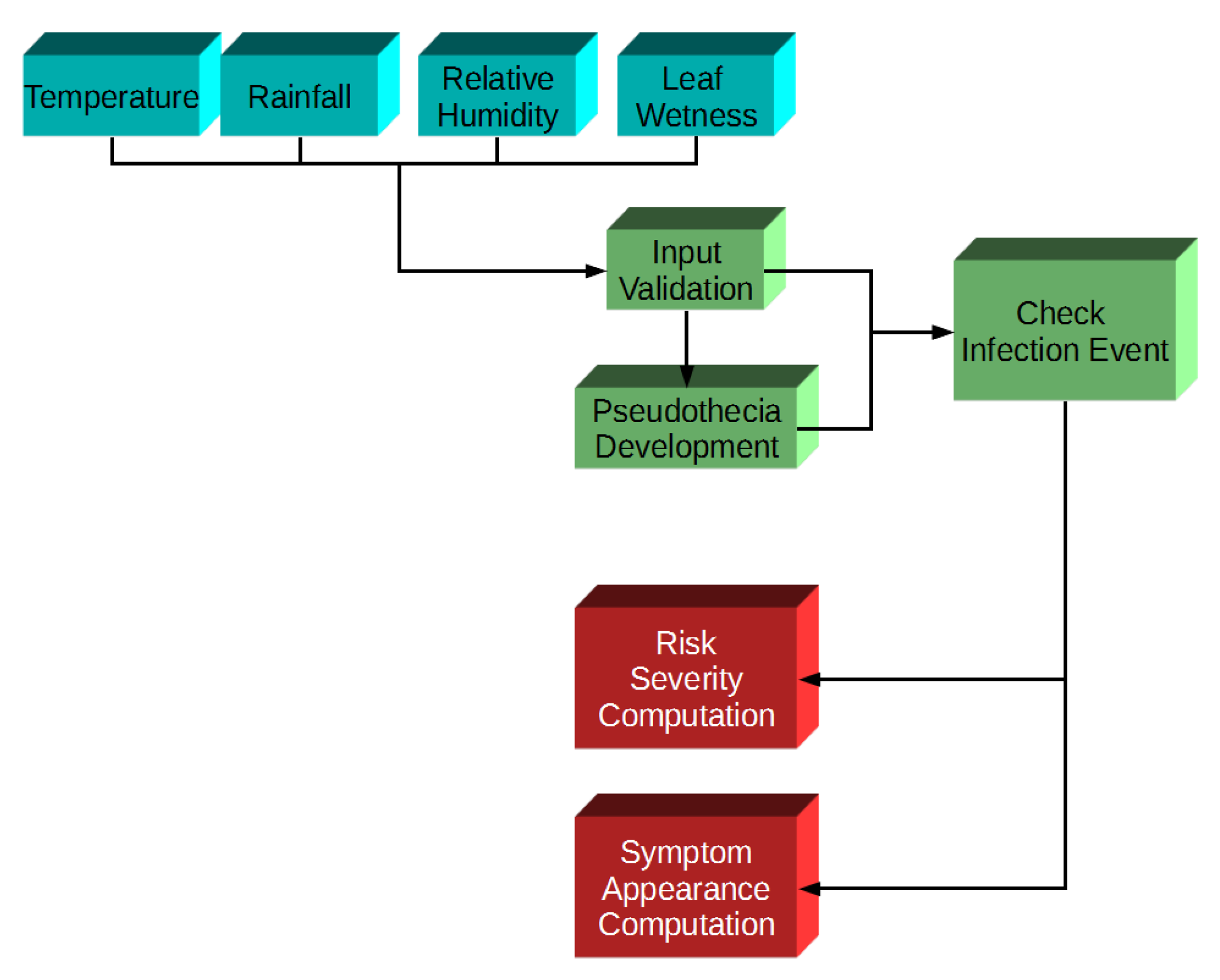
Figure 2.
Example of the Multi-Layer Perceptron neural network with two hidden layers, three inputs and two outputs.
Figure 2.
Example of the Multi-Layer Perceptron neural network with two hidden layers, three inputs and two outputs.

Figure 3.
Proposed Artificial Neural Network (ANN) for leaf wetness estimation.
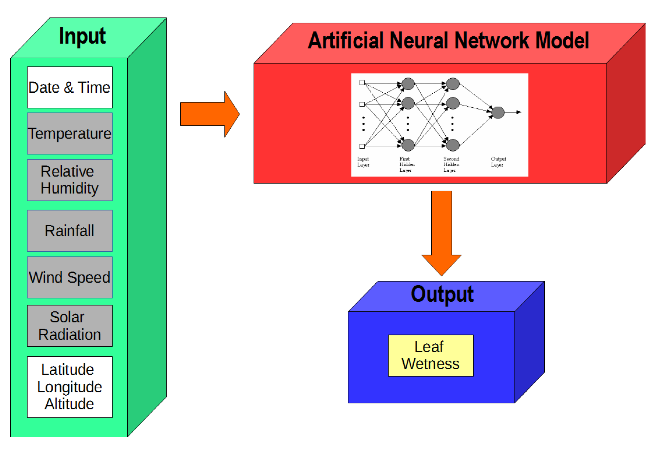
Figure 4.
Edmund Mach Foundation weather station positions in the Trentino region. The light blue circles represent the zones used in this paper as examples.
Figure 4.
Edmund Mach Foundation weather station positions in the Trentino region. The light blue circles represent the zones used in this paper as examples.
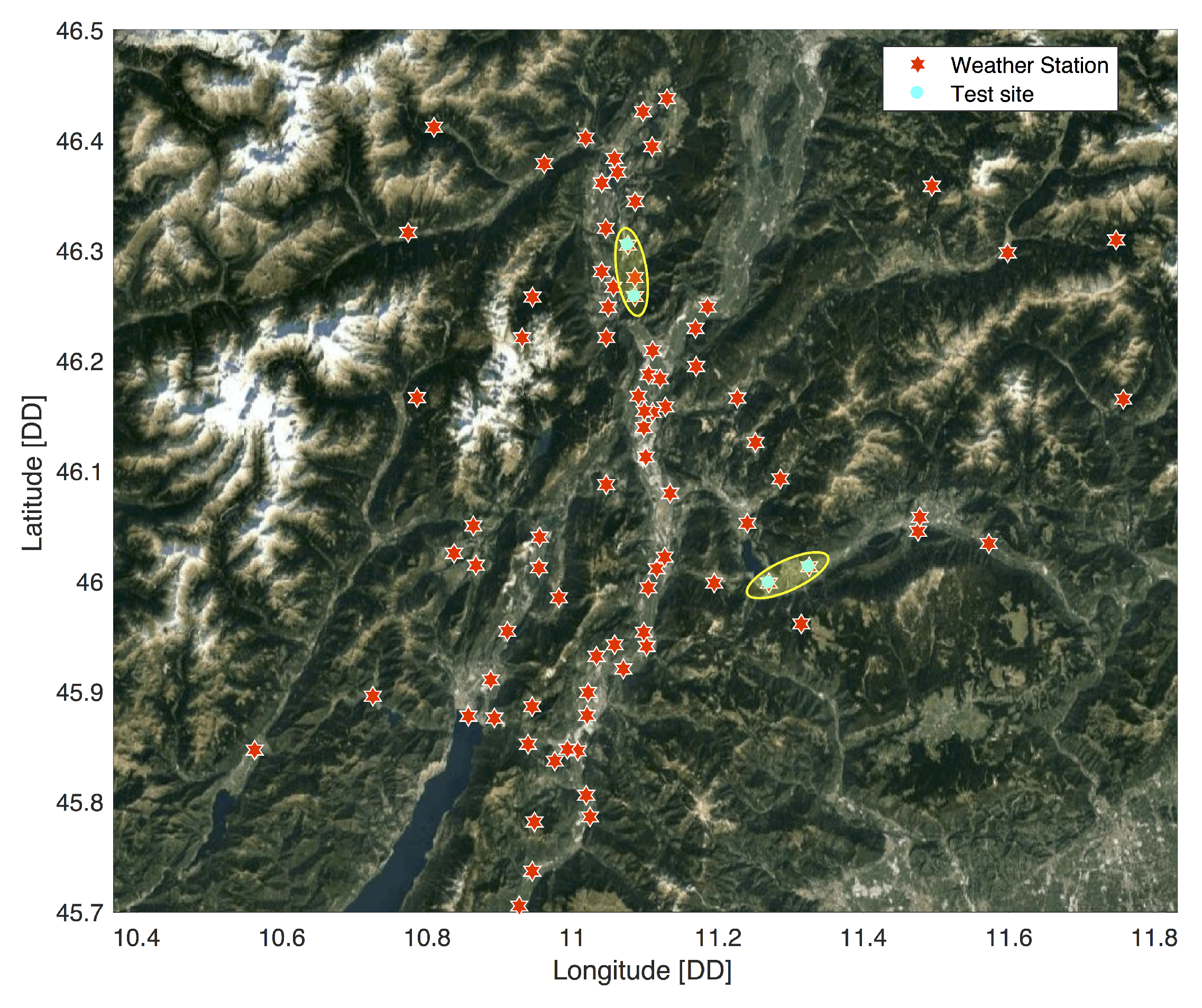
Figure 5.
Comparison between main weather data of Caldonazzo and Levico weather stations, from the 1 January 2016 to 26 July 2016. The red dashed line represents Levico’s weather data, and the blue line represents Caldonazzo’s weather data. Note that these two stations are only 4.6 km apart.
Figure 5.
Comparison between main weather data of Caldonazzo and Levico weather stations, from the 1 January 2016 to 26 July 2016. The red dashed line represents Levico’s weather data, and the blue line represents Caldonazzo’s weather data. Note that these two stations are only 4.6 km apart.

Figure 6.
Comparison between leaf wetness data acquired by sensors and values evaluated with the MLP neural network, correlation coefficient R = 0.75849.
Figure 6.
Comparison between leaf wetness data acquired by sensors and values evaluated with the MLP neural network, correlation coefficient R = 0.75849.

Figure 7.
Zoom in on real leaf wetness values between hour range [180, 204]. Red circles represent the hourly acquired leaf wetness value.
Figure 7.
Zoom in on real leaf wetness values between hour range [180, 204]. Red circles represent the hourly acquired leaf wetness value.

Figure 8.
Risk evaluation comparison; on the top, the risk evaluation for Segno’s zone using weather data of its own weather station; at the bottom, the risk evaluation for Segno’s zone using leaf wetness evaluated with the MLP.
Figure 8.
Risk evaluation comparison; on the top, the risk evaluation for Segno’s zone using weather data of its own weather station; at the bottom, the risk evaluation for Segno’s zone using leaf wetness evaluated with the MLP.

Figure 9.
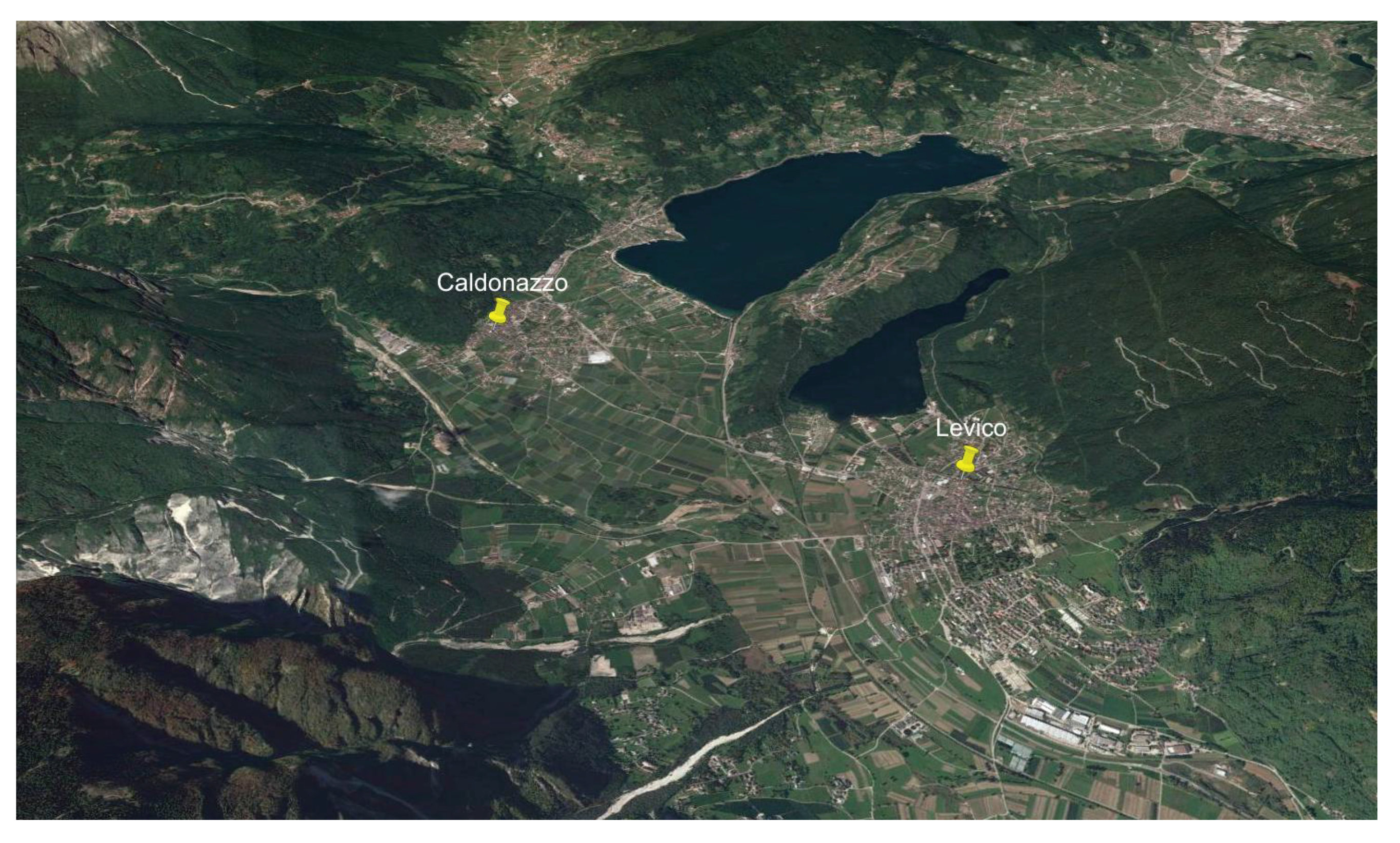
Caldonazzo and Levico geographical position view; geodesic distance of about 4.60 km.

Figure 10.
Risk evaluation comparison for Example 1: on the top, risk evaluation for Caldonazzo’s zone using weather data of its own weather station; at the bottom, risk evaluation for Caldonazzo’s zone using weather data of Levico’s weather station.
Figure 10.
Risk evaluation comparison for Example 1: on the top, risk evaluation for Caldonazzo’s zone using weather data of its own weather station; at the bottom, risk evaluation for Caldonazzo’s zone using weather data of Levico’s weather station.

Figure 11.
Segno and Ton geographical position view, geodesic distance of about 3.35 km.

Figure 12.
Risk evaluation comparison for Example 2: on top, risk evaluation for Segno’s zone using weather data of its own weather station; at the bottom, risk evaluation for Segno’s zone using weather data of Ton’s weather station.
Figure 12.
Risk evaluation comparison for Example 2: on top, risk evaluation for Segno’s zone using weather data of its own weather station; at the bottom, risk evaluation for Segno’s zone using weather data of Ton’s weather station.

Figure 13.
Geographical view of San Michele weather station (right pin) and San Michele External zone (left pin), where risk of infection has to be evaluated, geodesic distance of about 4.24 km.
Figure 13.
Geographical view of San Michele weather station (right pin) and San Michele External zone (left pin), where risk of infection has to be evaluated, geodesic distance of about 4.24 km.

Figure 14.
Risk of infection evaluated at San Michele without leaf wetness evaluation. For an infection model that does not use the MLP for leaf wetness extension, this risk coincides with the one for the San Michele External zone.
Figure 14.
Risk of infection evaluated at San Michele without leaf wetness evaluation. For an infection model that does not use the MLP for leaf wetness extension, this risk coincides with the one for the San Michele External zone.
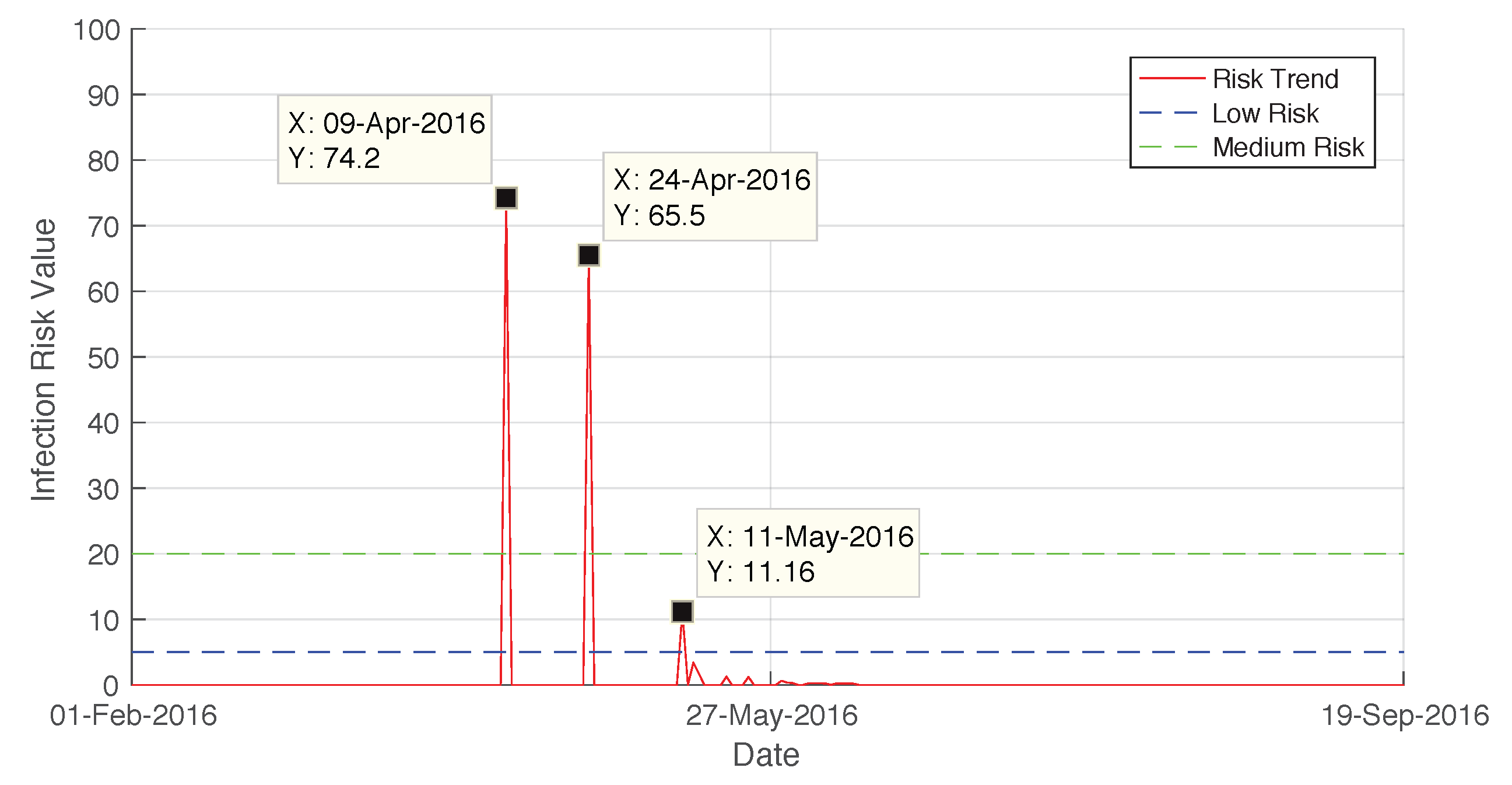
Figure 15.
Risk of infection evaluated at the San Michele External position using weather data coming from San Michele weather station data and extending the leaf wetness data using the MLP technique at the geographical position of San Michele External. This risk evaluation differs from the one acquired in San Michele.

Figure 16.
Log-sigmoid transfer function.

Table 1.
Geographical coordinates of the weather stations for Example 1.
| Weather Station | Latitude [DD] | Longitude [DD] | Altitude (m) |
|---|---|---|---|
| Caldonazzo | 45.99825 | 11.2699 | 461 |
| Levico | 46.01302 | 11.3253 | 449 |
Table 2.
Geographical coordinates of weather station for Example 2.
| Weather Station | Latitude [DD] | Longitude [DD] | Altitude (m) |
|---|---|---|---|
| Segno | 46.3048 | 11.076 | 525 |
| Ton | 46.258 | 11.0856 | 443 |
Table 3.
Risk Evaluation Error for each of the Edmund Mach Foundation weather stations in 2015. Risk Evaluation Error values of −1 means that no risk of infection has been computed, Risk Evaluation Error values of −2 correspond to missing weather values for Leaf Wetness evaluation.
Table 3.
Risk Evaluation Error for each of the Edmund Mach Foundation weather stations in 2015. Risk Evaluation Error values of −1 means that no risk of infection has been computed, Risk Evaluation Error values of −2 correspond to missing weather values for Leaf Wetness evaluation.
| Weather Station | REE Value (%) | Weather Station | REE Value (%) |
|---|---|---|---|
| Ala | 56 | Aldeno | −2 |
| Arco | 83 | Arsio | 83 |
| Avio | −2 | Banco Casez | −2 |
| Baselga di Piné | −2 | Besagno | 55 |
| Besenello | 67 | Bezzecca | −2 |
| Bleggio Superiore | −2 | Borgo Valsugana | 61 |
| Brancolino | −2 | Caldes | 66 |
| Caldonazzo | 87 | Cavedine | 52 |
| Cembra | −2 | Cles | −2 |
| Cognola | −2 | Coredo | −2 |
| Cunevo | −2 | Denno | 66 |
| Dercolo | −2 | Dro | 47 |
| Faedo | −2 | Fondo | −2 |
| Gardolo | 53 | Giovo | 69 |
| Lavazé | −2 | Lavis | 23 |
| Levico | −2 | Livo | 68 |
| Lomaso | −2 | Loppio | 83 |
| Malga Flavona | −2 | Mama di Avio | 66 |
| Marco | −2 | Maso Callianer | −2 |
| Mezzocorona Novali | 33 | Mezzocorona Piovi Veci | −1 |
| Mezzolombardo | 43 | Mori | 47 |
| Nago | −2 | Nanno | −2 |
| Nave San Rocco | −2 | Nomi | 87 |
| Ospedaletto | 74 | Paneveggio | −2 |
| Passo Vezzena | −2 | Pedersano | −2 |
| Pellizzano | −2 | Pergine | 59 |
| Pietramurata | 86 | Pinzolo Prà Rodont | −2 |
| Polsa | −2 | Predazzo | −2 |
| Pressano | 80 | Rabbi | −2 |
| Revo | 66 | Riva del Garda | −2 |
| Romagnano | −2 | Romeno | −2 |
| Ronzo Chienis | −2 | Rovere della Luna | 50 |
| Rovereto | −2 | San Michele all Adige | −2 |
| Sant Orsola | 60 | Sarche | |
| Savignano | −2 | Segno | 85 |
| Serravalle | 58 | Spormaggiore | 78 |
| Stenico | −2 | Storo | 83 |
| Telve | 72 | Terlago | 24 |
| Terzolas | −1 | Ton | 80 |
| Toss Castello | −2 | Trento Sud | −2 |
| Verla | 38 | Vigolo Vattaro | 76 |
| Volano | −2 | Zambana | 67 |
| Zortea | −2 |
Table 4.
Geographical coordinates of weather stations for Example 3.
| Weather Station | Latitude [DD] | Longitude [DD] | Altitude (m) |
|---|---|---|---|
| San Michele | 46.1835 | 11.12022 | 204 |
| San Michele External | 46.1964 | 11.17147 | 726 |
© 2017 by the authors. Licensee MDPI, Basel, Switzerland. This article is an open access article distributed under the terms and conditions of the Creative Commons Attribution (CC BY) license (http://creativecommons.org/licenses/by/4.0/).
Share and Cite
MDPI and ACS Style
Stella, A.; Caliendo, G.; Melgani, F.; Goller, R.; Barazzuol, M.; La Porta, N. Leaf Wetness Evaluation Using Artificial Neural Network for Improving Apple Scab Fight. Environments 2017, 4, 42. https://doi.org/10.3390/environments4020042
AMA Style
Stella A, Caliendo G, Melgani F, Goller R, Barazzuol M, La Porta N. Leaf Wetness Evaluation Using Artificial Neural Network for Improving Apple Scab Fight. Environments. 2017; 4(2):42. https://doi.org/10.3390/environments4020042
Chicago/Turabian StyleStella, Alessandro, Gennaro Caliendo, Farid Melgani, Rino Goller, Maurizio Barazzuol, and Nicola La Porta. 2017. "Leaf Wetness Evaluation Using Artificial Neural Network for Improving Apple Scab Fight" Environments 4, no. 2: 42. https://doi.org/10.3390/environments4020042
Note that from the first issue of 2016, this journal uses article numbers instead of page numbers. See further details here.