The Effect of Using a Geopedological Approach in Determining Land Quality Indicators, Land Degradation, and Development (Case Study: Caspian Sea Coast)

Abstract

This study addresses the escalating global concern surrounding land degradation (LD) and its far-reaching implications on water and nutrient availability, as well as on human health and well-being. Focused on the southeastern Caspian Sea region, this research employs a novel remote sensing geo-pedological methodology to comprehensively assess soil and land quality dynamics, particularly influenced by salts, and investigates the intricate relationship between LD and soil development. The study area, marked by a susceptibility to seawater level fluctuations and diverse landforms (lagoons, barriers, and coastal plains) offers a unique opportunity for geopedologic analysis. Utilizing particle size distribution data, six distinct landforms are identified, providing insights into the region’s complex sedimentary history. A soil quality assessment is conducted remotely through the calculation of two indexes—the Integrated Quality Index (IQI) and the Nemoro Quality Index (NQI)—employing both Total Data Set (TDS) and Minimum Data Set (MDS) methodologies. The investigation highlights the role of soluble salts in shaping soil quality, thereby influencing LD and development dynamics. The differentiation of landforms significantly enhances classification accuracy, providing a more nuanced understanding of the multifaceted factors governing LD. The study’s implications extend beyond the southeastern Caspian Sea region, and demonstrate that the potential for incorporating a geopedologic approach when assessing soil and land quality dynamics in arid regions globally. Our analytic approach can inform policymakers and land managers when making decisions to combat LD and foster sustainable land development. This research also contributes towards advancing knowledge in geopedology by providing a robust foundation for future studies aimed at enhancing land management practices in the face of ongoing environmental challenges.

1. Introduction

Land degradation (LD) exerts adverse effects on water quality and nutrient availability [1] for approximately 3.2 billion people and about 40% of agricultural land [2]. Combatting LD is a prominent benchmark for the United Nations Sustainable Development Goals (for 2030) [3]. The term “LD” is variably defined, with each interpretation highlighting distinct dimensions of reduced land quality [4]. The spread of LD significantly impacts human health and community welfare, specifically in developing countries [5,6,7]. The continual degradation of agricultural lands is expected to persist in the coming decades, driven by resource scarcity, and this pressure compels farmers to exploit cultivated land for their livelihoods [1,8].

Global efforts since 2010 have suggested innovative interventions to arrest LD and rehabilitate compromised land at the regional and global scales. The Sustainable Development Goals (SDGs), adopted by 193 nations in September 2015, came into effect in January 2016, with projections to shape economic, social, and environmental policies by 2030 [4]; many potentially lessening LD. The United Nation’s SDGs set a clear objective to reduce desertification by 2030, encompassing sustainable forest management, combating desertification, and safeguarding and promoting sustainable terrestrial ecosystems, as well as reversing LD and halting biodiversity loss [9].

Drylands in arid regions presently occupy 41.3% of the global land area and are projected to grow by 11–23% by the century’s close [10]. Although predominantly located in developing countries, these lands have significantly expanded [11]. Given that both agricultural and degraded lands are influenced by natural and socioeconomic factors, with the interplay of land use and cover [10,11], the management of lands in arid and semiarid regions is paramount for global change research. Thus, studying such lands in arid and semiarid regions is one of the primary necessities of global change research.

Implementing the United Nations Convention to Combat Desertification (UNCCD) [12] to monitor and evaluate LD and monitoring management program performance requires approved scientific and practical methods. A lack of adequate and coherent monitoring and evaluation in the past has been suggested as a main limitation in combatting desertification, and implementing efficient programs requires careful analysis, the presentation of a clear scientific concept of processes, and LD incentives [13]. Detailed landscape information from a study area is needed to avoid, mitigate, and control LD.

This study aims to determine the soil and land quality of the southeastern Caspian Sea region using land quality models and methods and to investigate the relationship between LD and development using a geopedologic approach. Central to a geopedologic approach is an evaluation of LD and other geohazards [14]. A geopedologic approach integrates the disciplines of geomorphology (genesis of landforms) and pedology (genesis of soils) to understand the relationships between landforms and soils. This approach examines the influence of geologic and geo-morphic factors on soil development, classification, and distribution [14,15]. Most studies utilizing a geopedologic approach have been based solely on the characteristics of the topography and surface geometry of the earth, and there is not enough focus on flat and coastal lands and the process of degradation or development of such lands. The present study significantly contributes to existing research on LD and geohazard evaluation through the innovative application of a geopedologic approach. Unlike previous studies, which often focused on the characteristics of topography and surface geometry, this research specifically addresses flat and coastal lands, investigating the processes of degradation and development in these areas using inherent and dynamic soil properties. The given study area can be considered as a plain (less than 2% general slip), utilizing a geopedological approach can provide a comprehensive understanding of the intricate relationships between landforms and soils in the southeastern Caspian Sea region. This approach not only enhances our ability to assess land quality accurately but also contributes valuable insights for effective land management strategies. The study aligns with global initiatives, such as the Sustainable Development Goals (SDGs) and the United Nations Convention to Combat Desertification (UNCCD), emphasizing the importance of addressing LD for sustainable development. Through this research, the authors seek to fill gaps in current knowledge, laying the groundwork for improved monitoring, evaluation, and management of LD in arid and semiarid regions [9].

The present study addresses the environmental concern of LD and its impact on soil and human health and well-being in the southeastern coastal areas of the Caspian Sea. Using a novel geopedologic method, the research comprehensively evaluates soil and land quality dynamics influenced by salts in an area susceptible to seawater fluctuations and in which these sea water fluctuations have brought about the creation of diverse landforms, as confirmed by the authors of the present study. Identifying six distinct landforms through PSD granulometric curves and DEM information was supposed to enhance accuracy of land quality classifications [14]. Soil quality assessment, using both the Integrated Quality Index (IQI) and the Nemoro Quality Index (NQI), emphasizes the roles of soluble salts in soil quality and LD dynamics [9,13]. On the plus side, the present study demonstrates the potential of geopedologic approach to assess soil and land quality dynamics in global scales, with implications for informing land managers and policymakers against LD and fostering sustainable land development. Contributing the advancement of geopedologic knowledge for future studies will improve land management practices among environmental issues.

2. Materials and Methods

2.1. Study Area

The southeastern Caspian Sea region was selected as the study area given that it is driven by its unique characteristics and current LD challenges. This region is particularly susceptible to seawater level fluctuations and different coastal landforms, including lagoons, barriers, and coastal plains. Such distinct environmental attributes create a unique opportunity for geopedologic analysis because researchers can investigate the intricate relationship between LD and soil development in a complex coastal setting (Figure 1). Furthermore, the significance of the southeastern Caspian Sea region goes beyond its distinctive geologic and geomorphic features. The region plays a crucial function in the context of environmental challenges, due to its susceptibility to LD. Investigating the dynamics of land and soil quality in selected areas has broader implications for addressing similar issues in arid and semiarid regions worldwide. The extent of the study area is about 480 km² (20 km × 24 km) located on the southeastern coast of the Caspian Sea (54°21′10″ E, 37°18′57″ N:53°54′58″ E, 37°18′57″ N) (Figure 1b). At the time of this study (Summer 2019), the shoreline of the Caspian Sea in the study area was −27 m below mean sea level [15]. The study area’s mean annual temperature is 17.6 °C (hottest month: August, mean 27.8 °C and coldest month: January mean 7.7 °C), the mean annual precipitation is 250–550 mm (ap-proximately 350 mm in the study area) [16]. The southeastern Caspian Sea coast has a semi-arid climate, with a mean annual precipitation of 250–550 mm (approximately 350 mm in the study area) [15,16,17].

The coastal plain in the study area is affected by sediments from three major rivers (the Gorgan, Atrak, and Qarah Soo), which pass through aeolian materials susceptible to erosion. The gradients of these rivers flatten abruptly upon entering the plains, and the speed of the water flow decreases [15,16]. The rivers contain large quantities of suspended material which are deposited upon entering the lagoons and marshy environments and are eventually deposited as layers with a particular size distribution (mainly silt) [17]. Depending on the intensity of inlet currents and the turbulent or stationery nature of the sedimentary environments, the deposition sequence and particle size distribution vary widely. Topography of coastal regions, ocean currents, waves, and rapid sea-level changes are key factors controlling coastal geomorphology [16]. The coastal features of the Caspian Sea coast indicate that the morphology before the present state has formed barriers, barrier flats, lagoons, lagoon relict, lagoonal deposits, and coastal plains. The separation of landform units in flat coastal areas without strong physiographic differences limits precise landform classification. Therefore, in addition to satellite imagery and information derived from digital elevation model (DEM) (Figure 2) analysis, granulometry information (i.e., PSD) has been used [18] to identify soils in sedimentary environments (Figure 3).

2.2. Landform Definitions

Six previously defined landforms were used to assess soil quality [18,19,20]:

Relict (adjective): Pertaining to surface landscape features, e.g., landforms, geomorphic surfaces, and paleosols that have never been buried and yet are predominantly products of past environments.

Lagoonal deposit: Sediments transported and deposited by wind, currents, and storm wash over on the various types of sand, silt and clay in the relatively low-energy, brackish to saline, shallow waters of a lagoon.

Lagoon [coast]: A shallow stretch of salty or brackish water, partly or completely separated from a sea or lake by an offshore reef, barrier island, sandbank, or spit. [Relict landform] A nearly level, filled trough or depression behind the longshore bar on a barrier beach and built by a receding pluvial or glacial lake. Compare—sewage lagoon.

Barrier flat: A relatively flat, low-lying area, commonly including pools of water, separating the exposed or seaward edge of a barrier beach or barrier island from the lagoon behind it. An assemblage of both deflation flats left behind migrating dunes and/or storm wash over sediments; may be either barren or vegetated.

Barrier: Something (such as a fence or natural obstacle) that prevents or blocks movement from one place to another or a physical object that blocks the way.

Coastal plain: A low, generally broad, plain that has, as its margin, an oceanic shore and its strata are horizontal or gently sloping toward the water; generally represents a strip of recently pro-graded or emerged sea floor, e.g., the coastal plain of the southeastern U.S. which extends for 3000 km from New Jersey to Texas [19,20]. Since, in the present study, coastal landforms have already been detected through internal soil properties rather than external soil geometry and soil external properties [18], it should be mentioned that understanding how each landform affects land and soil quality is essential for a comprehensive analysis. For example, typically, lagoons are shallow/coastal water bodies which are separated from the sea by barriers, or coral reefs. These water bodies can affect soil and land quality by affecting the water table, soil salinity, and deposited sediment. Soil quality may be affected by the periodic saltwater pro/retrogradation, influencing nutrient availability and biochemical properties. Barriers affect the quality of the soil due to the type of sediment and vegetation cover, influencing fertility and stability. Coastal plains can contribute to land and soil quality through depositional situations and the availability of water fluxes [19].

To determine soil/land quality indexes, various physicochemical measurements were performed using standard methods as follows: the assessment of pH and electrical conductivity (EC) in soil paste extracts [21], of calcium carbonate equivalents through calcimetry [22], and analysis of anions (CO₃²⁻, HCO₃⁻, Cl⁻ using titration and SO₄²⁻ via the acetone method). Additionally, cations (Ca²⁺ and Mg²⁺ by calcimetry, and Na⁺ and K⁺ by flame photometry) [22], sand, silt, clay, and SP, were also analyzed using standard procedures (methods of soil analysis, physical methods) [23], and determination of soil organic carbon (SOM) [24].

As shown in Figure 1b, 140 sampling points were selected from 7 rows, with each row containing 20 points (because of the paludal situation, four points had been lost from the last row). The reason for selecting a gridded sampling pattern was to cover all soil physicochemical changes along the shoreline to 20 km toward the east. On the other hand, to investigate soil quality indexes in tiny coastal landforms, using these kind of sampling points allows more samples from each landform to be used.

Figure 4 shows the pro/retrogradation of Caspian Sea water in the last 45 years (1975–2020) and the resulting changes in coastal landforms. As shown in Figure 2, from 1975 to 2000, seawater progradation is observed, which causes the formation of a lagoon, and a seawater retrogradation movement is detected from 2000 to 2020. According to Figure 2, most of the development and agricultural activities have occurred in the study area during the last five years (2015–2020), affecting the soil and land quality in this area.

An Integrated Quality Index (IQI) and Nemoro Quality Index (NQI) are calculated using Equations (1) and (2) according to two different approaches: a total data set (TDS) encompassing all study data and a minimum data set (MDS). Per Equation (1), the Integrated Quality Index (IQI) is obtained from the sum of the product of the weight of each attribute and the score of that attribute [25].

$$\mathrm{I}\mathrm{Q}\mathrm{I}=\sum _{\mathrm{i}=1}^{\mathrm{n}}{\mathrm{W}}_{\mathrm{i}}.{\mathrm{N}}_{\mathrm{i}}$$

(1)

Variable W_i is the weight assigned to each soil property, N_i is the score given to each property, and n is the number of properties used [26,27]. In Equation (2), the Nemoro Quality Indicators (NQI) are obtained based on the minimum and average of each feature.

$$\mathrm{N}\mathrm{Q}\mathrm{I}=\sqrt{\frac{{\mathrm{P}}_{\mathrm{a}\mathrm{v}\mathrm{e}.}^2+{\mathrm{P}}_{\mathrm{m}\mathrm{i}\mathrm{n}.}^2}{2}}\times \frac{\mathrm{n}-1}{\mathrm{n}}$$

(2)

Variable P_ave. is the average score assigned to the selected features in each soil sample, P_min. is the minimum score among the selected features for each sample, and n is the number of desired features [3,28]. Each indicator was determined for each soil sample using two sets of characteristics affecting soil quality, including TDS and MDS. Four general indicators were thus evaluated for each soil sample: IQI_MDS, IQI_TDS, NQI_MDS, and NQI_TDS.

Statistical analyses, including PCA, Eigenvalues, and general statistics, were performed using SPSS V26 (SPSS Inc., Chicago, IL, USA), and maps were prepared and extracted by ArcMap V10.6.1 (ESRI, Redlands, CA, USA). The geopedologic approach subdivided the study region into distinct smaller areas. This approach enables the categorization of soil and land qualities, providing a more nuanced understanding compared to treating the entire study area as a uniform plain.

3. Results and Discussion

3.1. Identification of Coastal Landforms

These analyses identified six distinct coastal landforms, including: barriers, barrier flats, lagoons, lagoon relict, and lagoonal deposits, and coastal plains have been identified using spatial configurations of contour lines extracted from digital elevation model (DEM) and particle size distribution (PSD) data. Understanding and classifying these landforms provide essential insights into the geomorphologic features of the study area [18].

PCA analysis with cumulative eigenvalues (

Table 1. Results of principal component analysis (PCA) in distinguished landforms. Bolded values are indicators which obtained weighted loading values within a 10% range of the highest weighted loading within each PCs.

Landforms	Lagoon Relict						Lagoon Deposit						Present Lagoon
Components	PC1	PC2	PC3	PC4	PC5	PC6	PC1	PC2	PC3	PC4	PC5	PC6	PC1	PC2	PC3	PC4	PC5	PC6
Total	6.81	3.92	2.3	1.87	1.55	1.35	7.98	2.82	2.5	1.81	1.18	1.04	5.76	4.25	2.71	2.46	2	1.47
% of Variance	32.45	18.65	10.93	8.9	7.38	6.43	37.99	13.4	11.89	8.63	5.59	4.94	27.44	20.22	12.88	11.71	9.51	6.99
Cumulative %	32.45	51.09	62.03	70.93	78.31	84.73	37.99	51.39	63.29	71.92	77.51	82.45	27.44	47.66	60.54	72.25	81.75	88.74
SOM	−0.34	−0.53	−0.31	−0.53	0.13	−0.14	−0.36	−0.09	0.27	−0.08	0.19	0.69	−0.15	−0.11	0.46	0.27	0.07	0.7
CaCO3	−0.50	0.69	−0.08	0.27	−0.12	0.24	0.73	−0.53	−0.14	−0.21	0.06	−0.21	0.54	−0.45	0.21	0.1	0.59	−0.13
SP	−0.43	0.08	0.17	0.34	0.12	−0.04	−0.67	0.13	0.5	−0.17	0.26	−0.10	0.48	−0.01	−0.09	0.46	0.44	−0.08
EC	0.91	−0.11	0	−0.13	0.31	−0.05	0.97	−0.06	−0.02	0.03	0	0.07	0.64	0.08	−0.48	0.12	0.33	0.27
pH	0.69	−0.29	−0.23	0.18	−0.48	−0.25	0.68	−0.39	−0.22	−0.19	0.36	−0.06	0.38	−0.60	0.15	0.17	0.01	0.55
Sand	−0.33	−0.54	0.52	−0.14	−0.08	0.26	0.41	0.28	0.61	0.28	0.13	−0.07	−0.25	−0.52	−0.48	−0.58	0.22	0.07
Silt	0.3	0.55	−0.04	−0.62	−0.33	0.21	0.52	0.4	−0.42	−0.15	0.45	0.1	0.3	0.62	0.19	0.52	−0.41	−0.09
Clay	−0.06	−0.17	−0.33	0.72	0.38	−0.40	−0.67	−0.50	−0.02	−0.04	−0.44	−0.04	−0.07	−0.15	0.76	0.25	0.42	0.04
Na+	0.95	0.01	0.03	0.02	0.22	0.14	0.78	−0.01	0.48	0.06	0.06	−0.07	0.83	−0.01	0.36	−0.14	−0.35	0.08
K+	0.84	0.4	−0.16	0.01	0.02	0.07	0.76	0.27	0.3	0.11	0	0.35	0.85	0.11	0.1	0.09	−0.12	−0.17
Ca2+	−0.40	0.29	−0.67	0.14	0.02	0.34	0.49	0.43	−0.36	0.33	−0.28	0.02	0.17	−0.20	−0.35	0.81	−0.21	−0.14
Mg2+	0.47	−0.13	0.22	0.1	0.52	0.63	0.54	0.41	−0.34	0.5	−0.23	0.05	0.65	0.44	−0.46	−0.10	−0.23	0.28
Cl−	0.92	−0.08	−0.05	−0.07	0.32	0.05	0.94	0.07	0.05	−0.04	0	0.17	0.79	0.05	−0.32	−0.03	0.23	0.27
CO32−	−0.59	0.08	−0.25	0.1	0.29	0.25	−0.15	0.71	−0.17	−0.30	0.09	−0.30	0.5	0.68	−0.22	0.06	0.39	0.05
HCO3−	−0.10	0.9	−0.13	−0.12	0.22	−0.05	−0.57	0.29	−0.03	−0.47	0.02	0.32	−0.19	−0.49	−0.39	0.5	−0.51	0.18
SO42−	0.58	0.23	0.36	0.42	−0.27	0.21	0.78	−0.26	−0.14	−0.12	−0.27	0.22	0.83	0.07	0.08	−0.34	0	−0.32
SAR	0.96	−0.04	−0.05	0.02	−0.05	−0.21	0.52	−0.09	0.71	0.11	0.14	−0.25	0.59	−0.19	0.7	−0.14	−0.22	−0.06
Fe2+ (DTPA)	0.17	0.7	−0.29	−0.32	0.28	−0.30	−0.50	−0.29	0.03	0.62	0.18	0	0.74	−0.28	−0.09	−0.33	−0.32	−0.03
Mn2+ (DTPA)	−0.44	−0.11	0.56	−0.28	0.45	−0.27	−0.35	−0.04	−0.62	0.4	0.49	−0.02	−0.35	0.86	−0.05	0.01	0.2	0.17
Cu2+ (DTPA)	0.17	0.52	0.62	0.19	−0.08	−0.17	0.15	0.64	0.02	−0.42	−0.15	−0.15	−0.14	0.92	0.17	0.18	0.07	−0.08
Zn2+ (DTPA)	−0.23	0.74	0.45	−0.01	0.06	−0.22	−0.60	0.53	0.26	0.41	−0.06	0.04	0.07	−0.58	−0.20	0.49	0.23	−0.44
Barrier flat							Barrier						Coastal plain
PC1	PC2	PC3	PC4	PC5	PC6	PC7	PC1	PC2	PC3	PC4	PC5	PC6	PC1	PC2	PC3	PC4	PC5	PC6	PC7
5.98	2.99	2.42	1.95	1.62	1.55	1.32	7.03	4.91	2.64	2.45	1.6	1.16	5.44	2.48	2.16	1.91	1.54	1.24	1.1
28.48	14.24	11.5	9.27	7.69	7.36	6.27	33.48	23.4	12.59	11.67	7.6	5.51	25.91	11.79	10.27	9.1	7.32	5.92	5.23
28.48	42.73	54.23	63.5	71.2	78.56	84.83	33.48	56.88	69.47	81.14	88.73	94.25	25.91	37.7	47.97	57.08	64.4	70.32	75.54
−0.47	0.2	0.57	−0.07	−0.14	0.09	0.18	0.41	0.4	0.7	−0.08	−0.34	−0.10	−0.27	−0.35	0.11	−0.24	0.07	0.61	0.14
−0.23	0.76	0.15	−0.33	−0.03	0.01	−0.30	−0.44	0.71	0.38	0.17	0	0.31	−0.03	0.05	0.62	−0.32	0.45	−0.16	−0.07
−0.20	0.55	0.21	−0.12	−0.42	0.47	−0.15	−0.28	0.78	0.31	0.22	0.33	0.21	−0.35	−0.38	0.6	0.14	−0.07	−0.09	−0.27
0.92	0	−0.05	−0.22	0.05	0	0.13	0.64	0.09	−0.09	−0.25	−0.18	0.35	0.92	0.12	−0.01	0.03	0.09	0	0.07
0.54	−0.38	0.06	0.46	0.12	−0.03	−0.26	0.87	−0.31	−0.22	0.24	0.39	0.39	0.43	0.44	−0.31	−0.12	−0.36	0.16	−0.32
0.03	−0.74	0.04	−0.44	−0.14	0.44	−0.07	0.21	−0.29	0.47	−0.72	0.36	−0.03	0.68	−0.09	0.18	−0.43	−0.50	−0.06	0.19
0.06	0.42	−0.03	0.74	−0.39	−0.27	−0.06	0.1	0.09	−0.32	0.55	−0.74	0.07	−0.31	0.12	−0.10	0.63	0.51	0.21	0.03
−0.11	0.55	−0.02	−0.26	0.65	−0.30	0.18	−0.45	0.38	−0.42	0.59	0.23	−0.02	−0.73	0.01	−0.17	0.01	0.23	−0.14	−0.33
0.91	0.16	−0.01	−0.16	−0.18	−0.03	0.23	0.66	0.65	−0.20	−0.08	0.07	−0.30	0.86	−0.13	0.03	0.27	0.19	0.03	−0.09
0.76	0.15	0.33	0.34	−0.04	0.14	0.17	0.74	0.51	−0.05	0.22	0.25	−0.19	0.68	0.13	−0.08	0.15	0.26	0.16	0.22
0.32	−0.21	0.21	0.24	0.58	−0.14	−0.12	0.82	0	0.29	0.31	0.02	0.13	0.01	0.72	0.28	0.08	−0.05	−0.22	0.02
0.87	−0.07	0.07	−0.25	0.1	0.02	0.1	0.86	0.16	0.15	−0.22	−0.22	−0.30	0.3	0.66	0.42	0.22	−0.10	0.1	−0.04
0.86	0.14	0.33	0.02	0.06	0.05	0.23	0.88	0.09	−0.04	−0.25	−0.18	0.34	0.75	0.15	−0.04	0.17	−0.01	0.21	−0.17
−0.65	0.29	0.12	−0.05	0.22	0.06	0.46	−0.47	0.64	−0.03	−0.35	−0.37	0.13	−0.13	0.02	0.02	0.48	−0.09	−0.33	0.68
−0.21	0.14	−0.17	0.39	0.1	0.5	0.65	−0.87	−0.31	0.26	−0.06	−0.04	−0.18	−0.38	0.31	0.54	−0.03	−0.10	0.14	0.23
0.26	0.15	0.83	−0.30	−0.05	−0.15	−0.06	0.43	0.34	0.55	0.32	0.02	−0.24	0.43	−0.19	0.61	−0.35	0.29	0.14	0.07
0.76	0.17	−0.02	−0.04	−0.40	−0.11	0.14	0.47	0.67	−0.38	0.08	0.33	−0.24	0.79	−0.34	−0.10	0.2	0.22	−0.03	−0.08
0.19	0.4	0.41	0.27	0.34	0.36	−0.42	−0.51	0.7	0.43	0.17	−0.09	−0.01	−0.24	0.24	−0.49	−0.55	0.18	−0.10	0.23
0.5	0.3	−0.59	−0.35	0.14	0.29	−0.13	−0.09	0.72	−0.20	−0.36	0.05	0.39	0.29	−0.72	−0.08	−0.02	−0.06	−0.13	0.16
0.35	0.43	−0.51	0.19	0.18	0.44	−0.19	−0.56	0.55	−0.19	−0.49	0.15	−0.01	−0.41	0.06	−0.03	0.11	−0.19	0.66	0.19
−0.14	−0.45	0.49	0.12	0.18	0.38	0	0.03	−0.45	0.6	0.42	0.19	0.24	−0.14	−0.37	0.24	0.49	−0.54	−0.02	−0.14

) identified significant variations in soil physicochemical properties among identified coastal landforms. A PCA was used to select the effective physicochemical properties studied for all segregated landforms and the study area without landform segregations. The results indicate that PCA values with cumulative eigenvalues >1 best segregate the landforms: lagoon relict, 84.73%; lagoon deposit, 82.45%; present lagoon; 88.74%; barrier flat; 84.83%; barrier; 94.25% and coastal plain, 75.54% (Table 1). The eigenvalue for the entire study area, without landform separation, was equal to 71.31% (

Table 2. Results of principal component analysis (PCA) in the total study area. Bolded values are indicators which obtained weighted loading values within a 10% range of the highest weighted loading within each PCs (no landforms segregation).

Landforms	Total
Components	PC1	PC2	PC3	PC4	PC5	PC6	PC7
Total	5.64	2.50	2.00	1.38	1.30	1.11	1.05
% of Variance	26.87	11.88	9.50	6.56	6.19	5.28	5.02
Cumulative %	26.87	38.76	48.25	54.82	61.01	66.29	71.31
SOM	−0.10	0.27	0.10	−0.22	0.38	0.06	0.26
CaCO3	0.39	0.50	0.13	−0.16	0.32	−0.06	−0.50
SP	−0.06	0.64	0.21	−0.20	0.18	0.12	−0.04
EC	0.91	−0.04	0.08	0.05	−0.10	−0.10	−0.04
pH	0.45	−0.52	−0.23	0.06	0.07	−0.19	−0.07
Sand	0.09	−0.32	0.91	0.11	0.01	0.02	−0.14
Silt	0.11	0.06	−0.74	0.04	−0.06	0.60	−0.03
Clay	−0.23	0.38	−0.47	−0.20	0.04	−0.65	0.22
Na+	0.90	−0.03	−0.01	−0.15	−0.03	0.04	0.24
K+	0.81	−0.03	−0.09	0.01	0.12	0.23	−0.01
Ca2+	0.33	0.09	−0.18	0.71	0.14	−0.24	−0.07
Mg2+	0.73	0.05	0.02	0.41	−0.22	−0.11	0.11
Cl−	0.91	−0.03	−0.01	0.04	−0.01	−0.02	0.04
CO32−	−0.01	0.53	0.02	0.13	−0.33	0.16	−0.36
HCO3−	−0.33	0.43	0.05	0.42	0.06	0.13	0.13
SO42−	0.64	0.26	0.17	0.00	0.29	−0.01	0.03
SAR	0.71	−0.16	0.03	−0.39	0.06	0.15	0.26
Fe2+  (DTPA)	0.39	0.44	−0.08	0.07	0.38	−0.08	−0.01
Mn2+  (DTPA)	0.25	0.40	0.28	−0.24	−0.60	−0.14	0.09
Cu2+  (DTPA)	0.33	0.49	−0.10	−0.03	−0.45	0.02	0.06
Zn2+  (DTPA)	−0.26	0.28	0.33	0.32	0.08	0.19	0.60

).

Table 1 and Table 2, show PCA-derived landforms and total area (not segregated landforms), respectively, based on a 10% weight difference. For example, in Table 1, [lagoon relict, PC₁ column], has a high value of 0.96 (10% of 0.96 is 0.096). Thus, if 0.096 is subtracted from 0.96 (resulting in 0.864), only values > than 0.864 would identify PCA values with >10 percent differences [25] (some of the studied criteria have been noted in bold, underlined fonts).

Table 3. Communalities and weight coefficients for each of the variables in TDS and MDS sets (segregated landforms).

									Lagoon Relict
TDS	SOM	CaCO3	SP	EC	pH	Sand	Silt	Clay	Na+	K+	Ca2+	Mg2+	Cl−	CO32−	HCO3−	SO42−	SAR	Fe2+	Mn2+	Cu2+	Zn2+
Communalities	0.80	0.88	0.35	0.96	0.94	0.77	0.92	0.96	0.97	0.89	0.83	0.96	0.97	0.57	0.89	0.81	0.97	0.87	0.88	0.75	0.86
Wi	0.05	0.05	0.02	0.05	0.05	0.04	0.05	0.05	0.05	0.05	0.05	0.05	0.05	0.03	0.05	0.05	0.05	0.05	0.05	0.04	0.05
MDS				EC	pH			Clay	Na+			Mg2+	Cl−		HCO3−		SAR		Mn2+	Cu2+
Communalities				0.92	0.90			0.09	0.98			0.80	0.96		0.67		0.95		0.61	0.64
Wi				0.12	0.12			0.01	0.13			0.11	0.13		0.09		0.13		0.08	0.08
									Lagoon deposit
TDS	SOM	CaCO3	SP	EC	pH	Sand	Silt	Clay	Na+	K+	Ca2+	Mg2+	Cl−	CO32−	HCO3−	SO42−	SAR	Fe2+	Mn2+	Cu2+	Zn2+
Communalities	0.93	0.92	0.91	0.95	0.92	0.81	0.93	0.90	0.86	0.88	0.84	0.95	0.93	0.85	0.74	0.83	0.97	0.95	0.91	0.86	0.88
Wi	0.05	0.05	0.05	0.06	0.05	0.05	0.05	0.05	0.05	0.05	0.05	0.05	0.05	0.05	0.04	0.05	0.06	0.05	0.05	0.05	0.05
MDS	SOM			EC			Silt	Clay					Cl−	CO32−			SAR	Fe2+	Mn2+	Cu2+
Communalities	0.78			0.89			0.88	0.98					0.89	0.76			0.90	0.82	0.85	0.77
Wi	0.11			0.13			0.12	0.14					0.12	0.11			0.13	0.11	0.12	0.11
									Present lagoon
TDS	SOM	CaCO3	SP	EC	pH	Sand	Silt	Clay	Na+	K+	Ca2+	Mg2+	Cl−	CO32−	HCO3−	SO42−	SAR	Fe2+	Mn2+	Cu2+	Zn2+
Communalities	0.81	0.91	0.65	0.83	0.85	0.94	0.96	0.83	0.96	0.80	0.92	0.97	0.86	0.92	0.97	0.92	0.96	0.85	0.93	0.94	0.87
Wi	0.04	0.05	0.03	0.04	0.05	0.05	0.05	0.04	0.05	0.04	0.05	0.05	0.05	0.05	0.05	0.05	0.05	0.05	0.05	0.05	0.05
MDS	SOM	CaCO3						Clay	Na+	K+	Ca2+		Cl−				SAR		Mn2+	Cu2+
Communalities	0.57	0.60						0.80	0.90	0.86	0.88		0.53				0.89		0.89	0.90
Wi	0.07	0.08						0.10	0.12	0.11	0.11		0.07				0.11		0.11	0.11
									Barrier flat
TDS	SOM	CaCO3	SP	EC	pH	Sand	Silt	Clay	Na+	K+	Ca2+	Mg2+	Cl−	CO32−	HCO3−	SO42−	SAR	Fe2+	Mn2+	Cu2+	Zn2+
Communalities	0.65	0.86	0.82	0.91	0.73	0.96	0.96	0.93	0.96	0.87	0.62	0.85	0.93	0.78	0.92	0.90	0.79	0.87	0.93	0.86	0.73
Wi	0.04	0.05	0.05	0.05	0.04	0.05	0.05	0.05	0.05	0.05	0.03	0.05	0.05	0.04	0.05	0.05	0.04	0.05	0.05	0.05	0.04
MDS		CaCO3	SP	EC			Silt	Clay	Na+		Ca2+		Cl−		HCO3−	SO42−
Communalities		0.89	0.97	0.96			0.96	0.92	0.88		0.82		0.88		0.80	0.70
Wi		0.12	0.13	0.13			0.13	0.12	0.12		0.11		0.12		0.11	0.09
								Barrier
TDS	SOM	CaCO3	SP	EC	pH	Sand	Silt	Clay	Na+	K+	Ca2+	Mg2+	Cl−	CO32−	HCO3−	SO42−	SAR	Fe2+	Mn2+	Cu2+	Zn2+
Communalities	0.94	0.98	0.98	0.99	0.92	1.00	0.97	0.92	1.00	0.97	0.87	0.98	1.00	0.92	0.96	0.76	0.99	0.98	0.85	0.92	0.90
Wi	0.05	0.05	0.05	0.05	0.05	0.05	0.05	0.05	0.05	0.05	0.04	0.05	0.05	0.05	0.05	0.04	0.05	0.05	0.04	0.05	0.05
MDS	SOM		SP		pH	Sand	Silt				Ca2+	Mg2+	Cl−		HCO3−			Fe2+	Mn2+
Communalities	0.96		0.94		0.86	0.96	0.98				0.67	0.95	0.93		0.91			0.94	0.73
Wi	0.10		0.10		0.09	0.10	0.10				0.07	0.10	0.10		0.09			0.10	0.08
				Coastal plain
TDS	SOM	CaCO3	SP	EC	pH	Sand	Silt	Clay	Na+	K+	Ca2+	Mg2+	Cl−	CO32−	HCO3−	SO42−	SAR	Fe2+	Mn2+	Cu2+	Zn2+
Communalities	0.96	0.83	0.83	0.97	0.84	0.97	0.93	0.89	0.97	0.85	0.76	0.77	0.99	0.83	0.71	0.82	0.94	0.85	0.85	0.79	0.76
Wi	0.05	0.05	0.05	0.05	0.05	0.05	0.05	0.05	0.05	0.05	0.04	0.04	0.06	0.05	0.04	0.05	0.05	0.05	0.05	0.04	0.04
MDS	SOM	CaCO3	SP	EC			Silt		Na+		Ca2+	Mg2+		CO32−		SO42−		Fe2+	Mn2+	Cu2+	Zn2+
Communalities	0.95	0.86	0.93	0.90			0.84		0.94		0.67	0.76		0.39		0.80		0.84	0.77	0.84	0.86
Wi	0.10	0.09	0.10	0.09			0.09		0.10		0.07	0.08		0.04		0.08		0.09	0.08	0.09	0.09

and

Table 4. Communalities and weight coefficients for each of the variables in TDS and MDS sets (no segregated landforms).

TDS	SOM	CaCO3	SP	EC	pH	Sand	Silt	Clay	Na+	K+	Ca2+	Mg2+	Cl−	CO32−	HCO3−	SO42−	SAR	Fe2+	Mn2+	Cu2+	Zn2+
Communalities	0.35	0.81	0.54	0.86	0.57	0.97	0.93	0.94	0.90	0.76	0.74	0.77	0.84	0.56	0.51	0.59	0.77	0.51	0.74	0.57	0.76
Wi	0.02	0.05	0.04	0.06	0.04	0.06	0.06	0.06	0.06	0.05	0.05	0.05	0.06	0.04	0.03	0.04	0.05	0.03	0.05	0.04	0.05
MDS			SP	EC			Silt	Clay	Na+		Ca2+		Cl−						Mn2+		Zn2+
Communalities			0.62	0.91			0.88	0.71	0.80		0.20		0.89						0.62		0.78
Wi			0.10	0.14			0.14	0.11	0.12		0.03		0.14						0.10		0.12

show selected criteria resulting in an MDS complex (from the 21 criteria in the TDS). The MDS complex was identified [29] based on soil conditions from the study area and included a set of physical and chemical properties.

We investigated MDS complex values for each landform and the entire study area with no landform segregation. For example, in the PCA columns in Table 3 and Table 4, two values were selected: the highest observed value and the values with a difference of less than 10%. Table 3 and Table 4 are based on a 10% weight difference, commonalities, and weight coefficients for each variable in the TDS and MDS sets investigated for segregated and no-segregated landforms, respectively. PCA analysis was able to use unique characteristics from each coastal landform to identify that landform, resulting in a geopedologic process which will be helpful for future environmental studies and coastal areas management [25,30].

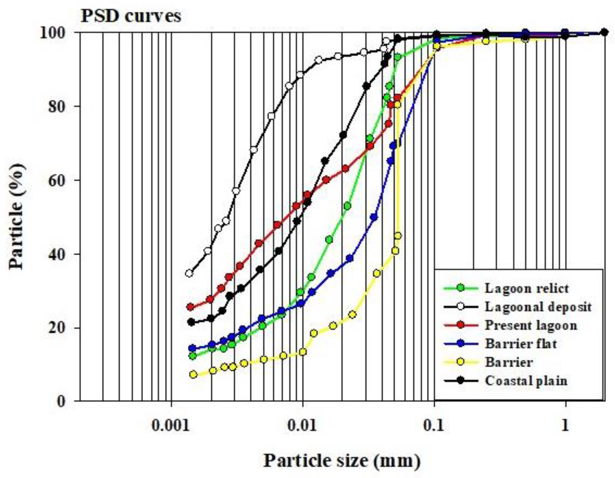
3.2. Particle Size Distribution (PSD) Analysis

PSD analysis and associated granulometric curves, were used to identify specific coastal landforms by emphasizing sedimentary conditions. There are three classes of granulometric curves [14] and each one illustrates a unique sedimentary depositional environment: (1) a “Logarithmic curve” is characteristic of a torrential flow or splay deposit; (2) a “Sigmoid curve” is characteristic of free sediment accumulation; and (3) a “Parabolic curve” is characteristic of an accumulation forced by an obstacle obstructing the flow. Considering the granulometric classes and the shape of the obtained granulometric graphs, the reconstruction of past sedimentary conditions and environments that cannot be detected with the help of remotely sensed documents has been approached. The particle size distribution (PSD) of sediments is one of the principal indicators for understanding the fate of sediments under different conditions [31]. Using particle size distribution data and the resulting graphs, the presence of lagoons, barriers, barrier flats, coastal plains, lagoonal deposits, and lagoon relicts in the study area have been detected (Figure 3). As Figure 3 shows, the particle size distribution curves for the study area display the landform granulometric forms.

Figure 2 shows the six landform types identified in this study and Figure 4 shows the past progradation of seawater and lagoon formation; sediment redeposition during the Holocene and the reworking of loess deposits are drivers of sediment sources. These results are in agreement with those of Kakroodi et al. [15,16] who studied rapid sea-level changes along the Iranian Caspian coast and Ghassemi and Gerzanti (2019) who examined Caspian sediments and loess related to the Gorgan Plain of Turkmenistan. The majority of the volume of the loess in the present study area was deposited in the Pleistocene era [17]; Frechen et al. (2009) discovered that northern Iran’s loess deposits near the Turkmenistan border are composed of a large fraction (more than 80%) of various silt sizes and materials and smaller fractions of various sand sizes and clay particles [32]. The results obtained by Frechen et al. [32] corresponded well with the present study’s PSD analysis, which shows the high amounts of silt at different depths. In the studies conducted by Kakroodi et al. [15], it is observed that, from 1992 to 2012, there were fluctuations in the pro/retrogradation of seawater. Therefore, there has been a backward-facing trend in recent decades. In 2015, Kakroodi et al. reconstructed Late Pleistocene to Holocene Caspian Sea levels in their study using a multi-disciplinary approach and a 27.7 m long core from the southeastern corner of the Iranian Caspian Sea coast in the Gomishan Lagoon [16].

Based on losses from the study area, the results reported by researchers about their origin, and the geopedologic approach conducted [14], the landforms identified in this study can be detected through PSD analysis. Fluxes in energy and seawater fluctuations have affected depositional patterns, and the granulometric curve patterns and conditions of depositions can be tracked through PSD analysis of soil using geomorphic features as a confidence fingerprint. Overall, PSD analysis offers beneficial information about the history of sedimentary conditions, which can help in the reconstruction of past environments [14,15,16].

3.3. Soil Quality Index Models (IQI and NQI)

Soil quality evaluation using IQI and NQI models delineated different quality classes for the discriminated coastal landforms, and highlighted the effect of seawater fluctuations (pro/retrogradations) on land quality. On the other hand, calculating the soil quality indexes and delineating the morphogenic environments and landforms can clarify the effect and relationship of geopedology on LD/development. Salinization is one of the most important issues in coastal areas related to soil and LD. It occurs due to the movement and release of water-soluble salts in an area with little or no concentration of salts. It causes the accumulation of carbonates, sulfates, chlorides, sodium, calcium, and magnesium in surface soil. Salinization can also happen in sediments and pores of rocks, and there are two types: primary and secondary salinization [33]. Primary salinity develops due to the presence of geological materials such as salt rocks, the climate (low rainfall and high evapotranspiration), or due to topography (low altitude areas, closed depressions, areas close to the sea, and areas affected by seawater fluctuations, which also affects the groundwater aquifer).

In contrast, secondary salinity is mainly due to mismanagement and human activity. Salt-affected soils are formed by the influence of ions in the liquid or solid phase, which changes the soil’s physical, chemical, and biological properties [14]. Salinity affects the physicochemical and biological properties of soil, like SOM, E.C., pH, SAR, cations, and anions; therefore, changes in these properties can be used as indicators of LD. Specifically, soilscapes information (for example, the landscape’s pedology) and characteristics, and the composition of soilscapes in landscapes, have been discussed to better understand the relationship between the causes, processes, and the best set of indicators (TDS or MDS sets) for mapping and monitoring LD [14].

The effects of landforms affected by seawater fluctuation and circumstances on LD and development have been investigated based on the fact that the influence of ions in soil can alter soil’s physicochemical and biological properties. On the other hand, a geopedologic approach considers both topography of soils and climate changes. As the study area has been affected by seawater fluctuation [15], these periodic and continual seawater pro/retrogradations laid sediments which brought about the formation and evolution of the landforms. Figure 5 shows that the identified land quality classes are indicated in the 0–20 cm depth maps extracted by the IQI and NQI models run using the TDS and MDS methods. It has been proved that, by considering the IQI and NQI models, soils that were exposed to the seawater have different amounts of ions and variable quantities of physicochemical and biological indicators; in other words, it has been clarified that, by considering all of the factors in determining soil quality, some indicators could affect the assessments. As some indicators that are categorized in the “More is better” branch, for example, SOM and K, in marine environments, these can incorrectly influence the assessment.

An inland water body, known as a coastal lagoon, can be found across all continents, usually oriented parallel to the coast or shoreline and separated from the sea by a barrier. A coastal lagoon is connected to the sea by one or more inlets which can be restricted or may remain open, at least periodically. A lagoon’s shallow water depths seldom can exceed a few meters [34]. Based on the definition of coastal lagoons, these landscapes have special situations in the first few years after exposure to seawater due to the limited ranges of soil quality indicators and because of the limited leaching situations and exceptionally high evapotranspiration in arid and semiarid regions, which can be classified into the lowest quality classes. Due to the limitations of high levels of salinity and ions in these areas, any cultivation is impossible, and they are ranked as the most inferior quality class (class IV). However, in lands far from the coastline that have not been affected by seawater fluctuations for a long time, such as the lands in the southern and southwestern parts of the study area, which, over time, have been affected by rainfall, artificial drainage, and plowing and farming activities, soil quality is currently being improved. The maps obtained with both IQI models, using the TDS and MDS methods, show the enhancement in the quality of these lands, as can be seen in Figure 5. Figure 2 shows the natural remediation in the lagoon deposit and coastal plain areas (Figure 2).

According to the results in Table 3 and Table 4, it is clear that the main effects on indicators of soil and land quality are due to the effect of water-soluble salts, and the presence of water-soluble salts plays a tremendous role in the processes of LD and development.

As shown in Figure 5, for maps derived using the IQI and NQI models ran with TDS and MDS methods, without landform separation, only two identified classes (III and IV) of land quality are identified and the coarseness of the maps limits their usefulness.

3.4. Features Weighting

Values for the contribution of each property (communality), resulting from the factor analysis (F.A.) using a TDS and MDS approach, are presented in Table 3 and Table 4. The effectiveness of each feature in the models depends on the weight assigned to that feature; higher weight characteristics in the TDS or MDS model correspond to a more significant effect on the model, and less impact is assigned to the lower weight characteristics [35]. The weight calculation results in TDS and the MDS models with parameters having the highest weights/effects.

The standard scoring functions suggested by Qi et al. [25] have been used to determine the soil properties (see

Table 5. Scoring functions and its parameters for soil quality variables.

Indicator	Function Type	Lower Limit	Upper Limit	Unit	SSF Equation
SOM	More is better	15	30	%	$M_{\left(x\right)}=\left\{0.9\frac{X-L}{U-L}+0.1,\begin{array}{c}0.1, X<L\\ \\ L\le X\le U\\ \\ 1, X>L\end{array}\right.$
SP	More is better	10	25	%
Fe2+ (DTPA)	More is better	2	32	mg·kg−1
Mn2+ (DTPA)	More is better	10	20	mg·kg−1
Cu2+ (DTPA)	More is better	2	4	mg·kg−1
Zn2+ (DTPA)	More is better	1.5	3	mg·kg−1
K+	More is better	1	5.1	meq·L−1
Sand	Optimal	40	60	%	$O_{\left(x\right)}=\left\{1,\begin{array}{c}0.1, X<L\\ \\ L\le X\le U\\ \\ 0.1, X>L\end{array}\right.$
Silt	Optimal	10	20	%
Clay	Optimal	10	20	%
CaCO3	Less is better	3	55	%
Na+	Less is better	25	250	meq·L−1	$L_{\left(x\right)}=\left\{1-0.9\frac{X-L}{U-L},\begin{array}{c}1, X<L\\ \\ L\le X\le U\\ \\ 0.1, X>L\end{array}\right.$
Ca2+	Less is better	10	30	meq·L−1
Mg2+	Less is better	8	35	meq·L−1
Cl−	Less is better	25	250	meq·L−1
CO32−	Less is better	2	5	meq·L−1
HCO3−	Less is better	5	15	meq·L−1
SO42−	Less is better	10	30	meq·L−1
SAR	Less is better	4	13
EC	Less is better	0.2	2	dS·m−1
pH	Less is better	7.05	8.5

). The upper and lower limits of soil quality rating for IQI and NQI models in TDS and MDS were identified and classified into three categories: More is better, Less is better, and Optimal, see Table 5. Linear functions were used to score data from researchers in different areas [30].

3.5. Soil Quality Rating

Soil quality evaluation is essential for understanding its potential for land use planning, agricultural activities, and the overall health of the environment [30,33,36]. According to the classifications (soil quality grades) in

Table 6. Soil quality rating in IQI and NQI models in TDS and MDS [20].

Soil Quality Index Model	Indicator Method	Soil Quality Grade
		Ι	ΙΙ	ΙΙΙ	ΙV
IQI	TDS	0.76 ≤ IQITDS	0.66 ≤ IQITDS < 0.76	0.56 ≤ IQITDS < 0.66	IQITDS < 0.56
	MDS	0.78 ≤ IQIMDS	0.68 ≤ IQIMDS < 0.78	0.58 ≤ IQIMDS < 0.68	IQIMDS < 0.58
NQI	TDS	0.55 ≤ NQITDS	0.45 ≤ NQITDS < 0.55	0.35 ≤ NQITDS < 0.45	NQITDS < 0.35
	MDS	0.80 ≤ NQIMDS	0.70 ≤ NQIMDS < 0.80	0.60 ≤ NQIMDS < 0.70	NQIMDS < 0.60

, the results indicate that the study area is classified into classes II, III, and IV using each evaluation method and model. In fact, no noticeable differences in the evaluation and classification of the study area have been observed, either as separate landforms or as an integrated study without landform separation using the Nemoro method in both TDS and MDS. However, using the IQI method, it was found that an investigation into the landforms in the study area affected the final maps with the addition of one more class, both for the TDS and MDS, in contrary to evaluating with no segregation. On the other hand, with the separation of landforms, it has been found that the accuracy of classification increased compared to the study method used for the region (no landforms segregation). In the study without landform segregation, the study area was classified into only two classes, III and IV, while using landforms segregation increased classification and added Class II land quality. This method eventually isolated three quality classes: II, III, and IV, for the study area (Figure 5).

Of the 21 study soil parameters examined in the TDS model, SOM, CaCO₃, SP, E.C., pH, Silt, Clay, Na⁺, Ca²⁺, Cl⁻, HCO₃⁻, SAR, Mn²⁺, and Cu²⁺ had the highest repetition in the selection of the MDS model. Low organic matter content is one of the most important limitations of soils in arid and semiarid regions and low soil organic matter reduces fertility and quality, such as nutrient cycle, plant root growth, gas flow intensity, aggregate stability, microorganism activity, etc. SOM is decisive in soil quality stability, crop production, and environmental quality [26]. The predominant mineral carbonate in soils in arid and semiarid regions is calcium carbonate. Surface horizons with less calcium carbonate can be removed by erosion thus exposing the lower horizons with more calcium carbonate. In the study area, most of the soil had calcium carbonate accumulation. The high level of lime and low leaching in arid and semiarid regions increased the pH. High pH (7.10–8.75) is the main factor limiting the absorption of micronutrients, which negatively affects soil quality [3]. Table 3 and Table 4 showed the relationship between pH and sodium and calcium based on the high impact of SAR in determining land quality indices in arid and semiarid regions. The results showed that sodium and calcium affected the selecting SAR directly. On the other hand, physical factors (e.g., S.P.) which were classified as “more is better” have direct relationships with the percentages of silt and clay that have been classified in the optimal category. Since the soils from the study area showed high EC values, and according to the results obtained in present study, severe impacts of sodium and chlorine on EC values are reported. The PC1 column in Table 2, and lagoon relict, lagoon deposit, barrier flat, and coastal plain in Table 3 and Table 4, showed that the items which included EC, Na⁺, and Cl⁻ were frequently selected in the MDS model; through statistical analysis, such a conclusion can be derived to categorized both Na⁺, and Cl⁻ as “less is better” category, like EC [25,28]. The high salinity of the investigated soils, and their effect on the degradation of soil/land quality classes, is mainly due to the high levels of sodium chloride in these soils and which originated from the high concentration of sodium chloride in Caspian Sea water. These results are also strong evidence of the marine nature and the high impact of sea water fluctuations in the region. Also, in this study, heavy metal elements such as iron, manganese, copper, and zinc were studied, and it was found that the effect of copper and manganese on determining the land quality indicators is higher than the other two elements. These results also confirm the marine origin of the landforms in the study area. In a study conducted [37] in Tunisia, scientists studied the effects of the absorption and mobility of the above-mentioned elements in silty clay peloids for medical uses due to the high concentration of them in seawater. It was clarified that, by incorporating a geopedological approach into LD and development studies, results which are much more accurate to the reality of the study area will be created. In addition, the geopedological approach will assess LD and development. According to the results, it has been found that the presence of soluble salts has the highest impact on the degradation and development of coastal lands. For example, lagoon areas with special conditions are the place in which salts accumulate in the soil, and the quality of land in the landforms is reduced. Still, drainage rehabilitation can help reconstitute these areas and land quality classes. On the other hand, agricultural activities, as seen in the study area’s south and southwestern parts, have caused these lands’ revitalization.

3.6. Geopedologic Approach

Incorporating a geopedologic approach helped focus our analysis on both topography and seawater fluctuations derived from climate changes. The unique relationships between SOM, CaCO₃, SAR, SP, E.C., and pH provided a comprehensive approach towards assessing land quality, which could guide precision agriculture and enhance sustainable land management practices.

The study’s classified maps, generated through IQI and NQI models, revealed distinctive land quality classes, with a considerable influence of soluble salts on the assessed criteria. Analysis of the effects of seawater pro/retrogradation on landforms, and the subsequently salinization of these landforms, underscored the importance of geopedologic methods in understanding LD and development in coastal areas [17,18,20].

4. Conclusions

Soil quality assessment using an IQI versus an NQI approach resulted in a much better classification of land quality. The geopedological approach significantly enhanced scientific judgments in land use planning by integrating the disciplines of geomorphology and pedology. Through a detailed analysis of the relationships between landforms and soils, this approach provided a more nuanced understanding of how geologic and geomorphic factors affect soil degradation, soil development, and soil distribution. In the study area, the geopedologic approach identified specific landforms and evaluated their physiochemical properties, contributing to a comprehensive assessment of soil and land quality.

Moreover, the geopedologic approach applied in this study resulted in a clear land quality classification. Targeted soil properties such as electrical conductivity, organic matter, calcium carbonate, sodium absorption ratio, etc., afforded a more holistic perspective on the intricate factors influencing land quality. This approach will support land use planning, particularly in regions affected by unique environmental factors, such as seawater fluctuation in arid and semiarid areas.

Lastly, by considering the region without the segregation of landforms, high-impact elements selected as an MDS may not be accurate enough for the whole region. But when several different landforms are distinguished in the region, the effect of each factor can be clearly discerned. The success of this approach in enhancing land quality assessment and contributing to sustainable land management is relevant in similar systems elsewhere.

In conclusion, the present study highlights the effectiveness of the geopedologic approach, specifically in assessment of soil quality using the IQI model compared to the NQI model. This method significantly improved the land quality classification and demonstrated the synergy between geomorphology and pedology in enhancing scientific judgments for land use planning. The detailed analysis of the relationships between landforms and soils provided a nuanced understanding of how geologic and geomorphic factors influence soil degradation and soil development. The geopedologic approach, which applied in this study, resulted in a clear land quality classification by assessing specific soil properties. This comprehensive perspective on soil’s physico-chemical factors supports effective land use planning, particularly in regions with unique environmental characteristics such as seawater fluctuation in arid and semiarid areas. Additionally, the success of geopedologic approach in understanding the impact of different coastal landforms contributes to more accurate and sustainable land management practices, while also demonstrating its relevance to similar systems at both national and international scales. The study’s findings contribute to the existing theoretical framework by showcasing the practical applications of the geopedologic approach in real-world settings. Furthermore, the direction of future studies is emphasized, recognizing the need for ongoing research in this field to enhance our understanding of land quality dynamics and improve sustainable land management practices. This study suggests that future research should investigate the impact of different coastal landforms on soil and land quality by expanding the applicability of the geopedologic approach.

References

1. Jendoubi, D.; Hossain, M.S.; Giger, M.; Tomićević-Dubljević, J.; Ouessar, M.; Liniger, H.; Ifejika Speranza, C. Local livelihoods and land users’ perceptions of land degradation in northwest Tunisia. Environ. Dev. 2020, 33, 100507. [Google Scholar] [CrossRef]
2. UNESCO. Worsening Land Degradation Impacts 3.2 Billion People Worldwide; United Nations Educational, Scientific and Cultural Organization: Paris, France, 2018. [Google Scholar]
3. Wang, C.; Zhu, D.; Jiang, X.; Zhao, H.; Wang, C.; Yu, F.; Yi, Y. Soil Quality Evaluation and Technology Research on Improving Land Capability—A Case Study on Huanghuaihai Plain in Shandong Province. Agric. Sci. Technol. 2014, 15, 1960. [Google Scholar]
4. Sims, N.C.; Englanda, J.R.; Newnham, G.J.; Alexander, S.; Green, C.; Minelli, S.; Held, A. Developing Good Practice Guidance for Estimating Land Degradation in the Context of the United Nations Sustainable Development Goals. Environ. Sci. Policy 2019, 92, 349–355. [Google Scholar] [CrossRef]
5. Abdullah, H.M.; Islam, I.; Miah, M.G.; Ahmed, Z. Quantifying the Spatiotemporal Patterns of Forest Degradation in a Fragmented, Rapidly Urbanizing Landscape: A Case Study of Gazipur, Bangladesh. Remote Sens. Appl. Soc. Environ. 2019, 13, 457–465. [Google Scholar] [CrossRef]
6. Hossain, M.S.; Eigenbrod, F.; Johnson, F.A.; Dearing, J.A. Unravelling the Interrelationships between Ecosystem Services and Human Wellbeing in the Bangladesh Delta. Int. J. Sustain. Dev. World Ecol. 2017, 24, 120–134. [Google Scholar] [CrossRef]
7. Islam, M.R.; Abdullah, H.M.; Ahmed, Z.U.; Islam, I.; Ferdush, J.; Miah, M.G.; Miah, M.M.U. Monitoring the Spatiotemporal Dynamics of Waterlogged Area in Southwestern Bangladesh Using Time Series Landsat Imagery. Remote Sens. Appl. Soc. Environ. 2018, 9, 52–59. [Google Scholar]
8. Jendoubi, D.; Liniger, H.; Ifejika Speranza, C. Impacts of Land Use and Topography on Soil Organic Carbon in a Mediterranean Landscape (North-Western Tunisia). Soils 2019, 5, 239–251. [Google Scholar] [CrossRef]
9. United Nations Development Programme. The Sustainable Development Goals (SDGs). 2015. Available online: http://www.undp.org (accessed on 23 December 2018).
10. Hoover, D.L.; Bestelmeyer, B.; Grimm, N.B.; Huxman, T.E.; Reed, S.C.; Sala, O.; Seastedt, T.R.; Wilmer, H.; Ferrenberg, S.J.B. Traversing the Wasteland: A Framework for Assessing Ecological Threats to Drylands. BioScience 2020, 70, 35–47. [Google Scholar] [CrossRef]
11. Leng, X.; Feng, X.; Fu, B. Driving Forces of Agricultural Expansion and Land Degradation Indicated by Vegetation Continuous Fields (VCF) Data in Drylands from 2000 to 2015. Glob. Ecol. Conserv. 2020, 23, e01087. [Google Scholar] [CrossRef]
12. Krishna, N.I. Statement on Behalf of the Secretariat of the UN Convention to Combat Desertification; UNCCD: New York, NY, USA, 2008. [Google Scholar]
13. Vogt, J.V.; Safriel, U.; von Maltitz, G.; Sokona, Y.; Zougmore, R.; Bastin, G.; Hill, J. Monitoring and Assessment of Land Degradation and Desertification: Towards New Conceptual and Integrated Approaches. Land Degrad. Dev. 2011, 22, 150–165. [Google Scholar] [CrossRef]
14. Zink, J.A. Geopedology, An Integration of Geomorphology and Pedology for Soil and Landscape Studies; ITC: Enschede, The Netherlands, 2013. [Google Scholar]
15. Kakroodi, A.A.; Kroonenberg, S.B.; Hoogendoorn, R.M.; Mohammd Khani, H.; Yamani, M.; Ghassemi, M.R.; Lahijani, H.A.K. Rapid Holocene Sea-Level Changes along the Iranian Caspian Coast. Quat. Int. 2012, 263, 93–103. [Google Scholar] [CrossRef]
16. Kakroodi, A.A.; Leroy, S.A.G.; Kroonenberg, S.B.; Lahijani, H.A.K.; Alimohammadian, H.; Boomer, I.; Goorabi, A. Late Pleistocene and Holocene Sea-Level Change and Coastal Paleoenvironment Evolution along the Iranian Caspian Shore. Mar. Geol. 2015, 361, 111–125. [Google Scholar] [CrossRef]
17. Ghassemi, M.R.; Garzanti, E. Geology and Geomorphology of Turkmenistan: A Review. Geopersia 2019, 9, 125–140. [Google Scholar]
18. Samiei-Fard, R.; Heidari, A.; Konyushkova, M.; Mahmoodi, S. Application of Particle Size Distribution Throughout the Soil Profile as a Criterion for Recognition of Newly Developed Geoforms in the Southeastern Caspian Coast. Catena 2021, 203, 105362. [Google Scholar] [CrossRef]
19. Schoeneberger, P.J.; Wysocki, D.A. Geomorphic Description System, version 5.0; Natural Resources Conservation Service—National Soil Survey Center: Lincoln, NE, USA, 2017. [Google Scholar]
20. Zinck, J.A.; Metternicht, G.; Bocco, G.; Francisco Del Valle, H. Geopedology, An Integration of Geomorphology and Pedology for Soil and Landscape Studies; Springer International Publishing: Cham, Switzerland, 2016. [Google Scholar]
21. Sparks, D.L.; Page, A.L.; Helmke, P.A.; Loeppert, R.H. (Eds.) Methods of Soil Analysis, Part 3: Chemical Methods; John Wiley & Sons: Hoboken, NJ, USA, 2020; Volume 14. [Google Scholar]
22. Nelson, R.E. Carbonate and gypsum. In Methods of Soil Analysis, Part 2: Chemical and Microbiological Properties; John Wiley & Sons: Hoboken, NJ, USA, 1983; Volume 9, pp. 181–197. [Google Scholar]
23. Dane, J.H.; Topp, C.G. (Eds.) Methods of Soil Analysis, Part 4: Physical Methods; John Wiley & Sons: Hoboken, NJ, USA, 2020; Volume 20. [Google Scholar]
24. Walkley, A.; Black, I.A. An examination of the Degtjareff method for determining soil organic matter, and a proposed modification of the chromic acid titration method. Soil Sci. 1934, 37, 29–38. [Google Scholar] [CrossRef]
25. Qi, Y.; Darilek, J.L.; Huang, B.; Zhao, Y.; Sun, W.; Gu, Z. Evaluating Soil Quality Indices in an Agricultural Region of Jiangsu Province, China. Geoderma 2009, 149, 325–334. [Google Scholar] [CrossRef]
26. Bi, C.J.; Chen, Z.L.; Wang, J.; Zhou, D. Quantitative Assessment of Soil Health under Different Planting Patterns and Soil Types. Pedosphere 2013, 23, 194–204. [Google Scholar] [CrossRef]
27. Congreves, K.A.; Hayes, A.; Verhallen, E.A.; Van Eerd, L.L. Long-term Impact of Tillage and Crop Rotation on Soil Health at Four Temperate Agroecosystems. Soil Tillage Res. 2015, 152, 17–28. [Google Scholar] [CrossRef]
28. Rahmanipour, F.; Marzaioli, R.; Bahrami, H.A.; Fereidouni, Z.; Bandarabadi, S.R. Assessment of Soil Quality Indices in Agricultural Lands of Qazvin Province, Iran. Ecol. Indic. 2014, 40, 19–26. [Google Scholar] [CrossRef]
29. Shukla, M.K.; Lal, R.; Ebinger, M. Determining Soil Quality Indicators by Factor Analysis. Soil Tillage Res. 2006, 87, 194–204. [Google Scholar] [CrossRef]
30. Liu, Z.; Zhou, W.; Shen, J.; Li, S.; He, P.; Liang, G. Soil Quality Assessment of Albic Soils with Different Productivities for Eastern China. Soil Tillage Res. 2014, 140, 74–81. [Google Scholar] [CrossRef]
31. Sadeghi, S.H.; Gharemahmudli, S.; Kheirfam, H.; Khaledi Darvishan, A.; Kiani Harchegani, M.; Saeidi, P.; Gholami, L.; Vafakhah, M. Effects of Type, Level, and Time of Sand and Gravel Mining on Particle Size Distributions of Suspended Sediment. Int. Soil Water Conserv. Res. 2018, 6, 184–193. [Google Scholar] [CrossRef]
32. Frechen, M.; Kehl, M.; Rolf, C.; Sarvati, R.; Skowronek, A. Loess Chronology of the Caspian Lowland in Northern Iran. Quat. Int. 2009, 198, 220–233. [Google Scholar] [CrossRef]
33. Zinck, J.A.; Metternicht, G. Soil Salinity and Salinization Hazard. In Remote Sensing of Soil Salinization; Springer: Berlin/Heidelberg, Germany, 2009; pp. 3–18. [Google Scholar]
34. Kjerfve, B. Coastal Lagoons; Elsevier Oceanography Series; Elsevier: Amsterdam, The Netherlands, 1994; Volume 60, Chapter 1; pp. 1–8. [Google Scholar]
35. Sharma, S.K.; Ramesh, A.; Sharma, M.P.; Joshi, O.P.; Govaerts, B.; Steenwerth, K.L.; Karlen, D.L. Microbial Community Structure and Diversity as Indicators for Evaluating Soil Quality. In Biodiversity, Biofuels, Agroforestry and Conservation Agriculture; Springer: Berlin/Heidelberg, Germany, 2010; pp. 317–358. [Google Scholar]
36. Swanepoel, P.A.; Botha, P.R.; du Preez, C.C.; Snyman, H.A. Physical Quality of a Podzolic Soil following 19 Years of Irrigated Minimum-Till Kikuyu-Ryegrass Pasture. Soil Tillage Res. 2013, 133, 10–15. [Google Scholar] [CrossRef]
37. Khalil, N.; Charef, A.; Khiari, N.; Gomez Pérez, C.P.; Andolsi, M.; Hjiri, B. Influence of Thermal and Marine Water and Time of Interaction Processes on the Cu, Zn, Mn, Pb, Cd and Ni Adsorption and Mobility of Silty-Clay Peloid. Appl. Clay Sci. 2018, 162, 403–408. [Google Scholar] [CrossRef]
Figure 1. (a) The setting of the study area and (b) sampling points.
Environments 11 00020 g001
Figure 2. Digital elevation model (DEM) and contour lines.
Environments 11 00020 g002
Figure 3. Particle size distribution (PSD) curves which are proxies of PSD analysis in each detected landform.
Environments 11 00020 g003
Figure 4. Pro/retrogradation of Caspian Sea water since 1975–2020 (Landsat, USGS).
Environments 11 00020 g004
Figure 5. Land quality classified maps of the study area by landform segregation (Separated) and no landforms segregation (Totally).
Environments 11 00020 g005