Comparison of SCS and Green-Ampt Distributed Models for Flood Modelling in a Small Cultivated Catchment in Senegal


Institut de Recherche pour le Développement (IRD), HydroSciences Montpellier, UMR 5569 CNRS-IRD-UM, 34000 Montpellier, France
*
Author to whom correspondence should be addressed.
Geosciences 2018, 8(4), 122; https://doi.org/10.3390/geosciences8040122
Submission received: 29 January 2018
/
Revised: 27 March 2018
/
Accepted: 29 March 2018
/
Published: 4 April 2018
(This article belongs to the Special Issue Hydrological Hazard: Analysis and Prevention)
Abstract
:The vulnerability to floods in Africa has increased over the last decades, together with a modification of land cover as urbanized areas are increasing, agricultural practices are changing, and deforestation is increasing. Rainfall-runoff models that properly represent land use change and hydrologic response should be useful for the development of water management and mitigation plans. Although some studies have applied rainfall-runoff models in West Africa for flood modelling, there is still a need to develop such models, while many data are available and have not still been used for modelling improvement. The Ndiba catchment (16.2 km2), which is located in an agricultural area in south Senegal, is such catchment, where a lot of hydro-climatic data has been collected between 1983 and 1992. Twenty-eight flood events have been extracted and modelled by two event-based rainfall-runoff models that are based on the Soil Conservation Service (SCS) or the Green-Ampt (GA) models for runoff, both coupled with the distributed Lag and Route (LR) for routing. Both models were able to reproduce the flood events after calibration, but they had to account for that the infiltration processes are highly dependent on the tillage of the soils and the growing of the crops during the rainy season, which made the initialization of the event-based models difficult. The most influent parameters for both models (the maximal water storage capacity for SCS, the hydraulic conductivity at saturation for Green-Ampt) were mostly related to the development stage of the vegetation, described by a Normalized Difference Vegetation Index (NDVI) anomaly. The SCS model performed finally better than the Green-Ampt model, because Green-Ampt was very sensitive to the variability of the hydraulic conductivity at saturation. The variability of the parameters of the models highlights the complexity of this kind of cultivated catchment, with highly non stationary conditions. The models could be improved by a better knowledge of the tillage practices, and a better integration of these practices in the parameters predictors.
1. Introduction
The vulnerability to floods in Africa has increased over the last decades, in terms of human fatalities and economic losses [1], while in most of African countries, flood warning and prevision systems are not existent [2]. Consequently, there is a need for a better knowledge of these events and to improve rainfall-runoff models that could be used in the development of prevision systems. However, up to now, only a few studies have applied rainfall-runoff models in West Africa for flood modelling (e.g., [3,4]) or the analysis of the hydrological processes in small catchments less than some tenth or hundreds of squared kilometers [5,6]. In West Africa, flood prediction usually derive from synthetic guidelines [7] or regional studies [8,9,10]. But, such works are now ancient and could be revisited or developed, while many data are available in West Africa and have not still been used for modelling improvement.
The small agricultural area Thysse Kaymor is one of these catchments that have not been the object of modelling studies at the catchment scale, despite that many hydro-climatic data have been collected. Five nested catchments have been monitored during the period 1982–1992, including rainfall, runoff, and water content and hydrodynamic properties of the soils. The role of the agriculture on the runoff was clearly shown by [11], who claimed that the runoff conditions are first high before the tillage, and then reduce along the rainy season due to the growth of the crops. They also found that the Normalized Difference Vegetation Index (NDVI) could be a good predictor of the runoff conditions. However, modelling was only performed at the plot scale [12], and not at the catchment scale.
The aim of this study is to assess the skill of two well-known event-based models—the Soil Conservation Service (SCS) model and the Green-Ampt (GA) model in reproducing the flood processes in a semi-arid agricultural catchment of Senegal. To understand the behavior of a watershed during a specific rainfall episode, event-based models are often preferred over continuous models since they require less input data [13] and they possibly reduce the complexity of the hydrological processes. However, the event-based models need to set the initial condition for each event, and to relate this condition to an external predictor [14,15]. Therefore, an event-based model must not only be assessed from its skill to reproduce the floods, but also from the goodness of the relationship between the initial condition of the model and the external predictor, which is linked with. The latter part is often neglected, whereas it is the most important. This dual calibration of an event-based model is addressed in this paper, focusing on the relationship of the initial condition and external predictor, such as antecedent precipitation, event-rainfall characteristics, or satellite-derived normalized difference vegetation index (NDVI) to represent the vegetation stage.
2. Study Area and Data Collection
This study was conducted using data and catchment description from hydrological campaign reports done between 1983 and 1990 by two institutions (Office de la Recherche Scientifique et Technique Outre-Mer (now IRD) and the Institut Sénégalais de Recherche Agricole) in the Thysse Kaymor area.
2.1. Ndiba Catchment
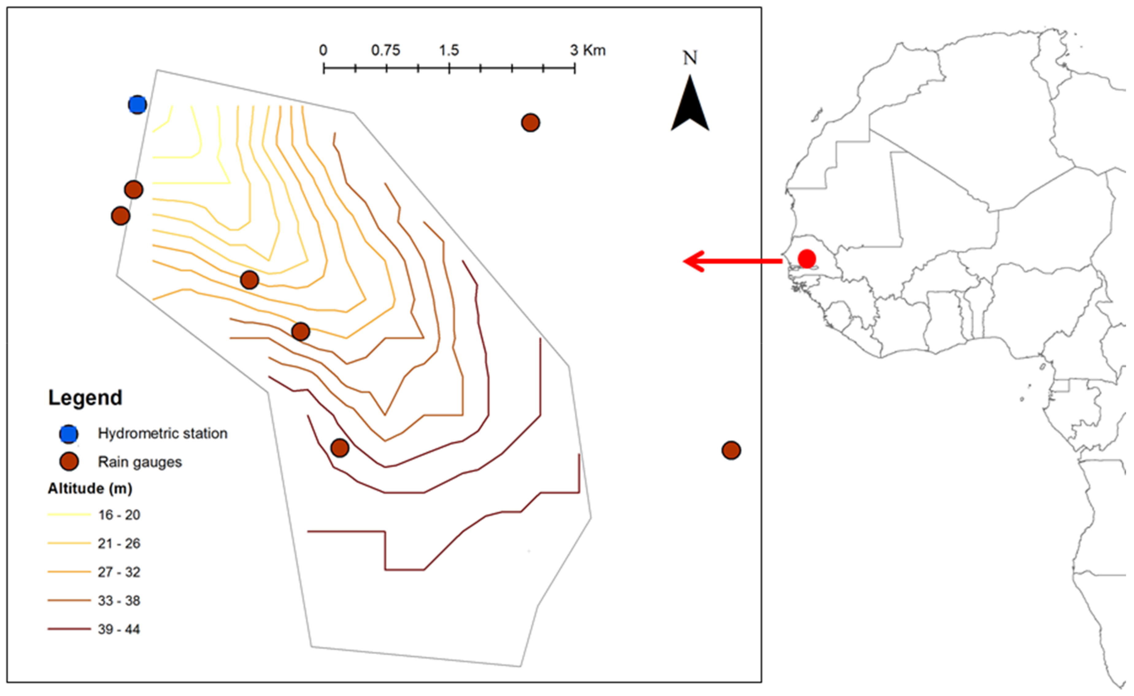
The Ndiba catchment (16.2 km2) is situated in the rural community of Thysse Kaymor, in the Sine Saloum region in southern Senegal (Figure 1). The elevations range between 13 and 45 m, and the slope is about 1%. The Ndiba catchment is mostly (over 50%) cultivated (millet and groundnut), and the other parts are bush areas [16].
The Ndiba catchment, as most of the Thysse Kaymor’s region, is characterized by sandy soils at the surface, but the proportion of clay increases with depth especially between 0.6 and 1.5 m depth [17]. The soil porosity was assumed to decrease with the depth between 0.31 and 0.25 cm3·cm−3 [18]: these values were obtained from experimental measurements of both water content θ and head pressure h at depths 10, 20, 30, 40, 60, 80, 100, 120, 140, 160 cm, in two sites, with either artificial rainfall or Müntz experiment; when the soil saturation was not reached, the water content at saturation was extrapolated from the experimental points (h,θ). The hydraulic conductivities at saturation ranged between 10 and 50 mm·h−1, depending on the type of tillage (perpendicular or parallel to the slope) and the cumulative rainfall since the last tillage [19]; the results were obtained from 48 infiltration tests that were performed by a disk infiltrometer, each test for a different site within an 900 m2 area; the potential storage of water in these areas was estimated to 170 mm in the first 170 cm. During the first rainfall events at the beginning of the wet season, before tillage, the runoff coefficients are usually high since the soils are almost bare due to animal grazing and soil crusting. Then, the runoff coefficient tends to decrease gradually as the amount of vegetation increase during the growing season [11,20].
2.2. Rainfall and Runoff Data
Ndiba rainfalls were continuously registered from seven rain gauges (Precis-Mecanique with tipping buckets, surface 400 cm2, graphical recording with daily rotation) in and around the catchment (Figure 1). The mean rainfall for the catchment during the period 1983–1990 was 612.5 mm, and years 1983 and 1984 were particularly dry, as the annual rainfall was less than 500 mm. These years were characterized by a severe drought that affected West Africa since the 1970’s. The rainy season occurred during summer months, the maximal rainfall generally occurred in August and its mean value is 183 mm.
Gauging information was available at the hydrometric station of Ndiba (altitude = 13 m). The water levels were continuously recorded by a mechanical OTT 10 stream gauge, between 1983 and 1990. Sixty-four gauging have been performed between 1985 and 1988, up to the water level 160 cm, corresponding to a discharge of 58 m3·s−1. Those gauging were correctly located around a unique and reliable rating curve. Rainfall and runoff data for Ndiba catchment were extracted from the SIEREM database (http://www.hydrosciences.fr/sierem/) for the period 1983–1990, with a 5-min time interval. Twenty-eight rainfall-runoff events were selected for the study, and were delimited by periods of 48 h when rain intensity did not exceed 1 mm·h−1; in addition, the events were definitely selected if the maximal rainfall amount was more than 10 mm and the peak flow more than 1 m·s−1. Table 1 shows their main characteristics.
The durations of the events ranged from 0.5 to 14.25 h. The rainfall intensity was generally important at the beginning of the precipitations and decreased along the event. The peak flows ranged from 1.06 to 56.7 m3·s−1 at the outlet of Ndiba catchment. The runoff coefficients ranged from 0.01 to 0.58. Three events had a maximal discharge that was higher than 50 m3·s−1: these events were the first floods occurring at the beginning of the rainy season, and had the highest runoff coefficient (cf. Table 1).
2.3. Initial Soil Moisture Predictor
Event-based models predictions often depend on the initial moisture condition of the catchment [13], which should be assessed by measurements, or, in our case, reliable predictors. The base flow at the beginning of an event can be used as a predictor of initial moisture conditions in humid climates, but not in most of Sahelian small catchments because there is no flow before the floods. Other predictors are commonly used to define soil moisture conditions, such as the Antecedent Precipitation Index (API), which is given by [21]:
where Pj is the rainfall occurring the day j and APIj−1 the index of the previous day. It is multiplied by k, which is a factor that has to be calibrated. The API is computed from daily measurements that were available at the rain gauges.
2.4. Normalized Difference Vegetation Index
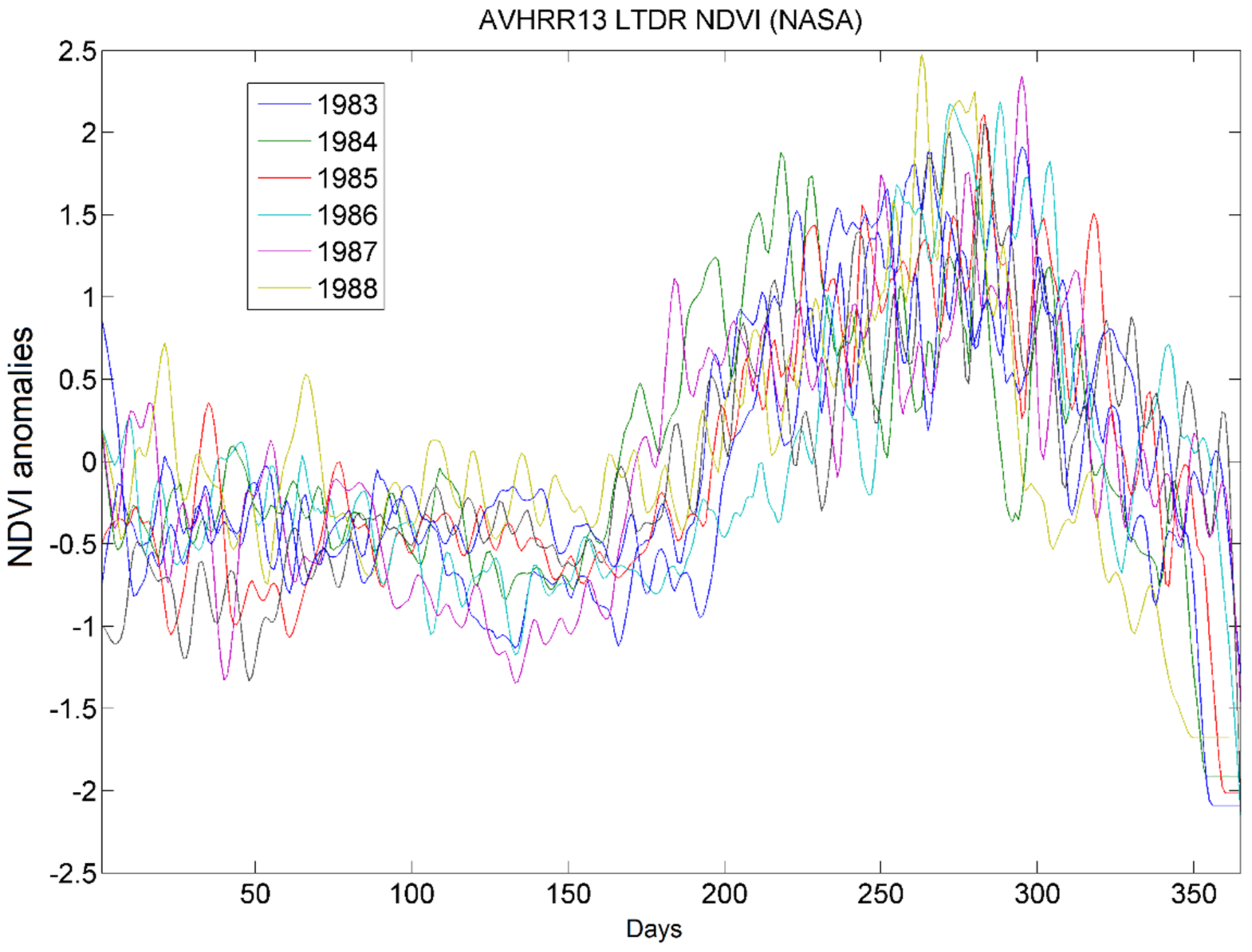
For cultivated catchments, the growth of the vegetation often induces a non-stationarity of the hydrological behavior of the catchment, and consequently, of the model parameters [22,23]. Such variability requires to be related to a reliable descriptor of the growth of the vegetation. The Normalized Differential Vegetation Index (NDVI) was used here as a proxy to monitor the seasonal evolution of vegetation, as shown by [11]. The NDVI daily time series have been retrieved from the NASA’s land long term data record (LTDR) project (available online at: https://ltdr.modaps.eosdis.nasa.gov), which aims to produce a global set of data at a 0.05° spatial resolution, which were collected from AVHRR and MODIS instruments for climate studies [24]. The algorithms used to derive the Normalized Differential Vegetation Index (NDVI) from daily surface reflectance are described in [25,26]. The whole database processing is detailed in [24].
The temporal evolution for the years 1983 to 1988 of NDVI over the Ndiba catchment indicates a very close annual cycle with the maximum vegetation development during the summer (Figure 2).
3. Rainfall-Runoff Modelling
The models were performed within the Atelier Hydrologique Spatialisé (ATHYS) modelling platform, which was developed at the Hydrosciences Montpellier laboratory [27,28]. ATHYS brings together a large set of distributed models within a consistent and easy-to-use environment, including processing of hydrometeorological and geographical data. ATHYS is an open software, which can be downloaded for Windows or Linux (www.athys-soft.org).
The distributed models operated over a grid mesh of regular squared cells. The basic information was brought by a Digital Elevation Model (DEM), which supplied elevation, slope, upstream area, and flowpath for each cell. Here, we used the Advanced Spaceborne Thermal Emission and Reflection Parameter (ASTER) DEM, projected to a UTM horizontal resolution of 30 m. Then, the rainfall was interpolated over the grid cells via the inverse distance interpolation method, at every time step, here 5 min. The runoff models (here, SCS and Green-Ampt) operated thus with 30 m cell size and 5 min time step. Each cell produced a cell-hydrograph at the outlet of the catchment, depending on the runoff model and the routing model (here, the distributed lag and route model). The complete flood hydrograph at the outlet of the catchment was finally obtained as the sum of the cell-hydrographs.
3.1. SCS Runoff Model
The United States Soil Conservation Service developed an empirical model to estimate runoff losses [29]. To date, the SCS method is one of the most popular runoff models, and it was the object of many improvements as well in the formulation of the model as in the interpretation of its parameters (see [30] for a review).
Although it was first designed to relate the cumulated runoff and rainfall at the event scale, it is possible to integrate time into this model to predict infiltration rates [31,32]. The SCS model that is considered here gives the instantaneous runoff at any time of the event [32]:
where Pe(t) is the effective rainfall at time t, Pb(t) the precipitation at time t, P(t) the cumulative rainfall since the beginning of the event. S is the maximal water storage capacity at the beginning of the event. The runoff coefficient is expressed by the quantity that multiplies Pb(t), in the second member of the previous equation; it increases with the cumulative rainfall and tends to 1 when the cumulative rainfall tends to infinity.
To consider that the runoff coefficient decreases during periods when no rain occurs, a linear decrease of the cumulated rainfall was considered through a discharge coefficient ds [T−1] [13,33]:
The parameters of the model are S and ds. The S parameter directly controls the main flood peak and volume, while ds contributes to adjust the different flood peaks and volumes resulting from successive rainfalls within a given event. Note that the ds parameter emulates some kind of variable infiltration rate, which depends on the cumulated rainfall P(t). The S and ds parameters were considered to be constant over the catchment, so that the distribution only concerned the rainfall interpolated for each cell.
3.2. Green-Ampt Model
Green-Ampt model [34] is based on physical measurable parameters and describes a hortonian process of water infiltration. The infiltration capacity f(t) is expressed by the following equation:
where F(t) is the cumulated infiltration [L], θs the saturated soil moisture [L3·L−3], θi the initial soil moisture [L3·L−3], Ks the hydraulic conductivity at saturation [L·T−1] and Ψ the suction [L].
As for the SCS runoff model, the GA parameters were considered to be constant over the catchment, although the land use and the soil types were probably not homogeneous over the catchment. The parameters were thus considered as averaged values over the catchment, in order to be coherent with sparse data about the soil properties.
3.3. Routing Model
SCS and Green-Ampt models were coupled to a lag and route model at the cell scale, to produce a cell-hydrograph at the outlet of the catchment, calculated by:
where A was the cell-area [L2], Pe the effective rainfall [L], Tm the routing time [T]), and Km the lag time [T] from the cell m to the outlet.
This model, available in ATHYS, was already used by [33]. It simply enables the Unit Hydrograph theory, by using the impulse response function:
The routing time Tm was calculated from the length lk and the flux velocity Vk of each k-cell between the m-cell and the outlet of the catchment. The lag time Km was assumed to be linearly dependent of the routing time Tm: Km = K0·Tm. In the following, the velocity Vk was considered as the same for all of the cells: Vk = V0, and K0 as a constant of the catchment.
The routing time Tm and lag time Km induced an actual distribution of the travel times of the runoff over the catchment: the farther from the outlet the cell m is, the larger the routing time and the lag time are. As mentioned above, the complete flood hydrograph at the outlet of the catchment was obtained by the sum of all the cell-hydrographs.
The complete models were denoted after either SCS-LR or SCS, and GA-LR or Green-Ampt.
3.4. Model Calibration
SCS-LR and GA-LR models parameters were either preset from field measurements or empirical/physical consideration, or calibrated using the BLUE (Best Linear Unbiased Estimator) method. In this latter case, the objective consists of minimizing the cost function, J(x) in order to obtain the optimal values of the variables that are stored in a control vector, x [35]:
The control vector x, size n, contains the set of n variables to be optimized, i.e., the model parameters; xb is the background vector of size n, which contains the a priori values of the control vector variables. y° is a vector of size p, which contains the p observations to be considered. H is the observation operator, i.e., the rainfall-runoff model, and supplies the predicted runoff. B (size n × n) and R (size p × p) are the error covariance matrices, respectively, associated to the background, xb, and the observations, yo. The cost function J(x) thus quantifies both the distance between the control vector, x, and the background, xb, and the distance between the runoff predicted by the model and the observed runoff, y°, weighted, respectively, by the error covariance matrices B and R. The smaller the covariance in B is, the closer to the background the control vector is; the smaller the covariance in R is, the closer to the observation the output of the model is.
As a gradient method, the BLUE method allows for a quick computation of the optimized parameters. The parameters were in our case considered as independent (null covariance) and a large variance was considered in the B matrix, in order that the parameters would be low related with the background. This made that the cost function J(x) was actually equivalent to any form of quadratic error between the predicted and observed runoff.
For sake of simplicity, the efficiency of the model was also expressed by the Nash-Sutcliffe coefficient NS:
where Xi and Yi are the observed and simulated discharges for i-time steps, and the mean value of the observed discharges during the event. The closer NS is from 1, the better the correlation between the observed and simulated discharges.
4. Results
4.1. SCS-Model Calibration
4.1.1. Estimation of the SCS-Model Parameters
As said above, the SCS-LR parameters were either preset from field measurements or empirical/methodological consideration, or calibrated by using the BLUE method. The ds parameter was set in order to remove the small floods due to secondary rainfalls, which were not seen in the observed data. A convenient value ds = 8 d−1 was kept as a constant for all of the events. The parameters V0 and K0 were found to be strongly dependent, so the K0 parameter was empirically set as K0 = 0.75 for all of the events.
Then, a simultaneous calibration of S and V0 parameters was realized by using the BLUE method for each event. For the 28 selected events, NS values ranged from 0.30 to 0.99 (median = 0.87), showing for most events a good agreement between observed and calibrated discharges. S parameter values ranged from 15.2 to 175.2 mm (median = 92 mm) and V0 from 0.85 m·s−1 to 5.8 m·s−1 (median = 1.68 m·s−1), Table 2.
No correlation could be found between the velocity V0 and other event feature, such as peak flow and initial water content. The variation of the velocity might be mainly due to uncertainties in time of the recording mechanical gauges. Such uncertainty can reach some tenth of minutes, and due to the short response time of the catchment, can impact the V0 value a lot.
4.1.2. Relation between S and Antecedent Moisture Indicator
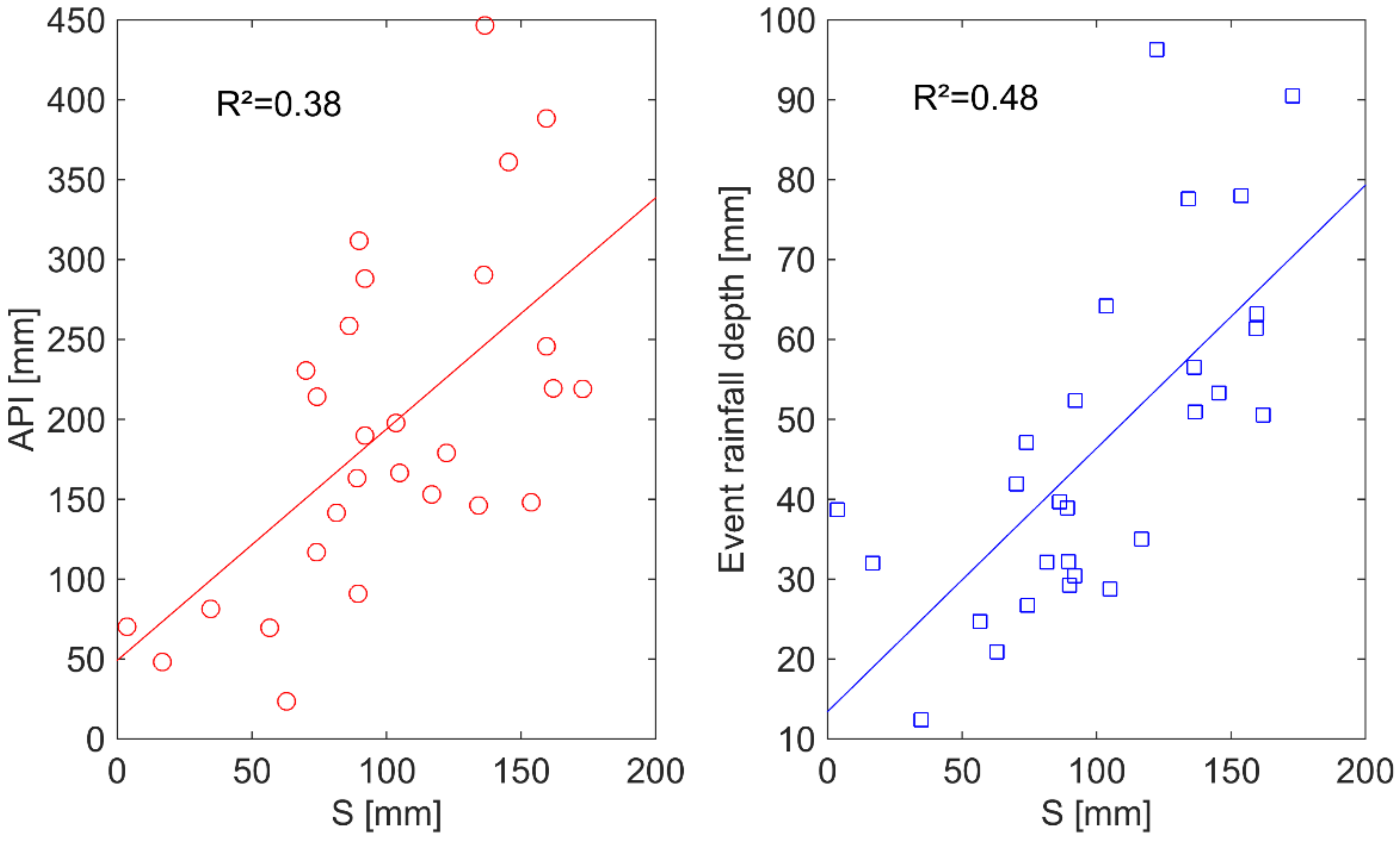
The calibrated values of S for SCS-model for all of the flood events were compared with the previous soil moisture indicator described before (API). For this model, the relation S-API was significant, although weak (R2 = 0.38, PFisher < 1%), but exhibited an opposite correlation to what could be expected (Figure 3). The maximal capacity of retention was indeed supposed to decrease with increased wetness conditions. For example, in a small mountainous Mediterranean catchment, [13] found a negative correlation between S and API, with a Pearson correlation coefficient r = −0.68). But, in the Ndiba catchment, the wetter the soil initially was, the lesser the runoff was. It was probably due because the classical role of the water content before the flood should be here a secondary factor, and that other phenomena would play a major role in the hydrological response of the catchment. It was clear that the tillage of the soil indeed modified a lot the runoff: for example, the highest runoff, consequently, a small S, was obtained for the first floods of the rainy season, consequently, a low API, when no tillage has been made. But, as we had no data about the tillage practices during the rainy season, it was not possible to precisely quantify the role of the tillage on the runoff.
4.1.3. Relation between S and NDVI
As pointed out by [11], the Sahelian agricultural catchments are prone to highly non stationary conditions due to the tillage of the soils and the growth of the plants. The calibrated values of S were then related to the NDVI index, which was associated to the development of the vegetation. A significant, but weak (R2 = 0.29, PFisher < 1%), correlation was found again, which denoted the role of the vegetation in the increase of the maximal water storage capacity of the soil when the plants grow. Note that API and NDVI were dependent, since a linear relationship could be drawn between both indexes, with R2 = 0.47, when considering the values that are corresponding to our 28 events data base. Thus, the positive correlation between the calibrated S values and API would be an artefact due to the development of the vegetation.
4.1.4. Relation between S and Rainfall Depth
The calibrated S parameter of SCS-model was also correlated with the rainfall depth. As shown in Figure 3, S tended to increase with rainfall depth giving almost a linear relation between S and rainfall depth (R2 = 0.48, PFisher < 1%). The relation between rainfall depth and the S parameter was not expected whilst using the SCS-model; but, some studies (among other [36,37]) showed a relation between the CN curve number (consequently S) and the rainfall depth, for high infiltration sandy soils: CN decreases (consequently S increases) with rainfall depth. A possible explanation was given by [38], who claimed that higher rainfall depths increase the flooded part of the soil, and that water rises up to the plants bottom and infiltrates more than in the crusted soil.
4.2. Green-Ampt Model Calibration
An alternative model set-up was considered, with the Green-Ampt model for infiltration. As for the SCS model, the Green-Ampt parameters were either preset or calibrated by the BLUE method. A mean constant value of the soil moisture at saturation state was applied, θs = 0.30 cm3 cm−3, according the field measurements [18]. The initial soil moisture value at the beginning of an event was considered empirically as a linear function of the API index: θi = API/2000; the initial water content thus ranged between 0.02 and 0.22 cm3·cm−3. A suction value of 75 mm was applied, which corresponds to a mean value found in literature for the sandy loam soils [39]. The K0 parameter was set as K0 = 0.75, the same value than for SCS-LR.
Then, simultaneous calibration of hydraulic conductivity Ks and velocity V0 was performed by using the BLUE method. The median NS coefficient was 0.88. The median calibrated Ks value was 31.8 mm·h−1, which looked in agreement with the values measured in the catchment [19]. However, the calibrated Ks values varied widely between 1 and more than 60 mm·h−1 at the event scale. The median calibrated V0 was 1.34 m·s−1.
4.3. Seasonal Evolution of the Ks Parameter Linked with NDVI Anomalies
The calibrated values of the Ks parameter were correlated with the NDVI anomalies (R2 = 0.44, PFisher < 1%, Figure 4). This result indicates that the variation that was observed through the year in hydraulic conductivity was partly driven by the evolution of vegetation growth during the rainy season, as pointed out by [11]. This hydrologic behaviour can thus be reproduced by the Green Ampt model with varying infiltration rates during the wet season, according to the NDVI anomalies. Note that the Green-Ampt model scored better than the SCS model, when considering the relationship with NDVI and the main variable parameter of each model: S for SCS and Ks for Green-Ampt.
4.4. Predictive Scores of the Models
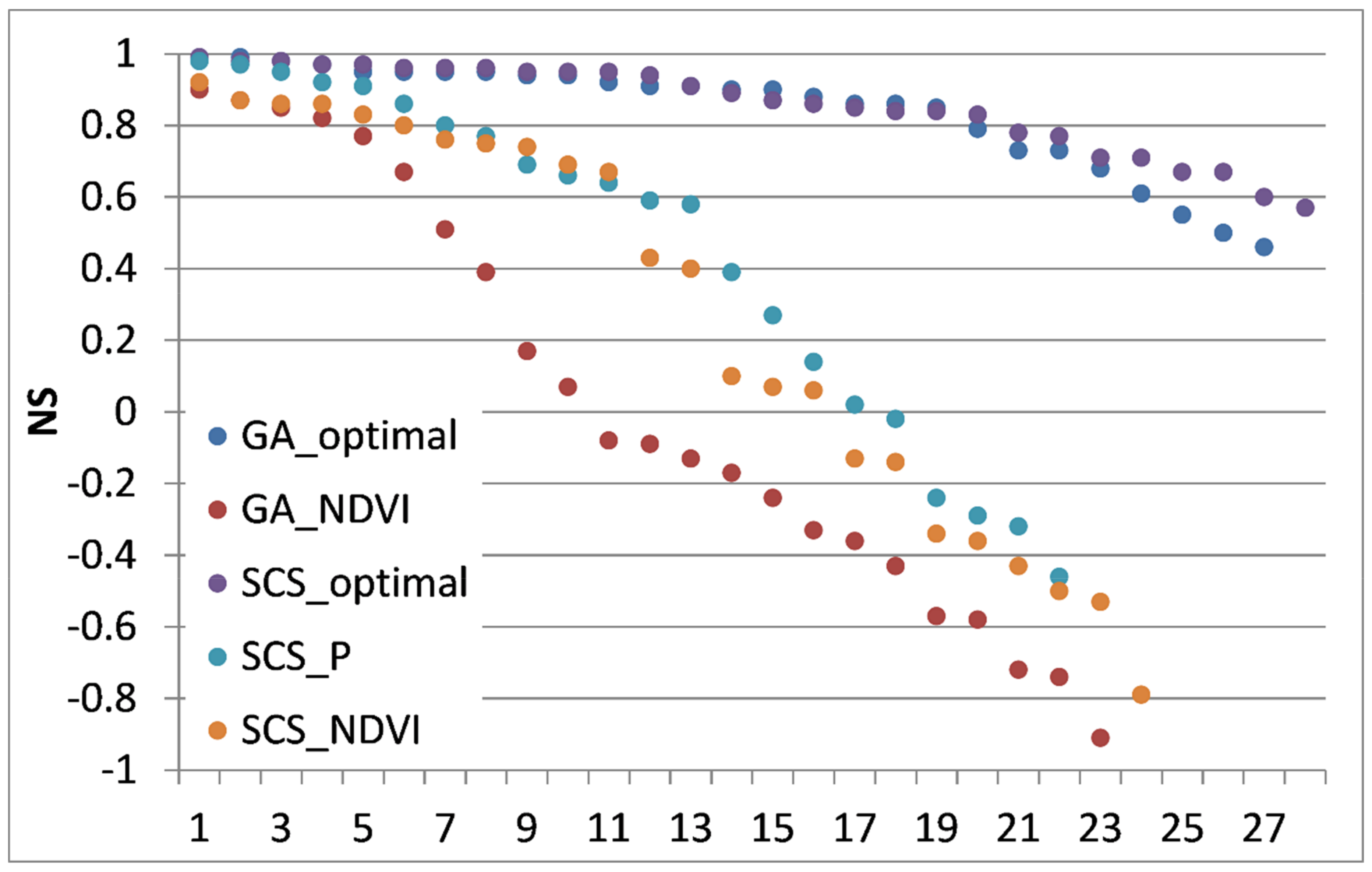
The actual goodness of the models was expressed by the predictive scores, i.e., the NS values that were obtained with the predicted values of S (for SCS) or Ks (for Green-Ampt). The NS values of the 28 events were sorted by descendant order for each model, using the different relationships that were considered as significant (Figure 5): S-NDVI and S-P for SCS, Ks-NDVI for GA. The best predictive scores were achieved for SCS when using the S-P relationship (median NS = 0.33), whereas Green-Ampt when using the Ks-NDVI relationship offered the worst predictive score (media NS = −0.21); SCS scored better when using NDVI (median NS = 0.08), although the R2 was higher for Ks-NDVI than for S-NDVI. This result is due to the fact that GA is very sensitive to Ks, whereas the sensitivity of SCS with S is less. So, SCS globally scored better than Green-Ampt, in terms of predictive scores. However, using a predictor of S, like the rainfall amount, is not appropriate for applications, such as flood forecasting, because the rainfall amount is not known at the moment of the forecast. In this case, it would be preferable to use SCS with the NDVI predictor for S.
The predictive scores of the model, however, remained rather low. It could be because the calibrations of the models were not optimal: maybe it would be worth to consider that some other parameters had to vary from an event to another (e.g., ds or Ψ); or, because the models were not enough appropriate for this kind of catchment; but we think that the low predictive scores were mostly due because we had not information about the dates and the kind of tillage. Ndiaye et al. [19] showed indeed that tillage had a significant effect on runoff, depending on the type (along or across the slope), and that the effect of the tillage disappeared after nearly 170 mm of cumulated rainfall since the date of tillage. Although vegetation growth should be clearly conditioned by tillage, the NDVI index was probably not efficient enough to restore accurately the tillage practices during the rainy season. We suggest first searching in this direction for improving the models.
5. Conclusions
The goal of this study was to evaluate the efficiency of event-based rainfall-runoff model, such as SCS-LR or GA-LR for flood prediction in a small catchment that is located in south Senegal. Twenty-eight flood events were chosen to compare the efficiency of both event-based models.
The application of the SCS-model was found satisfactory to reproduce the observed discharges after calibration of its parameters. However, the initial condition of the model could not be predicted as usual, in relation with the water content of the soil at the beginning of the event. The API index, derived from the antecedent rainfalls, was positively correlated with the S parameter, whereas the SCS model usually considers that the correlation should be negative. The S values were also correlated to the NDVI during the event. That is in agreement with the role of the growth of the plants, which induces highly non-stationary conditions for the hydrological response of the catchment, as noted by various authors, and the initial soil moisture conditions should be a secondary factor. The S values were also related to the cumulated rainfall of the event, which finally appeared as the best predictor for S.
The Green-Ampt model results indicated its adequacy to reproduce the flood events in the catchment. As for the SCS-CN model, the correlation of the model parameters with antecedent precipitation was positive, whereas it was expected to be negative. However, a significant correlation between the hydraulic conductivities (Ks) for each event and the normalized difference vegetation index was observed, highlighting the influence of vegetation cover on soil infiltration properties. The Green-Ampt parameters were in agreement with the measured, e.g., hydraulic conductivity at saturation, or estimated values. But, Green-Ampt finally scored less than SCS, because a high sensitivity to the Ks parameter.
At this point, however, the predictive scores of the models are still low when considering the NS values that were obtained with the best predicted values of S or Ks. The main reason seems to be that the tillage practices are not actually taken into account in the models, nor in the predictors (e.g., NDVI) of the parameters of the models. This seems to be the main point to study for the improvement of the predictive scores of the models. In addition, added value could be brought by considering the whole nested set of catchments in Thysse Kaymor.
To conclude, it is worth noting the interest of such existing large data sets dating from the 80’s, even before, Thysse Kaymor being an example among other. As these data are still underemployed for modeling benchmark and hydrological processes understanding, they could fill a gap concerning flood predicting in West Africa (e.g., T-years return period flood), and bring more confidence in designing small hydraulic works in small (ponding areas, culverts) as well as large (dams, bridges) catchments.
Acknowledgments
We thank the editors M. Piña and M. Li, and three anonymous reviewers for their valuable help in improving the quality of the paper. We are also very grateful to Nathalie Rouché and Jean-Emmanuel Paturel for providing the rainfall-runoff data used in this study.
Author Contributions
Christophe Bouvier and Yves Tramblay conceived and designed the modelling protocol and contributed to the materials; Christophe Bouvier, Lamia Bouchenaki and Yves Tramblay analyzed the data; Christophe Bouvier and Lamia Bouchenaki wrote the paper.
Conflicts of Interest
The authors declare no conflict of interest.
References
- Di Baldassarre, G.; Montanari, A.; Lins, H.F.; Koutsoyiannis, D.; Brandimarte, L.; Blöschl, G. Flood fatalities in Africa: From diagnosis to mitigation. Geophys. Res. Lett. 2010, 37, L22402. [Google Scholar] [CrossRef]
- Tschakert, P.; Sagoe, R.; Ofori-Darko, G.; Codjoe, S.N. Floods in the Sahel: An analysis of anomalies, memory, and anticipatory learning. Clim. Chang. 2010, 103, 471–502. [Google Scholar] [CrossRef]
- Amoussou, E.; Tramblay, Y.; Totin, H.; Mahé, G.; Camberlin, P. Dynamics and modelling of floods in the river basin of Mono in Nangbeto, Togo/Benin. Hydrol. Sci. J. 2014, 59, 2060–2071. [Google Scholar] [CrossRef]
- Komi, K.; Neal, J.; Trigg, M.A.; Diekkrüger, B. Modelling of flood hazard extent in data sparse areas: A case study of the Oti River basin, West Africa. J. Hydrol. Reg. Stud. 2017, 10, 122–132. [Google Scholar] [CrossRef]
- Cappelaere, B.; Vieux, B.E.; Peugeot, C.; Maia, A.; Séguis, L. Hydrologic process simulation of a semiarid, endoreic catchment in Sahelian West Niger: 2. Model calibration and uncertainty characterization. J. Hydrol. 2003, 279, 244–261. [Google Scholar] [CrossRef]
- Le Lay, M.; Saulnier, G.M.; Galle, S.; Séguis, L.; Metadier, M.; Peugeot, C. Model representation of the Sudanian hydrological processes: Application on the Donga catchment (Benin). J. Hydrol. 2008, 363, 32–41. [Google Scholar] [CrossRef]
- FAO. Crues et Apports. Manuel Pour L’estimation des Crues Décennales et des Apports Annuels Pour les Petits Bassins Versants non Jaugés de L’afrique Sahélienne et Tropicale Sèche; Bulletin FAO D’irrigation et de Drainage: Rome, Italy, 1996; Volume 54, p. 265. ISBN 92-5-203874-4. (In French) [Google Scholar]
- Albergel, J.; Chevalier, P.; Lortic, B. D’Oursi à Gagara: Transposition d’un modèle de ruissellement dans le Sahel (Burkina-Faso). Hydrol. Cont. 1987, 2, 77–86. (In French) [Google Scholar]
- Bouvier, C.; Desbordes, M. Un modèle de ruissellement pour les villes de l’Afrique de l’Ouest. Hydrol. Cont. 1990, 5, 77–86. (In French) [Google Scholar]
- Lamachere, J.M.; Puech, C. Cartographie des états de surface par télédétection et prédétermination des crues des petits bassins versants en zones sahélienne et tropicale sèche. In L’hydrologie Tropicale: Géoscience et Outil Pour le Développement; International Association of Hydrological Sciences: Wallingford, UK, 1996; p. 238. (In French) [Google Scholar]
- Séguis, L.; Bader, J.C. Modélisation du ruissellement en relation avec l’évolution saisonnière de la végétation (mil, arachide, jachère) au centre Sénégal. Revue Sci. L’eau 1997, 4, 419–438. (In French) [Google Scholar] [CrossRef]
- Bader, J.C. Modèle analogique de ruissellement à stockage de surface: Test sur parcelles et extrapolation sur versant homogène. Hydrol. Sci. J. 1994, 39, 569–592. (In French) [Google Scholar] [CrossRef]
- Tramblay, Y.; Bouvier, C.; Martin, C.; Didon-Lescot, J.F.; Todorovik, D.; Domergue, J.M. Assessment of initial soil moisture conditions for event-based rainfall–runoff modelling. J. Hydrol. 2010, 387, 176–187. [Google Scholar] [CrossRef]
- Berthet, L.; Andreassian, V.; Perrin, C.; Javelle, P. How crucial is it to account for the antecedent moisture conditions in flood forecasting? Comparison of event-based and continuous approaches on 178 catchments. Hydrol. Earth Syst. Sci. 2009, 13, 819–831. [Google Scholar] [CrossRef]
- Tramblay, Y.; Amoussou, E.; Dorigo, W.; Mahé, G. Flood risk under future climate in data sparse regions: Linking extreme value models and flood generating processes. J. Hydrol. 2014, 519, 549–558. [Google Scholar] [CrossRef]
- Valentin, C. Les Etats de Surface des Bassins Versants de Thysse Kaymor (Sénégal); Rapport ORSTOM 35.489; Office de la Recherche Scientifique Et Technique Outre-Mer (ORSTOM): Dakar, Senegal, 1990. (In French) [Google Scholar]
- Diome, F. Rôle de la Structure du sol Dans son Fonctionnement Hydrique. Sa Quantification par la Courbe de Retrait. Ph.D. Thesis, Université Cheikh Anta Diop, Dakar, Senegal, 1996; p. 131. (In French). [Google Scholar]
- Albergel, J.; Bernard, A.; Ruelle, P.; Touma, J. Hydrodynamique des Sols. Bassins Expérimentaux de Thysse Kaymor. Rapport de la Campagne de Mesures Fev–Avr 1988. 1989. Available online: http://horizon.documentation.ird.fr/exl-doc/pleins_textes/doc34-05/27469.pdf (accessed on 30 March 2018).
- Ndiaye, B.; Esteves, M.; Vandervaere, J.P.; Lapetite, J.M.; Vauclin, M. Effect of rainfall and tillage direction on the evolution of surface crusts, soil hydraulic properties and runoff generation for a sandy loam soil. J. Hydrol. 2005, 307, 294–311. [Google Scholar] [CrossRef]
- Rodier, J.A. Caractéristiques des Crues des Petits Bassins Versants Représentatifs au Sahel; Cahiers ORSTOM, Série Hydrologie; Office De La Recherche Scientifique Et Technique Outre-Mer (ORSTOM): Dakar, Senegal, 1985; Volume XXI, pp. 3–26. (In French) [Google Scholar]
- Kohler, M.A.; Linsley, R.K. Predicting Runoff from Storm Rainfall; Res. Paper 34; U.S. Weather Bureau: Washington, DC, USA, 1951.
- Zhang, L.; Wang, J.; Bai, Z.; Lv, C. Effects of vegetation on runoff and soil erosion on reclaimed land in an opencast coal-mine dump in a loess area. Catena 2015, 128, 44–53. [Google Scholar] [CrossRef]
- Hunink, J.E.; Eekhout, J.P.C.; de Vente, J.; Contreras, S.; Droogers, P.; Baille, A. Hydrological Modelling Using Satellite-Based Crop Coefficients: A Comparison of Methods at the Basin Scale. Remote Sens. 2017, 9, 174. [Google Scholar] [CrossRef]
- Pedelty, J.; Devadiga, S.; Masuoka, E.; Brown, M.; Pinzon, J.; Tucker, C.; Vermote, E.; Prince, S.; Nagol, J.; Justice, C.; et al. Generating a Long-term Land Data Record from the AVHRR and MODIS Instruments. In Proceedings of the IEEE International Geoscience and Remote Sensing Symposium (IGARSS 2007), Barcelona, Spain, 23–28 July 2007; Institute of Electrical and Electronics Engineers: New York, NY, USA, 2007; pp. 1021–1025. [Google Scholar]
- Vermote, E.F.; Kaufman, Y.J. Absolute calibration of AVHRR visible and near-infrared channels using ocean and cloud views. Int. J. Remote Sens. 1995, 16, 2317–2340. [Google Scholar] [CrossRef]
- Saleous, N.Z.; Vermote, E.F.; Justice, C.O.; Townshend, J.R.G.; Tucket, C.J.; Goward, S.N. Improvements in the global biospheric record from the Advanced Very High Resolution Radiometer (AVHRR). Int. J. Remote Sens. 2000, 21, 1251–1277. [Google Scholar] [CrossRef]
- Bouvier, C.; Delclaux, F. ATHYS: A hydrological environment for spatial modelling and coupling with a GIS. In Proceedings of the HydroGIS 96, Vienna, Austria, 16–19 April 1996; AIHS Publication: Wallingford, UK, 1996; pp. 19–28. [Google Scholar]
- Bouvier, C.; Crespy, A.; L’Aour-Dufour, A.; Crès, F.-N.; Delclaux, F.; Marchandise, A. Distributed Hydrological Modelling—The ATHYS platform. In Environmental Hydraulics Series 5, Modelling Software; Tanguy, J.-M., Ed.; Wiley: New York, NY, USA, 2010; pp. 83–100. [Google Scholar]
- USDA, Soil Conservation Service. National Engineering Handbook; Supplement A, Section 4, Hydrology; Soil Conservation Service: Washington, DC, USA, 1956.
- Ponce, V.; Hawkins, R. Runoff Curve Number: Has It Reached Maturity? J. Hydrol. Eng. 1996, 1, 11–19. [Google Scholar] [CrossRef]
- Aron, G.; Miller, A.C.; Lakatos, D.F. Infiltration formula based on SCS Curve Number. J. Irrig. Drain. Div. 1977, 103, 419–428. [Google Scholar]
- Gaume, E.; Livet, M.; Desbordes, M.; Villeneuve, J.P. Hydrological analysis of the river Aude, France, flash flood on 12 and 13 November 1999. J. Hydrol. 2004, 286, 135–154. [Google Scholar] [CrossRef]
- Coustau, M.; Bouvier, C.; Borrell-Estupina, V.; Jourde, H. Flood modelling with a distributed event-based parsimonious rainfall-runoff model: Case of the karstic Lez river catchment Nat. Hazards Earth Syst. Sci. 2012, 12, 1119–1133. [Google Scholar] [CrossRef]
- Green, W.H.; Ampt, G.A. Studies on Soil Physics. J. Agric. Sci. 1911, 4. [Google Scholar] [CrossRef]
- Coustau, M.; Ricci, S.; Borrell-Estupina, V.; Bouvier, C.; Thual, O. Benefits and limitations of data assimilation for discharge forecasting using an event-based rainfall–runoff model. Nat. Hazards Earth Syst. Sci. 2013, 13, 583–596. [Google Scholar] [CrossRef] [Green Version]
- Hawkins, R.H. Asymptotic Determination of Runoff Curve Numbers from Data. J. Irrig. Drain. Eng. 1993, 119, 334–345. [Google Scholar] [CrossRef]
- Rezaei-Sadr, H. Influence of coarse soils with high hydraulic conductivity on the applicability of the SCS-CN method. Hydrol. Sci. J. 2017, 62, 843–848. [Google Scholar] [CrossRef]
- Planchon, O.; Janeau, J.L. Le Fonctionnement Hydrodynamique à L’échelle du Versant. In Equipe HYPERBAV Structure et Fonctionnement Hydropédologique d’un Petit Bassin Versant de Savane Humide; Etudes et Theses; Office de la Recherche Scientifique et Technique Outre-Mer (ORSTOM): Paris, France, 1990; pp. 165–183. [Google Scholar]
- Chow, V.T.; Maidment, D.R.; Mays, L.W. Applied Hydrology; McGraw Hill: New York, NY, USA, 1988; p. 572. [Google Scholar]
Figure 1.
Map of the Ndiba catchment.

Figure 2.
Seasonal cycle of long term data record (LTDR)-normalized difference vegetation index (NDVI) over the Ndiba catchment.
Figure 2.
Seasonal cycle of long term data record (LTDR)-normalized difference vegetation index (NDVI) over the Ndiba catchment.

Figure 3.
Correlation between S, Antecedent Precipitation Index (API), and rainfall depth.

Figure 4.
Correlation between hydraulic conductivities (Ks) and NDVI.

Figure 5.
Optimal and predictive scores of the models. GA_optimal corresponds to the calibrated values of Ks; Green-Ampt (GA)_NDVI to the Ks predicted by the relationship Ks-NDVI; Soil Conservation Service (SCS)_optimal to the calibrated values of S; SCS_NDVI to the S predicted by the relationship S-NDVI; SCS_P to the S predicted by the cumulated rainfall of the event. For a given model, the same values of V0 were applied, and corresponded to the calibrated values of V0 for SCS or Green-Ampt.


Table 1.
Flood event characteristics.
| Event | Starting Date | Ending Date | Maximum Discharge (m3/s) | Rainfall Depth (mm) | Maximum Rainfall Intensity (mm/5 min) | Runoff Coefficient (%) | API (mm) | NDVI |
|---|---|---|---|---|---|---|---|---|
| 1 | 13/07/1983 | 14/07/1983 | 35.1 | 77.6 | 139 | 11.0 | 146.0 | 0.164 |
| 2 | 19/07/1983 | 20/07/1983 | 1.28 | 28.8 | 75 | 1.2 | 166.4 | 0.381 |
| 3 | 24/08/1983 | 25/08/1983 | 1.35 | 50.5 | 79 | 0.8 | 219.5 | 1.081 |
| 4 | 2/06/1984 | 3/06/1984 | 56.6 | 32 | 32 | 37.0 | 48.0 | −0.648 |
| 5 | 8/06/1984 | 9/06/1984 | 1.06 | 24.7 | 22 | 1.6 | 69.4 | −0.496 |
| 6 | 14/07/1984 | 15/07/1984 | 2.06 | 30.4 | 85 | 3.8 | 189.8 | 1.219 |
| 7 | 19/07/1985 | 20/07/1985 | 15.7 | 32.1 | 138 | 13.0 | 141.4 | 0.311 |
| 8 | 18/08/1985 | 19/08/1985 | 1.64 | 56.5 | 96 | 1.6 | 290.3 | 1.303 |
| 9 | 1/09/1985 | 2/09/1985 | 11 | 63.2 | 107 | 7.1 | 388.4 | 1.558 |
| 10 | 2/08/1986 | 3/08/1986 | 44.2 | 96.3 | 112 | 11.0 | 179.1 | −0.244 |
| 11 | 3/08/1986 | 4/08/1986 | 7.77 | 41.9 | 34 | 6.4 | 230.5 | −0.283 |
| 12 | 12/09/1986 | 13/09/1986 | 4.07 | 50.9 | 116 | 4.8 | 446.7 | 1.684 |
| 13 | 16/06/1987 | 17/06/1987 | 3.87 | 32.2 | 67 | 3.9 | 91.0 | −0.457 |
| 14 | 1/07/1987 | 2/07/1987 | 1.3 | 35 | 48 | 1.3 | 152.9 | 0.767 |
| 15 | 8/08/1987 | 9/08/1987 | 2.29 | 53.3 | 86 | 2.2 | 361.1 | 0.460 |
| 16 | 13/07/1988 | 14/07/1988 | 56.7 | 78 | 100 | 16.0 | 148.2 | 0.115 |
| 17 | 28/07/1988 | 29/07/1988 | 14.6 | 90.5 | 83 | 5.6 | 219.2 | 0.805 |
| 18 | 1/08/1988 | 2/08/1988 | 23.9 | 61.4 | 100 | 13.0 | 245.7 | 0.176 |
| 19 | 2/08/1988 | 3/08/1988 | 12.6 | 52.4 | 46 | 8.8 | 288.2 | 0.038 |
| 20 | 8/08/1988 | 9/08/1988 | 2.23 | 29.2 | 46 | 2.7 | 311.9 | 0.655 |
| 21 | 15/06/1989 | 16/06/1989 | 1.33 | 20.9 | 32 | 1.4 | 23.6 | −0.055 |
| 22 | 17/06/1989 | 18/06/1989 | 55.5 | 38.7 | 77 | 58.0 | 70.1 | −0.070 |
| 23 | 20/06/1989 | 21/06/1989 | 1.04 | 12.4 | 40 | 1.7 | 81.3 | −0.354 |
| 24 | 17/07/1990 | 18/07/1990 | 19.8 | 47.1 | 146 | 9.9 | 116.7 | −0.365 |
| 25 | 20/07/1990 | 21/07/1990 | 1.03 | 38.9 | 105 | 0.5 | 163.2 | −0.020 |
| 26 | 8/08/1990 | 9/08/1990 | 20.5 | 64.2 | 140 | 8.9 | 197.8 | 1.229 |
| 27 | 13/08/1990 | 14/08/1990 | 1.71 | 26.7 | 75 | 2.8 | 214.2 | 1.334 |
| 28 | 17/08/1990 | 18/08/1990 | 4.73 | 39.7 | 118 | 3.9 | 258.6 | 0.613 |
Table 2.
Models results.
| SCS-LR | GA-LR | |||||
|---|---|---|---|---|---|---|
| Event | S (mm) | V0 (m·s−1) | NS | Ks (mm·h−1) | V0 (m·s−1) | NS |
| 1 | 134.1 | 1.37 | 0.59 | 54.2 | 1.21 | 0.54 |
| 2 | 104.9 | 1.98 | 0.82 | 38.1 | 1.71 | 0.71 |
| 3 | 161.9 | 4.06 | 0.83 | 47.1 | 3.02 | 0.45 |
| 4 | 16.8 | 5.54 | 0.67 | 1.8 | 3.96 | 0.95 |
| 5 | 56.7 | 0.86 | 0.65 | 6.9 | 0.42 | 0.56 |
| 6 | 92.0 | 1.14 | 0.92 | 35.1 | 1.05 | 0.94 |
| 7 | 81.4 | 1.34 | 0.97 | 39.5 | 1.05 | 0.97 |
| 8 | 136.3 | 1.19 | 0.82 | 30.0 | 0.87 | −2.19 |
| 9 | 159.5 | 1.70 | 0.95 | 64.3 | 1.58 | 0.93 |
| 10 | 122.4 | 2.53 | 0.96 | 31.0 | 2.21 | 0.9 |
| 11 | 70.2 | 2.16 | 0.95 | 15.7 | 1.68 | 0.94 |
| 12 | 136.6 | 0.94 | 0.87 | 78.1 | 1.03 | 0.7 |
| 13 | 89.4 | 1.32 | 0.7 | 28.8 | 1.16 | 0.48 |
| 14 | 116.8 | 1.22 | 0.68 | 28.9 | 1.32 | 0.71 |
| 15 | 145.4 | 0.90 | 0.83 | 53.9 | 0.77 | 0.7 |
| 16 | 153.7 | 14.28 | 0.77 | 43.1 | 4.96 | 0.88 |
| 17 | 172.9 | 2.29 | 0.98 | 32.5 | 1.36 | 0.93 |
| 18 | 159.4 | 1.88 | 0.93 | 48.7 | 1.62 | 0.91 |
| 19 | 92.0 | 1.73 | 0.84 | 22.9 | 1.14 | 0.89 |
| 20 | 89.9 | 0.95 | 0.91 | 28.8 | 0.93 | 0.86 |
| 21 | 62.8 | 3.70 | 0.88 | 6.9 | 3.43 | 0.85 |
| 22 | 3.7 | 1.62 | 0.61 | 3.3 | 1.61 | 0.9 |
| 23 | 34.8 | 1.88 | 0.57 | 6.6 | 2.01 | 0.6 |
| 24 | 73.9 | 1.44 | 0.86 | 35.0 | 1.17 | 0.87 |
| 25 | 89.1 | 2.37 | 0.97 | 25.4 | 0.97 | 0.83 |
| 26 | 103.6 | 2.20 | 0.98 | 56.5 | 2.10 | 0.98 |
| 27 | 74.3 | 1.37 | 0.94 | 28.9 | 1.20 | 0.91 |
| 28 | 86.2 | 1.65 | 0.94 | 35.2 | 1.52 | 0.93 |
| Median | 92.0 | 1.68 | 0.87 | 31.8 | 1.34 | 0.88 |
| Average | 100.7 | 2.34 | 0.84 | 33.1 | 1.68 | 0.70 |
© 2018 by the authors. Licensee MDPI, Basel, Switzerland. This article is an open access article distributed under the terms and conditions of the Creative Commons Attribution (CC BY) license (http://creativecommons.org/licenses/by/4.0/).
Share and Cite
MDPI and ACS Style
Bouvier, C.; Bouchenaki, L.; Tramblay, Y. Comparison of SCS and Green-Ampt Distributed Models for Flood Modelling in a Small Cultivated Catchment in Senegal. Geosciences 2018, 8, 122. https://doi.org/10.3390/geosciences8040122
AMA Style
Bouvier C, Bouchenaki L, Tramblay Y. Comparison of SCS and Green-Ampt Distributed Models for Flood Modelling in a Small Cultivated Catchment in Senegal. Geosciences. 2018; 8(4):122. https://doi.org/10.3390/geosciences8040122
Chicago/Turabian StyleBouvier, Christophe, Lamia Bouchenaki, and Yves Tramblay. 2018. "Comparison of SCS and Green-Ampt Distributed Models for Flood Modelling in a Small Cultivated Catchment in Senegal" Geosciences 8, no. 4: 122. https://doi.org/10.3390/geosciences8040122
Note that from the first issue of 2016, this journal uses article numbers instead of page numbers. See further details here.