Monitoring a Landslide with High Accuracy by Total Station: A DTM-Based Model to Correct for the Atmospheric Effects

1
Department of Civil Engineering, University of Calabria, Via P. Bucci cubo 45B, 87036 Rende, Italy
2
SPRING Research s.r.l., Via P. Bucci cubo 45B, 87036 Rende, Italy
*
Author to whom correspondence should be addressed.
Geosciences 2018, 8(2), 46; https://doi.org/10.3390/geosciences8020046
Submission received: 9 November 2017
/
Revised: 23 January 2018
/
Accepted: 25 January 2018
/
Published: 29 January 2018
Abstract
:For the monitoring of large landslides, total stations equipped with an Electronic Distance Meter (EDM) are widely used. To obtain the atmospheric parameters, required along the line of sight of every measure, the data collected by a weather station close to the instrument are usually adopted. Even after these corrections, the results obtained in the monitoring of areas with complex topography don’t reach the accuracies theoretically attainable by the high-end instruments. The article proposes a method for removing the errors due to the influence of microclimate on the measurements obtained by a high-end EDM, in order to get the maximum accuracy obtainable from such instruments. The method is based on an atmospheric model, set up by using the climatic data and a digital terrain model (DTM) of the landslide area. The methodology has been applied to a landslide in southern Italy. Over 38,000 distances, acquired for each monitored point, were used. The results demonstrate the effectiveness of the method: the standard deviations of the distances after their correction, show a reduction, ranging from 20% to 50%, with respect to the most diffused procedures; furthermore, the obtained accuracy equals the one declared by the manufacturer of the instrument for measurements in optimal conditions.
1. Introduction
The techniques of geomatics are widely used for monitoring landslides. The monitoring involves the points inside the whole body and along the crown and the flanks of the landslide. It is in general extended to the structures situated near the crown and the ridges, and it is performed by using areal and punctual sensors. Among the areal techniques, the most commonly used is the terrestrial laser scanner [1,2,3]; Synthetic Aperture Radar (SAR) interferometry is used both from satellites [4] and from the ground [5]. Among the punctual sensors, Global Navigation Satellite Systems (GNSS) receivers have been used for several years and recent applications also use low-end instruments [6]. Low cost sensors, based on the measurements of position and tilt, are often used for activating early warning procedures [7].
In spite of the increasing use of new technologies, total station—the integration of a theodolite and an Electronic Distance Meter (EDM)—remains a fundamental instrument for monitoring [8,9,10,11,12,13]. Accurate angle and range measurements are useful when describing the surface of the ground, measuring the displacements of selected points and evaluating morphological evolutions. The accuracy of EDMs, above all if a continuously operating total station can be used, effectively contributes to early detect the trigger of a landslide and to activate warning procedures.
An accurate knowledge of the refractive index of air is essential for length interferometry or geodetic surveying; for this purposes in recent decades, several authors proposed formulae [14,15]. All equations use the atmospheric parameters (temperature, pressure, and water vapor pressure), thus its knowledge is necessary to fully take advantage of the accuracy of the high-end instruments [16,17]. Presently, the most precise total stations can measure distances with an accuracy of about +/−1 part per million (ppm). This result can be achieved if atmospheric parameters are known, with an approximation of 1 °C for the temperature, 3 mbars for the pressure, and 20% for relative humidity [18]; thus, a weather station is usually installed close to the total station. This does not guarantee the accuracy attainable by the high-end instruments for the distances: indeed, long EDM measurements are affected by strong refraction errors related to atmospheric parameters along the path of the laser beam for each monitored point. For this reason, a weather station close to the instrument may not be sufficient, especially when very accurate EDMs are used, and when terrain profiles are characterized by remarkable elevation differences.
Climatic parameters can change suddenly near the ground. Topography can strongly influence the microclimate [19]. More pronounced variations are present in the valleys and in areas characterized by a basin shape, due to the layering of pressure and temperature. During the year, this causes noticeable differences in average, minimum, and maximum daily temperatures; therefore, the daily temperature ranges could be increased or decreased. In addition, the convective heat exchange, due to the prevailing winds, could be limited in the depletion zone of the landslides.
Ideally, meteorological parameters should be obtained along the line of sight of every measure, every few hundred meters, depending on the topography of the area. Generally, this is impossible, and for this reason the measurement of the distance to a stable point shows small variations, even after applying the atmospheric corrections. Along with the key studies of Brunner and Rueger [20], several works have been conducted using EDM correction based on distance ratios and/or local scale parameters [21,22].
It is common practice to get the correction of the distances by imposing the distance from the station to one or more stable reference points, obtained in standard conditions (temperature equal to 12 °C, atmospheric pressure equal to 1013 mbar and relative humidity equal to 60%). This can be done if the observations and the atmospheric parameters are available for a long period (at least one year).
However, also by using a stable reference point, the corrected distances present both seasonal and daily oscillations. These oscillations can be further corrected by using an atmospheric model of the landslide zone, based on the climatic data, on the physical terrain characteristics and on the DTM.
In the following, a method is described for the removal of the errors due to the influence of the microclimate in the monitoring of a large landslide by a high-end EDM. Its effectiveness have been demonstrated by the test carried out in a real case. The results show a reduction of standard deviations, ranging from 20% to 50%, with respect to the most used procedures.
The paper covers: (1) a description of the landslide, the microclimate of the area and the thermal properties of the soil; (2) the total station monitoring layout, the instruments used and the analysis of the first results; (3) the method set up for improving the accuracy of monitoring; and (4) the results obtained by using the proposed methodology and their discussion.
2. Materials and Methods
2.1. The Landslide at Maierato: Microclimate and Thermal Properties of the Soil
The territory of Maierato (38°42′16″ N, 16°11′01″ E) lies in a hilly area beyond the Tyrrhenian coastal range. It belongs to a larger ancient zone of Deep-Seated Gravitational Slope Deformations (DSGSD), covering an area of about 7.5 km × 3.5 km, extending towards the southeast (Figure 1). According to [23], the DSGSD affects the morphology of the area and facilitates the activation of several landslides. The DSGSD is characterized by a relevant movement of large masses from NW to SE, where the main break goes NE-SW and creates the trench associated with the upper part of Ceramida and Scotrapiti ditches. The flow path of Scotrapiti ditch surrounds the large DSGSD and the town of Maierato and then flows towards the north-east down to the toe of the slope. The average altitude is 250 m above sea level. The climate is characterized by hot, dry summers and rainy winters. The average annual temperature in 2012 was about 14.9 °C. The prevailing winds are from the West and North-West.
On 15 February 2010 at 14:30 hours local time, the failure stage of the landslide started after a long, slow deformation phase, involving mainly the middle sector of the slope, close to the west side of the town, where the main access road was bisected. This landslide, widely described in several articles [23,24,25,26,27,28], can be considered as a first detachment phenomenon [24].
During the night between 20 February and 21 February 2010, a second slide occurred, resulting in a retrogression of the central part of the head scarp of about 80 m, with a width of about 200 m and a depth of 25 m. The landslide has an area of about 0.3 km2; the width of the crown is about 500 m and the distance from the top of the crown to the tip is about 1400 m. The volume of the displaced material has been estimated at 8.0 million cubic meters [25,26]. Presently, the landslide is moving at a very low rate (mm/month) [23,27].
The landslide zone is characterized by a concave shape. The main scarp and the right flank have a constant height of approximately 50 m; the height of the left flank, beyond which the built zone is located, decreases to the south-east. The prevailing winds are sheltered by the coastal range and by the hills surrounding the main scarp. These characteristics cause the presence of calm air layers at the bottom of the landslide; in this zone the daily climatic extremes are wider, especially in the summer, i.e., temperatures are lower at night and much higher during the day. In fact, since the circulation is limited by the slope, the air becomes stagnant; it is heated by insolation during the day and cooled by terrestrial radiation during the clear nights, in sharp contrast to the wind-exposed, well-mixed air layers of the upper slopes, where heat transfer due to convection is preeminent. The limited presence of vegetation, in addition, contributes to further increase the heat exchange by radiation between air and soil and reduces the so called thermal flywheel effect, i.e., the smoothing of the average air temperature due to the long term fluctuation of the ground temperature.
By observing the head scarp of the landslide, it is possible to recognize the youngest part of the stratigraphic succession, also detectable on the geological map of Italy [28] and confirmed by the geotechnical investigations performed in the area [29].
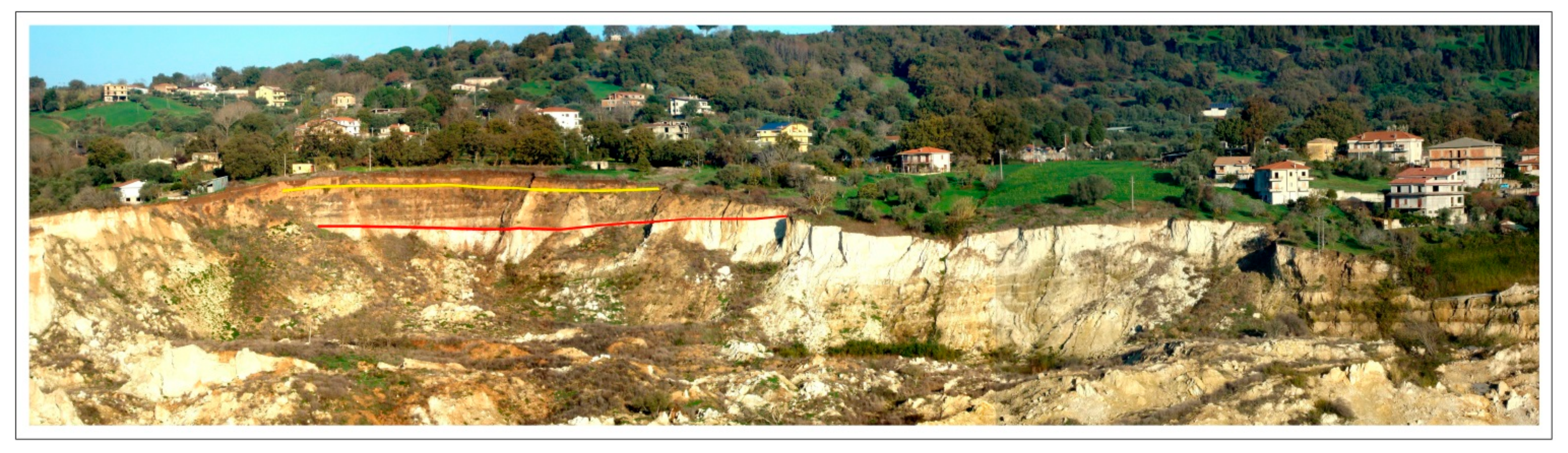
According with [25], below the vegetal soil, we can observe (from top to bottom) the following rock strata (Figure 2): (1) Pleistocene eluvio-colluvial deposits of a typical red color with a thicknesses of 0–10 m; (2) Middle Pliocene deposits of a light grey or brown color with a thicknesses of 5–25 m; (3) highly porous Upper Miocene evaporitic limestone, with a thicknesses varying between 25 and 45 m. The rock strata reduce in thickness to the west.
Taking into account the above described composition, and the interpretations of lithology and stratigraphy from borehole data [29], we can evaluate that the soil in the landslide zone has the following characteristics [30,31]: thermal conductivity k = 1.0 [W/m K], density ρ = 1600 [kg/m3], heat capacity c = 1100 [J/kg K].
2.2. The Total Station Monitoring: Layout and Instruments
Landslide monitoring using total station is generally performed by using three components: (1) a reference network materialized with prisms fixed in a stable position that can be observed from the instrument, (2) one or more stations established on stable ground at locations from which the landslide surface is visible, (3) a group of monitoring prisms at the likely unstable slope zone or area of interest.
By following the suggestions of the geologists, a permanent station was installed on a balcony of a building, located on the opposite side of the landslide, from which it is possible to observe almost the entire crown of the landslide and the town (Figure 3). The permanent station is positioned on the right side of the Scotrapiti ditch, near the border but outside the DSGSD. Two points, outside the landslide area and visible from the total station, are used for referencing aims and to control global movements. These reference points are periodically surveyed by GNSS receivers. The stability of the station was confirmed by the data collected by a Topcon GPT-8003 total station, which had operated in the same location for eight months after the failure stage.
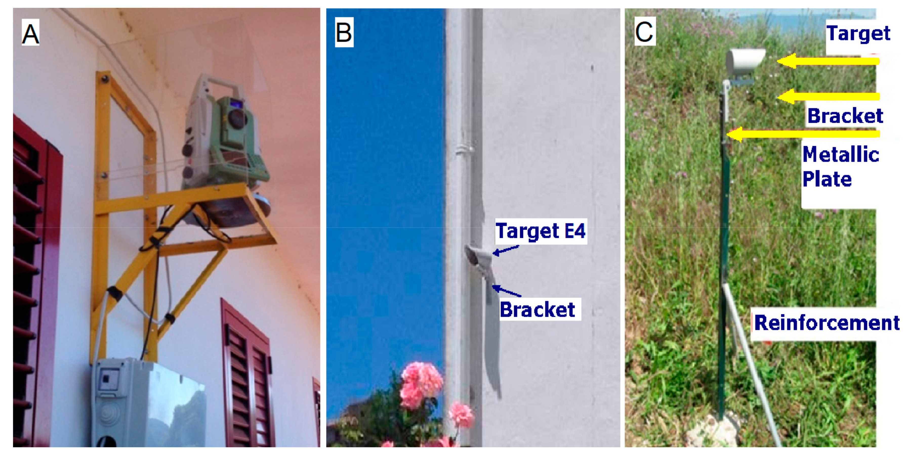
The topographic monitoring of the landslide involves 20 points, 12 of which are located along the crown and eight on some surrounding buildings. On each point, a cube corner prism was installed for the execution of automated measurements. Along the crown of the landslide, the prisms were positioned and installed on iron bars, about one meter in height, grounded with concrete and braced; the prisms on the walls of the surrounding buildings were fixed by raw plugs.
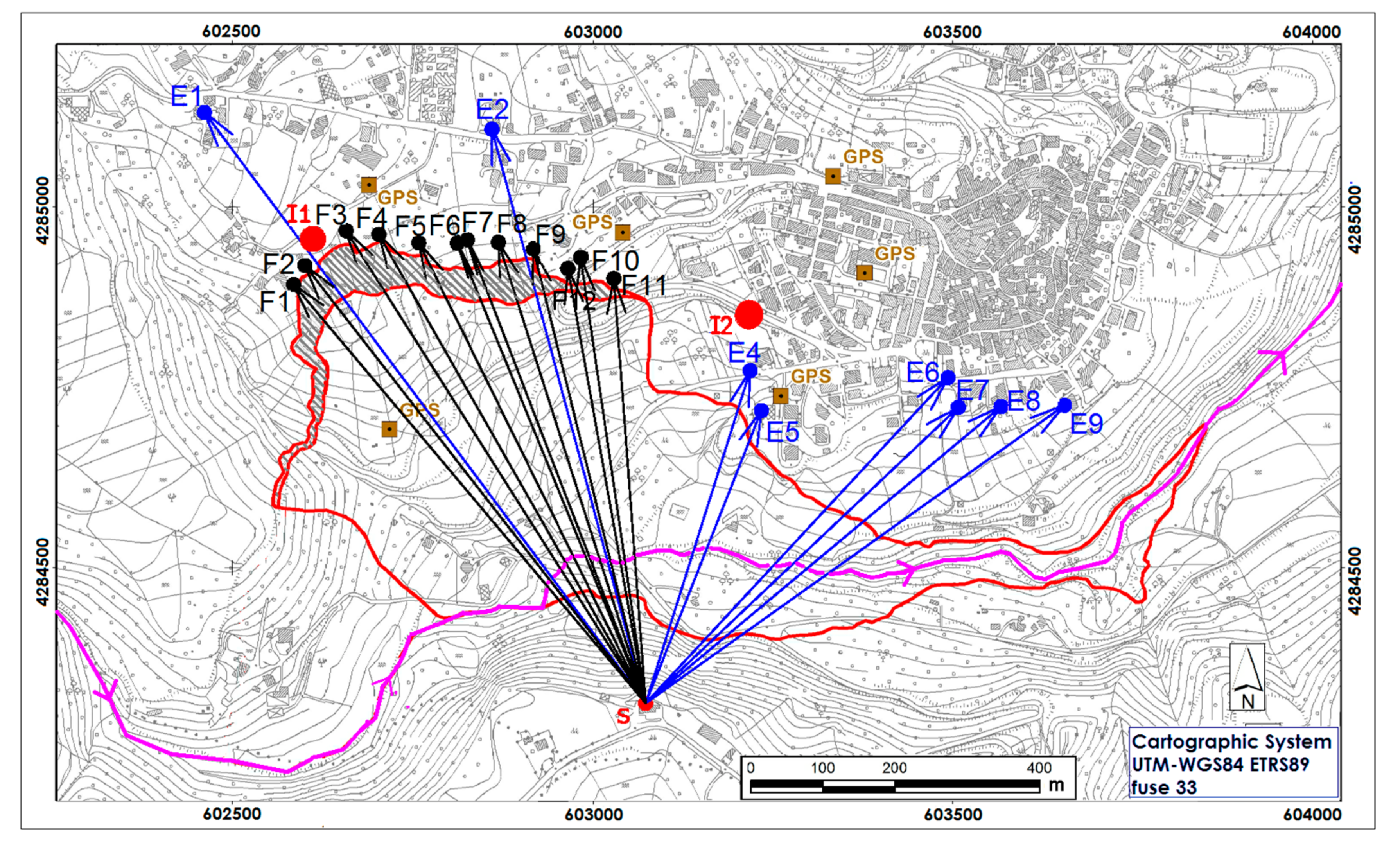
Figure 4 shows the layout of the total station monitoring; point S is the station, black points are located along the landslide crown, blue points are prisms fixed on buildings; yellow squares are points periodically surveyed by GNSS receivers, I1 and I2 are two boreholes which house inclinometers. In accordance with the geologists’ indications, a prism was positioned on a building, one km away, to have a stable reference (point E1). A second stable point E2, facing the same side of the monitored buildings, is used as control point, to evaluate the stability and effectiveness of the total station.
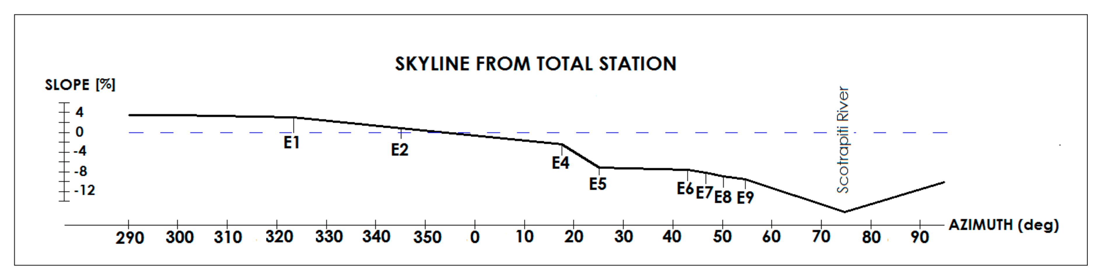
Figure 5 shows the skyline observed from the total station: we can see that the height declines to the Scotrapiti River. This is confirmed by the present cross-sections shown in Figure 6, where the distances and the heights on the left side are referred to the total station, while the dashed line is horizontal.
For the continuous monitoring, a total station Leica TS30 was used, connected to a panel for the remote control and for data exchange. The instrument was positioned on a support consisting of an iron bracket specially designed, which was affixed on a wall of the building. For the protection against wind and rain, the bracket is equipped with a Plexiglas cover, which does not interfere with the measurements. The main characteristics of the total station are summarized in Table 1.
The panel for remote control and data exchange houses: (1) a processing unit; (2) a data transmission module; (3) a device for electrical protection; (4) a switch-box controllable remotely for the restart of the total station in case of malfunction; and (5) an uninterruptible power supply to ensure proper functioning in the absence of electrical network for a time varying from 3 to 6 h.
A weather station was positioned close to the total station; it allows to obtain atmospheric parameters (pressure, relative humidity, and temperature). All measurements are performed every 20 min and data is sent to the Geomatics Lab of the University of Calabria for processing.
2.3. Analysis of the First Results
In order to fully utilize the performances of EDM, the atmospheric parameters obtained by our weather station are used. The refractive index of air can be obtained by using known models [15], [32]. In our case, to correct the EDM measurements for the atmospheric effects, the following formula [18] based on the Barrel and Sears model [33] and obtained for a wavelength of 658 nm was applied:
where ΔD is the atmospheric correction in parts per million (ppm), p is the atmospheric pressure in mbar, hr is the relative humidity, T is the temperature in °C, α = 1/273.15 and x = (7.5T/(237.3 + T)) + 0.7857.
Given a raw measure Draw, the weather corrected distance Dc is therefore:
Taking into account the climatic data provided by the Regional Agency for the Environment of Calabria Region [34], it is reasonable to adopt the same values for atmospheric pressure and a variation of the relative humidity less than 15% along the path followed by the EDM laser beam in the whole landslide area; in this case, we obtain a correction of almost 1 ppm per degree of temperature increment. A commonly used procedure takes advantage of the use of some stable points well distributed, but in our case we cannot consider stable points in the town and on the left flank of the landslide; in this way, the only reference points could be E1 and E2, decentered with respect to the others.
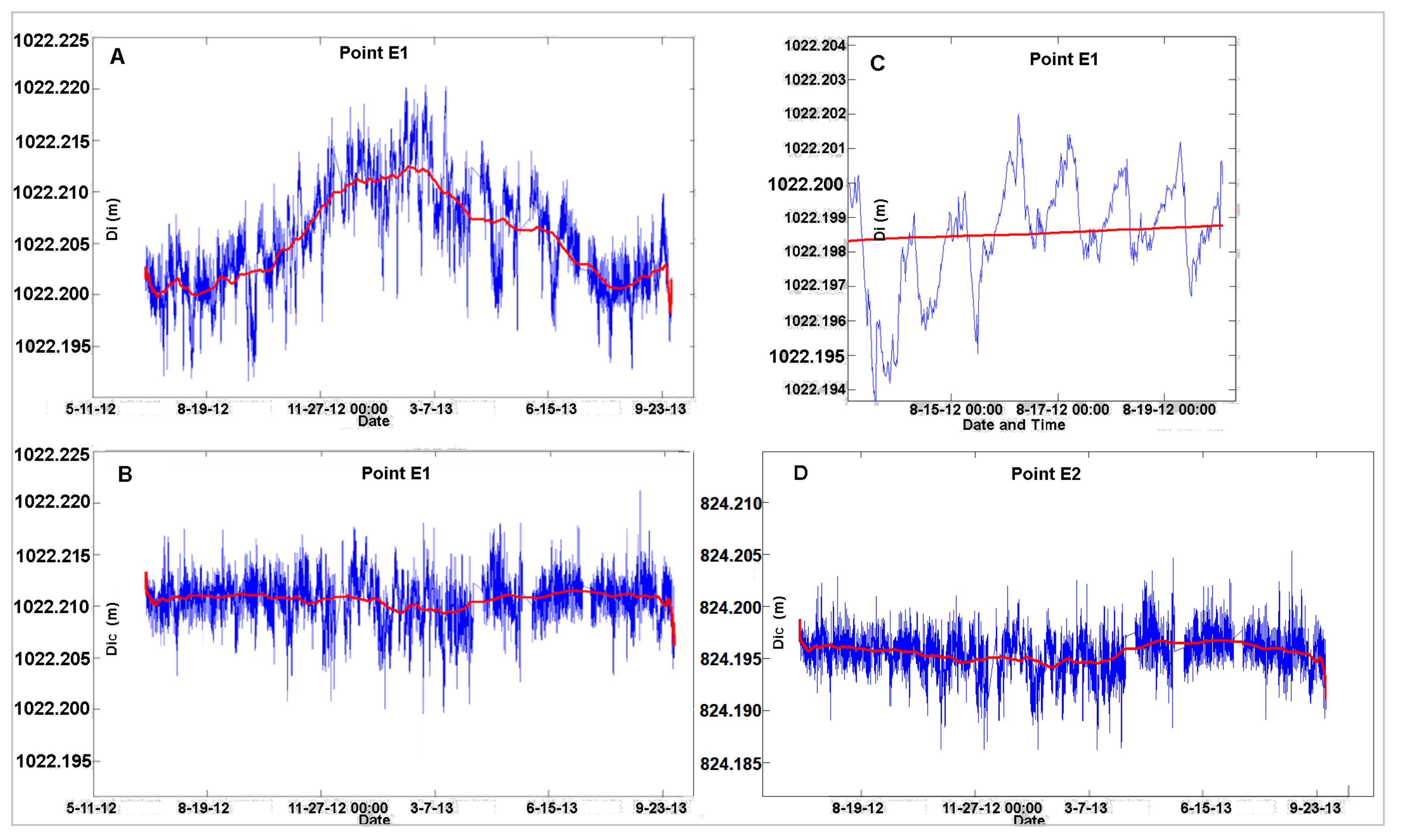
Figure 7A shows the raw values of the slope distance from station to E1. The red lines represent the results after the application of a 300-point (four days) moving average filter. Figure 7B,D shows the slope distances from station to E1 and E2 after applying Formula (2). Figure 7C is an enlargement of Figure 7A. We can observe the same oscillations of the results: actually, the terrain cross sections are very similar. Thus E1 was chosen as reference point and E2 as control point.
To calibrate the monitoring system, the average weather corrected value obtained for the first year of acquisition for point E1 was computed and was chosen as reference value. Following the procedure, for every measure, the residual is transformed in part per million (ppm) of the distance:
where D1raw is the raw distance to E1 and D1fix is the reference value.
The correction is then applied to the other measured distances; therefore, the corrected distances Dj are:
where Djraw is the raw measure from total station to target j.
A similar method can be applied to obtain the correction of the vertical angles, used for height measurement [26].
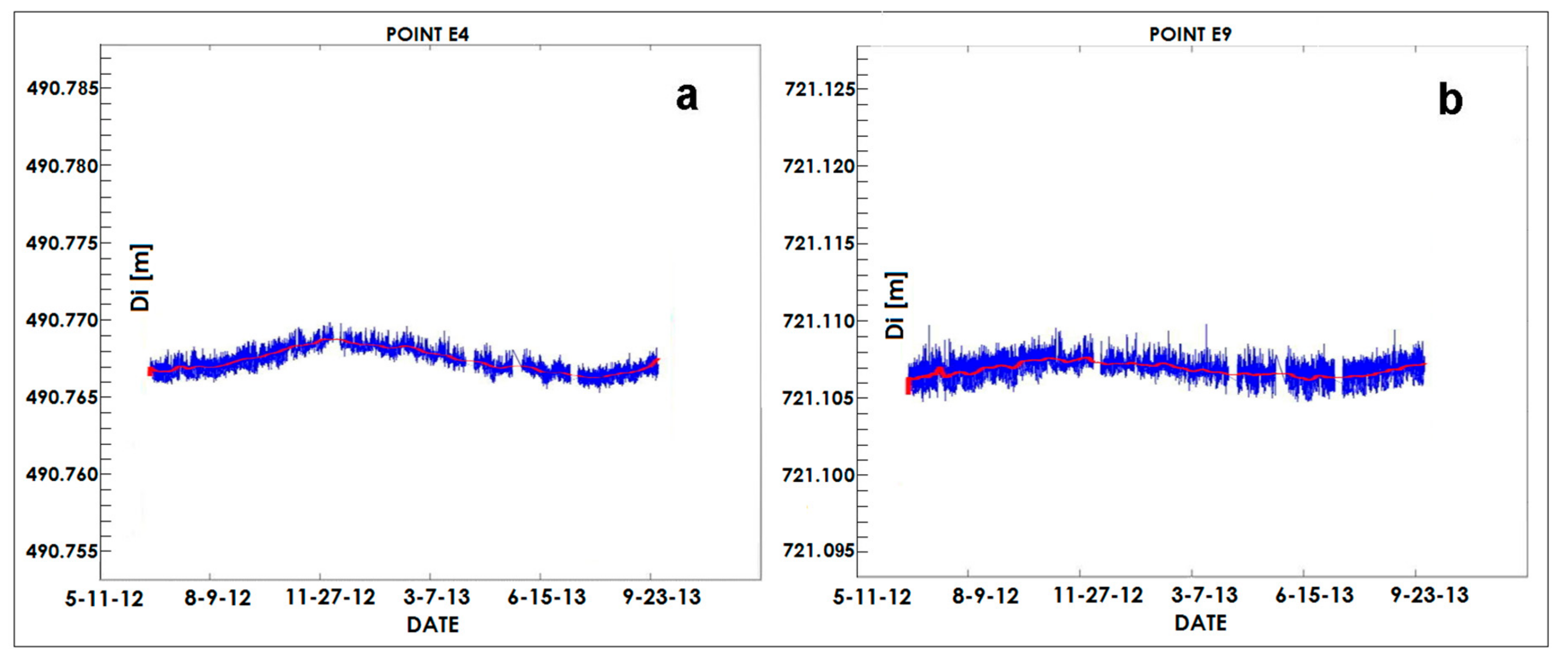
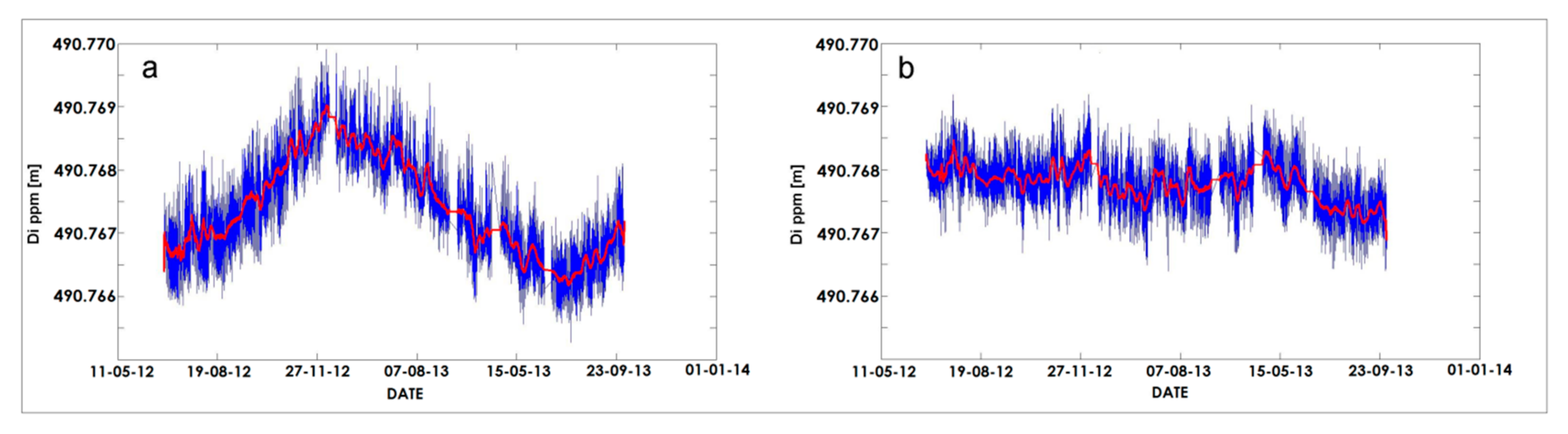
Figure 8 shows the slope distance from station to point E4 (a) and E9 (b) after applying the correction in ppm obtained by assuming fixed the distance to E1. Despite the correction, we can observe both short and long term fluctuations. Short oscillations have an identical behavior: the average amplitude is equal to ±0.7 mm for E4 (1.4 ppm) and to ±1 mm for E9 (1.4 ppm). Long term fluctuations are quite different. If we consider the smoothed values (red lines) we can observe that the amplitude is equal to ±1.3 mm for E4 (1.8 ppm) and to ±0.6 mm for E9 (0.8 ppm).
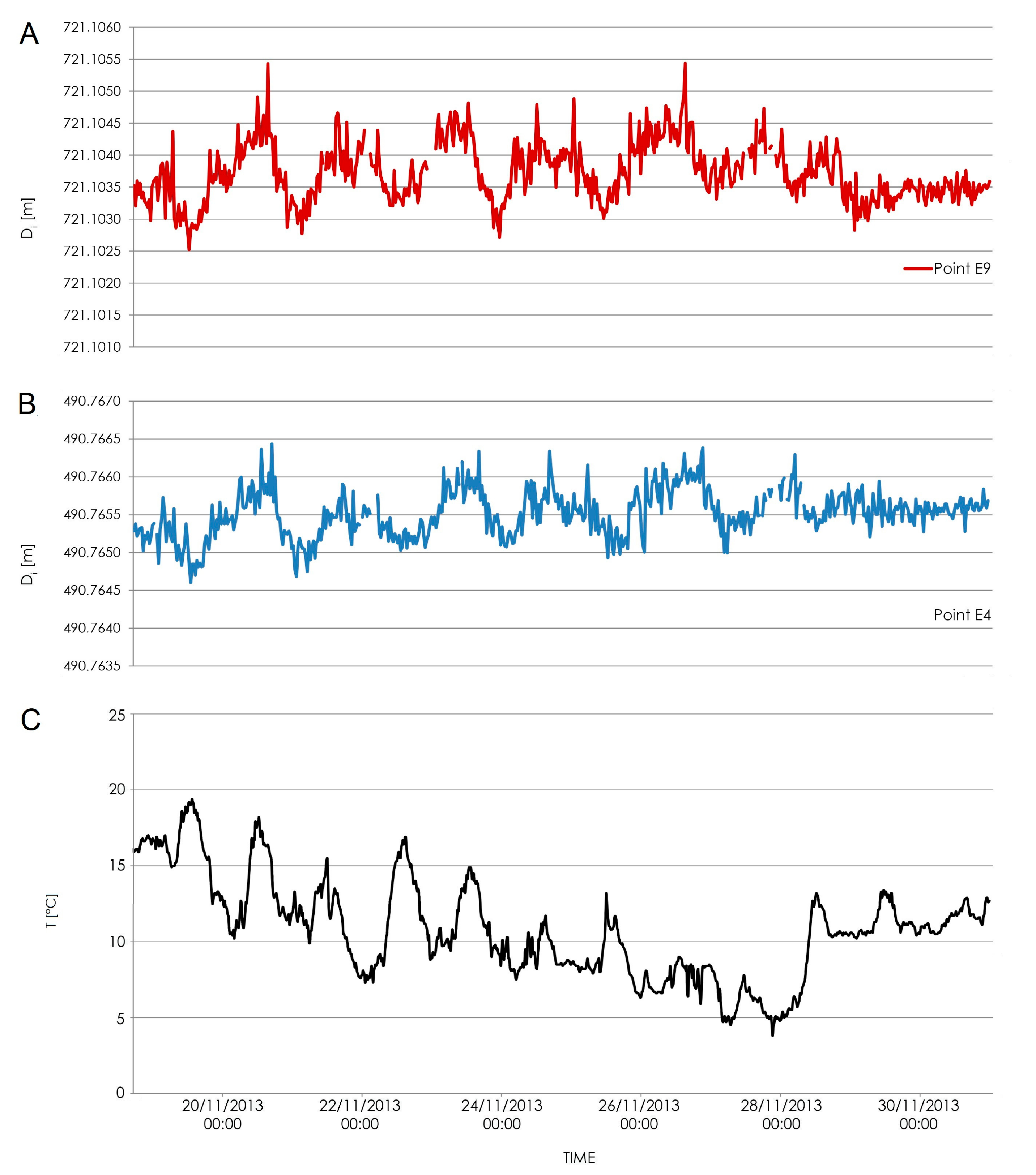
Figure 9 shows the daily temperature variations and the slope distance from station to point E9. We can observe that the amplitude of the short oscillations is correlated to the daily temperature ranges.
Figure 10 shows the temperature and the distances obtained, for a 10 days period, for targets E4 and E9.
The nearly linear relation between amplitude of short oscillations and daily temperature range is shown in Figure 11 for points E4, E5 and E9. The regression coefficients are 0.137 for E4, 0.140 for E5 and 0.147 for E9. For the whole data, the regression coefficient is equal to 0.141 ppm/°C.
To obtain quantitative values for the period of short and long term fluctuations, we applied Fast Fourier Transform to the values obtained after applying the correction in ppm derived by assuming fixed the distance to E1. In this way, the searched periods have been detected, corresponding to the annual and daily oscillations: a first peak is obtained for the frequency of 3.307 × 10⁻⁸ Hz, corresponding to a period of about 350 days; a second peak is detected for the frequency 1.159 × 10⁻⁵ Hz, which corresponding period is 24 h.
The analysis of the results obtained after applying the correction derived by fixing the distance of target E1, suggests the following remarks: (1) After the correction, the distances show both annual and daily oscillations, almost sinusoidal; this is confirmed by the results of the Fast Fourier Transform; (2) The amplitude of the annual oscillations is maximum for target E4, it decreases in the east, almost following the skyline as seen from the station; (3) An offset of about three months can be detected between maximum values of annual oscillations and equinoxes; (4) It is possible to observe a correlation between the oscillation of the distances and the daily temperature ranges; their ratio is almost constant and equal to 0.14 ppm/°C. The beginning of the daily oscillation is at 20 o’clock.
The methods based on distance ratios and/or local scale parameters work best when all trajectories connecting the total station to the monitored point’s lines have similar longitudinal profiles. This is not true in general. In our case, the use of the distance ratios introduces a time varying error because of the final 25–30% of the measurement line S-E1 which runs close and almost parallel to the ground which is not the case for the monitoring sites E4 to E9. Furthermore, the daily temperature variations are probably connected to wind and total irradiance variations during the day, which drives the amount of error introduced by the final portion of S-E1. The highly time-varying component of the atmospheric effects is taken into account by the only local scale factor (and for this aim the current meteo measurements are not needed), the spatial variability mainly depends on height above ground because the soil/surface is very homogeneous, humidity variations are negligible because of relatively dry air and/or low temperatures, and the difference between temperature close to the ground and up to 80 m above ground is well reflected by the assumed soil radiation model and by the logarithmic temperature variation with height.
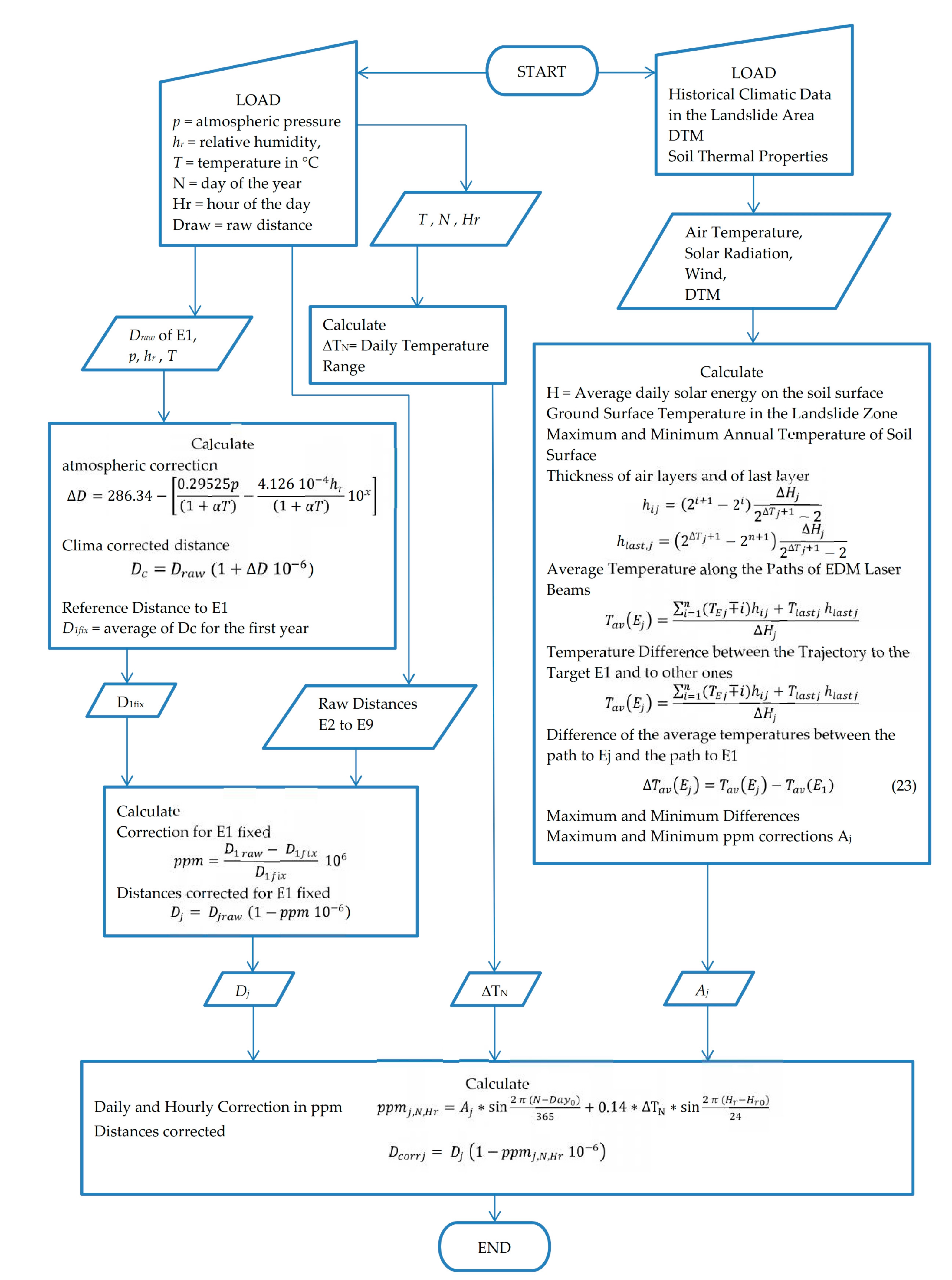
The previous considerations suggest a methodology for improving the accuracy of measurements, by using a temperature model derived by taking into account the geometric characteristics of the landslide, with a peculiar attention to the DTM. Figure 12 shows the flow chart of the proposed algorithm.
Starting with the climatic data, the solar radiation values on a horizontal surface and by using a 3D TIN model, the average daily solar energy incident on the ground in the landslide area is computed. A computer code allows to model the ground surface temperature in the landslide zone. The maximum and minimum temperatures are then obtained for each month.
Once computed the maximum and minimum annual temperatures on the soil surface, and by taking into account a convective heat transfer coefficient depending on the laser beam azimuth, the layering of the air temperature in the landslide zone is obtained. The average temperatures along the trajectories connecting the total station to the monitored points are then computed, along with the maximum and minimum ppm corrections. For all trajectories, day by day and hour by hour, the ppm corrections are computed, by using a sinusoidal variation and the daily temperature ranges. These corrections are applied to the distances previously modified using the correction in ppm obtained by assuming fixed the distance to E1.
To apply the proposed methodology, the ground surface temperature and the layering of the air temperature must be obtained.
2.4. The Solar Radiation in the Landslide
Solar radiation and air temperature, as well as wind and rain, are the most important meteorological factors that influence the surface and subsurface temperature [19]. The heat exchange between the atmosphere and the ground depends also on vegetation and on geometric characteristics of the terrain. Slope orientation and inclination determine the angle between solar rays and normal to the surface and, consequently, the amount of solar power incident on the ground and the net radiation balance [35].
Below the ground surface, almost all thermal energy is transferred by conduction; thus the most important properties to use are heat capacity, thermal conductivity and soil latent heat [36,37]. The wind speed is the most important information for modeling the convection heat transfer between air and ground and between air layers. The effect of evaporation may not be considered in our case, given that there is no vegetation in the landslide.
Electromagnetic radiation is the most important factor in the total energy budget. During the day, the shortwave radiation, due to the sun, is dominant, and the incoming energy, for a lightened surface, is higher than the outgoing one; at night the energy balance is dominated by long-wave radiation [19] and the outgoing energy, most of all in clear nights and in absence of dense vegetation, is greater than the incoming one.
The values of the main atmospheric parameters for the zone of Maierato are reported in Table 2.
Data are the average values of the last 40 years and was provided by the Regional Agency for the Environment of Calabria Region’s historical database [34]. It should be underlined that the values of solar energy are referred to a horizontal surface with a flat skyline; slope and the orientation of the terrain along with the shadowing due to the surrounding elements (buildings, hills, vegetation, etc.) can be taken into account by using a DTM of the landslide zone.
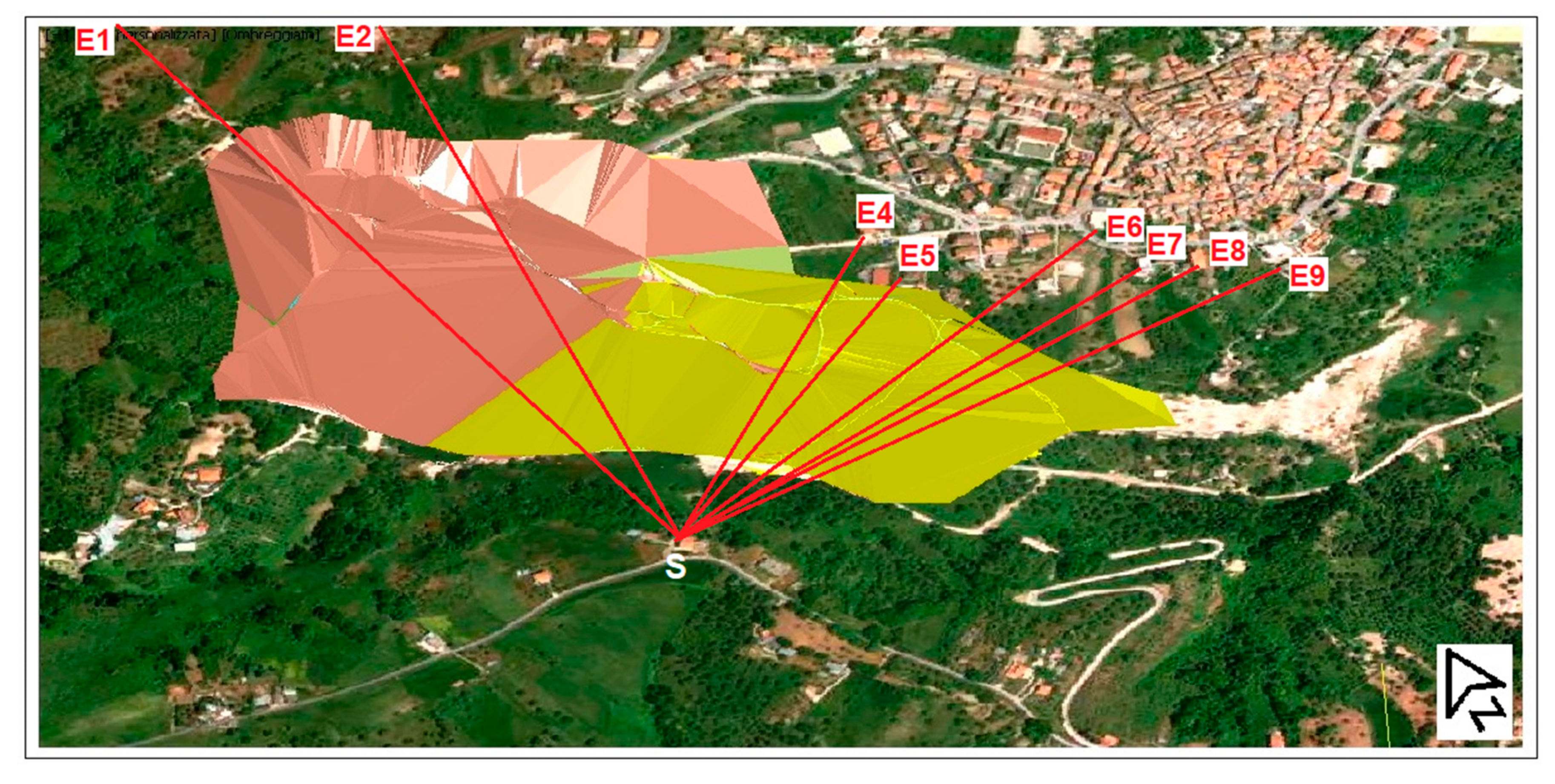
To obtain the post-failure DTM, a terrestrial laser scanner survey has been performed; the instrument used is the LMS-Z420i manufactured by RIEGL GmbH, Horn, Austria, with a measurement range of about 1000 m and an accuracy of 10 mm. Figure 13 shows the 3D model of the present situation superimposed to an aerial photo: due to the landslide, a zone in the form of a basin was created.
Among the several formulas available in literature to obtain the daily solar energy H incident on a tilted surface, we used the one suggested by UNI, the Italian Organization for Standardization [38]. The known elements are: (a) the global and the diffuse daily solar energy on a horizontal surface (Hh, Hd) attainable by Table 2, (b) the latitude ϕ of Maierato (38°42′16″ N), (c) the angle β the surface makes with the horizontal, (d) the surface azimuth γ, defined as the deviation of the projection on a horizontal plane of the normal to the surface from the local meridian, with zero due south, east negative, west positive, (e) the solar constant Go = 1,353 W/m2, (f) the sun’s declination angle δ, (g) the albedo ρ (reflection coefficient of the soil surface) that, in our case, can be considered equal to 0.2, (h) the sun hour angle at sunrise for a horizontal surface ϖs, (i) the sun hour angles at sunrise and sunset for the considered surface ϖ′ and ϖ″.
The daily solar energy H incident on a tilted surface is given by:
To obtain the coefficient R, the geometric characteristics of the area are taken into account. Topographic shading of direct radiation is accounted for and diffuse radiation is modified by the proportion of sky in view: the irradiation deficit due to shadowing is taken into account through the angles ϖ′ and ϖ″. Since in the landslide area there are not artificial shadings like in the towns, the actual sunrise and sunset times give sufficient information. Furthermore, for our aims we do not need a very detailed microclimate model, so a simplified method can be used.
Starting from the known elements, we obtain the coefficients T, U, V:
For β = 0, the coefficients Th, Uh and Vh can be obtained. The direct solar energy on the tilted surface Hb and the direct solar energy on a horizontal surface Hbh can be computed, along with the ratio Rb:
Finally, the coefficient R is given by:
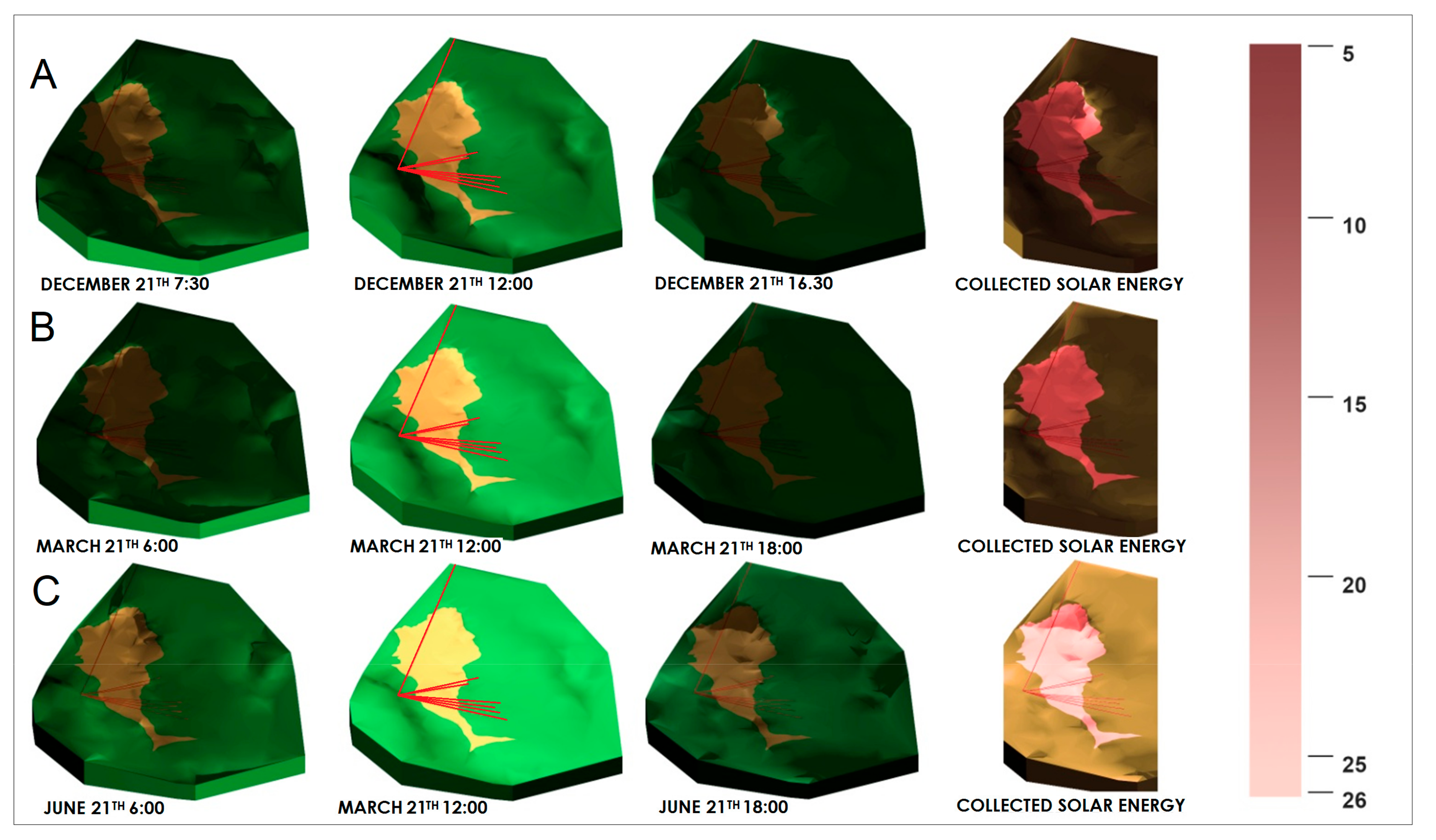
Figure 14 shows the instantaneous solar lighting in the landslide and in the surroundings and the average daily solar energy incident on the ground for different dates and times, obtained by using the data of Table 2 and the TIN model. Red lines are the paths of the EDM laser beams, starting from the station on the hill. In the first row, from left to right, we can observe the radiation incident upon the ground on 21 December, winter solstice, for different times (7:30, noon and 16:30); the light areas are lit by the sun, the dark ones are in shadow; the fourth image represents the daily solar energy collected by the ground in a color scale, ranging from 5 to 26 MJ/m2 day. In the second and third rows, the radiation and daily energy values are shown on 21 March, the vernal equinox, and on 21 June, summer solstice.
We can make the following remarks: (1) during winter, when the solar angle is minimum, the zone where the targets E4–E9 are located, gets solar energy only a few hours, due to the low sun angle and to the shading caused by the hill where the total station is positioned. The prevailing winds (SW, SE) are shielded by the same hill. Thus, the temperature on the soil and near the soil is lower than outside the landslide, during the day, due to the low solar radiation and at night (above all in clear nights) due to the long-wave radiation and the absence of wind. (2) During summer, the mentioned zone gets almost the same solar energy as the external one, due to the high sun angle. The prevailing winds (SW, NW) are shielded by the same hill and by the main scarp of the landslide. Thus, the temperature on and near the soil is higher than outside the landslide due to the greater solar energy gain in absence of vegetation and wind. (3) Furthermore, by taking into account the skyline (Figure 4) and the cross sections (Figure 5) we can observe that the shielding effect due to the hill decreases from E4 to E9 and an increasing convective heat exchange must be foreseen.
2.5. Modeling the Ground Surface Temperature in the Landslide Zone
A software program was developed by using Matlab® software and the Simulink® libraries. The calculations are based on the following parameters’ input: thermal conductivity, density, heat capacity, air temperature, relative humidity, solar radiation, and convective heat transfer coefficient. For the first three parameters, the values reported in Section 2.1 were used. The daily air temperature and the relative humidity were obtained by interpolating the values of Table 2, while the solar radiation was computed as previously described, and it was considered constant every month. During the night, the radiative cooling was taken into account. The net outgoing radiation varies from about 15 W/m2 for an overcast night, to 100 W/m2 for a clear sky night [39], so we adopted values ranging from −45 W/m2 in January (40% of clear sky nights) to −87 W/m2 in July (90% of clear sky nights). A convective heat transfer coefficient equal to 6 W/m2 · K was chosen for the calm zone; the coefficient increases with the azimuth up to 24 W/m2 · K, going from the direction to E4, to the direction to the bottom of the Scotrapiti River.
The procedure described in detail in [40] was applied. The soil model make use of two main equations for heat and moisture transfer within soil. For heat conduction the one-dimensional diffusion equation is:
where ν, cs, and ρs, are the thermal conductivity, specific heat capacity, and soil density, respectively (obtained in the section geological settings). The expression ν ρ/scs = ks is called the thermal diffusivity. In several cases, ks can be considered constant along z-axis [41]; the equation then becomes:
The vertical one-dimensional equation of diffusive and gravitational motions for soil moisture transfer is:
where Dn and Kn are diffusional and hydraulic conductivity, respectively.
The heat budget equation for the interface-spanning layer with average temperature Tg is written as:
where Rn is net radiation, H is sensible heat flux, LνE is latent heat flux, and G is soil heat flux, G = . (Radiation fluxes are defined positive toward the surface, other fluxes positive away from the surface.)
The software program uses the finite difference method. The maximum and minimum temperatures have been obtained, respectively, in July and January.
2.6. Average Temperature Along the Paths of the Laser Beams and ppm Corrections
According with the literature [19], it is reasonable to hypothesize that the air temperature varies with the height in a binary logarithm way. Thus, for our simulation, we can consider air layers starting from each target, characterized by an average difference of temperature of one °C and by doubled thicknesses.
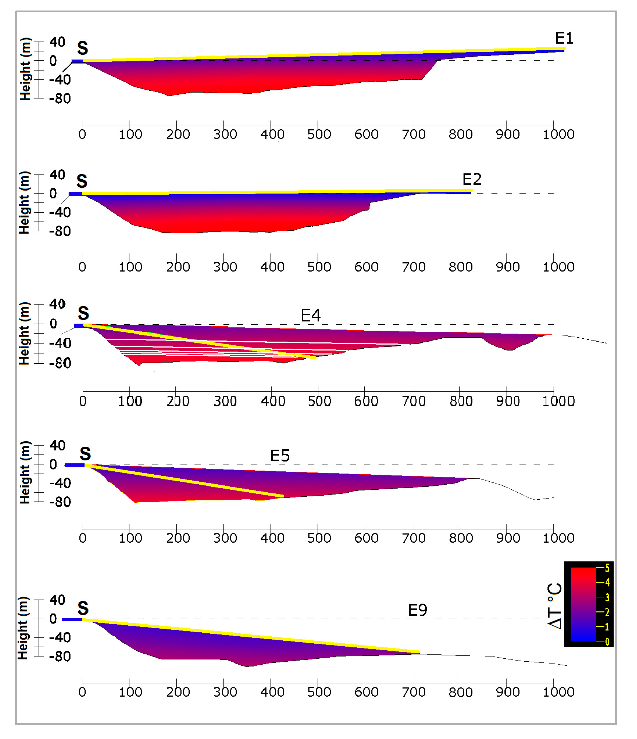
Figure 15 shows, in a range of colors, the difference between air temperatures in the landslide zone and external air temperature calculated for July. The values range from 0 °C (blue) to 5 °C (red). The heights on the left side refer to the total station S, the dashed line is the horizontal, the yellow line is the EDM laser beam path. For target E4, the layers are shown, separated by white lines.
To obtain the height of the layers, we use the following procedure. We define:
ΔTj = temperature difference between the target Ej and the total station;
ΔHj = height difference between the target Ej and the total station;
n = the integer part of ΔTj;
We divide the atmosphere between each target and the total station into n + 1 layers.
For the thickness of the ith layer of the jth trajectory (starting from the soil and for i = 1 to n), we can state the proportionality:
For the thickness of the last layer we can write:
The total thickness, equal to the height difference between the target Ej and the total station, is:
The thickness of the ith layer is given by:
The thickness of the last layer is:
If we neglect the curvature of the laser beam of EDM, the path from the total station to the target Ej can be divided in n + 1 segments, whose lengths are directly proportional to the thickness of the relevant layer. The average temperature of the atmosphere along a laser beam path is then given by:
where TEj is the temperature of the air at the point Ej. The difference of the average temperatures between the path to Ej and the path to E1 is given by:
Actually, the air layers close to the ground follow the topography. Thus, for each layer, the length of the beam path depends not only on the thickness, but also on its angle of incidence, that has been neglected in our model. Nevertheless, this simplification is justified if we consider that: (a) even for the lower layers, the separation surfaces are roughly horizontal in most cases; (b) the lower layers have a very limited thickness compared to the higher ones. Therefore, a more accurate modeling of the laser beam path could be requested just for critical conditions, e.g., for a signal path almost parallel to a very steep slope.
As stated in Section 2.3, it is reasonable to consider a correction of 1 ppm per degree of temperature difference. The absolute values of maximum correction Aj (in ppm), obtained with the procedure described previously, are reported in Table 3. The values range from 2.10 for the target E4, to 0.65 for the target E9.
If we do not consider the daily oscillation of air temperature, the correction for the slope distance is sinusoidal and it ranges between the values Aj and −Aj, given by Table 3 for each target. Given that the annual oscillations begin around 15 September (close to the fall equinox), the correction for the Nth day of the year, expressed in ppm, is given by:
where: Aj = maximum absolute value of ppm correction of the slope distance from total station to Ej; N = day of the year; Day0 = day of the beginning of the yearly oscillation (258 = 15 September).
Taking into account the daily ranges of air temperature and the correlation described in Section 2.3, the correction for the slope distance, for the Hth hour of the Nth day of the year, expressed in ppm, is given by:
where: Hr = hour of the day; Hr0 = 20, hour of the beginning of the daily oscillation; ΔTN = temperature range of Nth day.
The distances corrected are:
2.7. The Atmospheric Correction of the EDM Measurements
To obtain the atmospheric correction for the EDM measurements, the following steps are followed: (a) We compute the maximum and minimum annual temperatures on the soil surface, by taking into account low-medium values of the ground thermal diffusivity and a convective heat transfer coefficient, which depends on the laser beam azimuth; (b) We consider calm air and the stratification described in Section 2.6; (c) Taking into account the maximum and minimum temperatures of the soil surface, we compute the average temperatures along the trajectories connecting the total station to the target E1 and to targets E4–E9 using Equation (22); (d) We calculate the maximum and minimum temperature differences between the trajectory to E1 and the trajectories to E4–E9 using Equation (23) and, consequently, the relevant maximum and minimum ppm corrections; (e) For all trajectories we compute, day by day and hour by hour, the ppm corrections using Equations (24) and (25). We compute distances corrected using Equation (26).
Figure 16 shows the corrections, expressed in ppm, of the slope distances, computed for target E4. In Figure 16a the corrections for the whole monitoring period are represented; in Figure 16b the corrections for a period of 30 days, circled in red in Figure 13a, are shown, along with the daily range of external air temperature.
3. Results and Discussion
In the following, we can observe a comparison between the results obtained by applying the corrections in ppm deduced by fixing the distance to E1, and the results obtained by adopting the methodology previously described. The procedure has been applied to the measurements carried out over a 15 month period, from June 2012 to September 2013, during which over 38,000 distances have been acquired for each target.
Figure 17 shows the results obtained for target E4 (a,b); the red lines represent the results after the application of a 300-point moving average filter. The values of slope distances for the whole monitoring period are shown; some power failures caused the loss of measurements for short periods, easily detectable in the graphs. On the left we can see the results of applying the corrections in ppm obtained by fixing the distance E1: the residual seasonal oscillations are noticeable. On the right the distances obtained by adopting the methodology described in Section 2.6 are shown; two results have been obtained: (1) the long term oscillations are almost eliminated; (2) the range between maximum and minimum values is dramatically reduced.
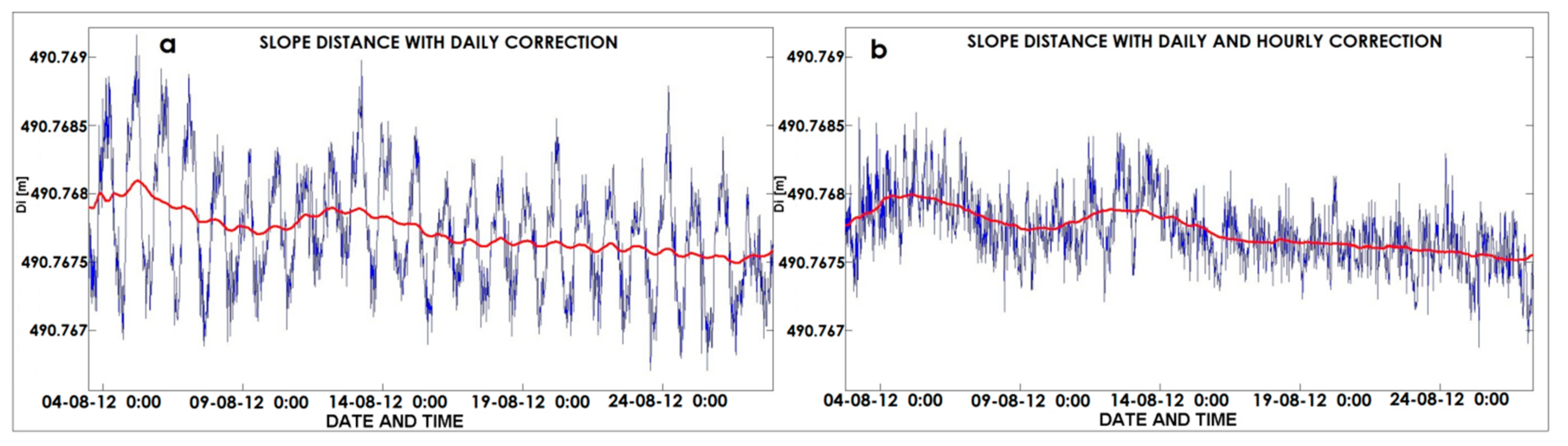
Figure 18 shows the results obtained from 4 to 28 December 2012 for the target E4, by applying only the daily correction (a) and once applied both daily and hourly corrections (b). Three considerations can be made: (1) daily oscillations are reduced; (2) the lines drawn by using a 300 point moving average filter (red lines) are further smoothed; and (3) the range of the residual measurement noises is drastically reduced.
The overall results obtained during the whole monitoring period for each target are summarized in Table 4, where: Di is the average slope distance in m; σraw is the standard deviation of the raw acquisitions in mm; σtemp is the standard deviation of the distances obtained by using Equation (1) and the atmospheric data collected by the weather station; σE1 is the standard deviation of the distances with the corrections in ppm obtained by fixing the distance to the target E1; σtot is the standard deviation of the distances obtained by adopting the described methodology; Declared EDM accuracy is the value of accuracy, at 95% confidence level, which can be expected in ideal conditions, according to the characteristics declared by the manufacturer and reported in Table 1 (0.6 mm + 1 ppm).
We can underline the progressive reduction of the standard deviation. By using the atmospheric data acquired by the weather station, the reduction is about 60%. A further reduction is obtained by fixing the distance to target E1; the improvement is less for the targets E4 and E5, which are more influenced by the layering of the air in the landslide area. By using the method described in the paper, we obtained the best results and the influence of the microclimate is almost corrected: the reduction of the standard deviation is about 90%, while the final standard deviation is about proportional to the distances and does not depend on the directions. In the last column we report the accuracy, at 95% confidence level, which can be expected in ideal conditions, according to the characteristics declared by the manufacturer (Table 1): we can observe that these values are almost equal to 2σtot; this confirms the effectiveness of the described methodology.
The fluctuation of the results that still remain even after the application of the proposed methodology is probably due to changes in the parameters not considered in the model. In any case, the effects of these variations are less than the stated accuracy for the total station used, so a more sophisticated model might not be very useful.
With reference to the usability and feasibility, the method is more effective when the longitudinal profiles along the trajectories connecting the total station to the monitored points are different, which can produce different meteo-climatic parameters (wind, temperature range). We observe that the methodology presented could be largely adopted with very low costs. In fact, the requested information is a DTM, along with historical climatic data. Given that the same robotic stations used for monitoring can perform automatic scanning and the recent EDMs can measure ranges up to 2000 m without targets, a DTM can be obtained easily and inexpensively. The historical climatic data can be easily found in the websites of public and private institutions.
4. Conclusions
A method for the removal of the errors due to the influence of microclimate in the monitoring of a large landslide by a high-end total station has been described. The method is based on the realization of an atmospheric model by using climatic data and the DTM of the landslide area. The novel aspect of the study lies in the possibility to obtain high EDM accuracy without the necessity to install several weather stations distributed in the whole landslide area.
The methodology has been applied to the large landslide at Maierato, southern Italy. The results of the test carried out demonstrate the effectiveness of the method. The standard deviations show a reduction, ranging from 20% to 50%, with respect to the results obtained by using the most diffused procedures, still affected by both long and short term oscillations. The more evident improvements are obtained for the points situated inside the landslide zone, characterized by a basin shape. The obtained standard deviations are is in line with the values declared by the manufacturer for measurements in optimal conditions. The methodology presented could be largely adopted, above all when high accuracies are requested (monitoring of structures, cliffs, etc.), with a low cost.
Acknowledgments
The authors would like to thank Giuseppe Artese for his comments and suggestions.
Author Contributions
Serena Artese conceived the methodology and wrote the paper. Michele Perrelli realized the control panel. Serena Artese and Michele Perrelli designed the monitoring layout and performed the data processing.
Conflicts of Interest
The authors declare no conflict of interest.
References
- Kasperski, J.; Delacourt, C.; Allemand, P.; Potherat, P.; Jaud, M.; Varrel, E. Application of a Terrestrial Laser Scanner (TLS) to the Study of the Séchilienne Landslide (Isère, France). Remote Sens. 2010, 2, 2785–2802. [Google Scholar] [CrossRef]
- Lichun, S.; Wang, X.; Zhao, D.; Qu, J. Application of 3D laser scanner for monitoring of landslide hazards. Int. Arch. Photogramm. Remote Sens. 2008, 37, 277–281. [Google Scholar]
- Mallet, C.; Bretar, F. Full-waveform topographic Lidar: State-of-the-art. ISPRS J. Photogramm. Remote Sens. 2009, 64, 1–16. [Google Scholar] [CrossRef]
- Kimura, H.; Yamaguchi, Y. Detection of Landslide Areas Using Satellite Radar Interferometry. Photogramm Eng. Remote Sens. 2000, 66, 337–344. [Google Scholar]
- Tarchia, D.; Casagli, N.; Fanti, R.; Leva, D.; Luzic, G.; Pasuto, A.; Pieraccini, M.; Silvano, S. Landslide monitoring by using ground-based SAR interferometry: An example of application to the Tessina landslide in Italy. Eng. Geol. 2003, 68, 15–30. [Google Scholar] [CrossRef]
- Glabsch, J.; Heunecke, O.; Schuhbäck, S. Monitoring the Hornbergl landslide using a recently developed low cost GNSS sensor network. J. Appl. Geod. 2009, 3, 179–192. [Google Scholar] [CrossRef]
- Artese, G.; Perrelli, M.; Artese, S.; Meduri, S.; Brogno, N. POIS, a Low Cost Tilt and Position Sensor: Design and First Tests. Sensors 2015, 15, 10806–10824. [Google Scholar] [CrossRef] [PubMed]
- Afeni, T.B.; Cawood, F.T. Slope Monitoring using Total Station: What are the Challenges and How Should These be Mitigated? S. Afr. J. Geomat. 2013, 2, 41–53. [Google Scholar]
- Stiros, S.C.; Vichas, C.; Skourtis, C. Landslide Monitoring Based on Geodetically Derived Distance Changes. J. Surv. Eng. 2004, 130, 156–162. [Google Scholar] [CrossRef]
- Tsaia, Z.; Youa, G.J.Y.; Leea, H.Y.; Chiub, Y.J. Use of a total station to monitor post-failure sediment yields in landslide sites of the Shihmen reservoir watershed. Geomorphology 2012, 139–140, 438–451. [Google Scholar] [CrossRef]
- Corsini, A.; Castagnetti, C.; Bertacchini, E.; Rivola, R.; Ronchetti, F.; Capra, A. Integrating airborne and multi-temporal long-range terrestrial laser scanning with total station measurements for mapping and monitoring a compound slow moving rock slide. Earth Surf. Process. Landf. 2013, 38, 1330–1338. [Google Scholar] [CrossRef]
- Castagnetti, C.; Bertacchini, E.; Corsini, A.; Capra, A. Multi-sensors integrated system for landslide monitoring: Critical issues in system setup and data management. Eur. J. Remote Sens. 2013, 46, 104–124. [Google Scholar] [CrossRef]
- Simeoni, L.; Ferro, E.; Tombolato, S. Reliability of Field Measurements of Displacements in Two Cases of Viaduct-Extremely Slow Landslide Interactions. Eng. Geol. Soc. Territ. 2015, 2, 125–128. [Google Scholar]
- Edlen, B. The refractive index of air. Metrologia 1966, 2, 71–80. [Google Scholar] [CrossRef]
- Ciddor, P.E. Refractive index of air: New equations for the visible and near infrared. Appl. Opt. 1996, 35, 1566–1573. [Google Scholar] [CrossRef] [PubMed]
- Rüeger, J.M. Electronic Distance Measurement—An Introduction, 4th ed.; Springer: Berlin/Heidelberg, Germany; New York, NY, USA, 1996. [Google Scholar]
- Bayoud Fadi, A. Leica’s Pinpoint EDM Technology with Modified Signal Processing and Novel Optomechanical Features. In Proceedings of the XXIII FIG Meeting, Munich, German, 8–13 October 2006; pp. 1–16. [Google Scholar]
- Leica TS30/TM30 Manual 3.0. Available online: http://www.surveyteq.com/pdf/Leica_TS30_TM30_ UM_en.pdf 1.1 (accessed on 6 January 2015).
- Geiger, R.; Aron, R.H.; Todhunter, P. The Climate near the Ground, 6th ed.; Rowman & Littlefiel Publishers: Oxford, UK, 2003; p. 589. [Google Scholar]
- Brunner, F.K.; Rüeger, J.M. Theory of the local scale parameter method for EDM. Bull. Géod. 1992, 66, 355–364. [Google Scholar] [CrossRef]
- Graczka, G. The global and local scale deviations of geodetic networks observed by electromagnetic wave propagation in real atmosphere. Periodica Polytech. Ser. Civ. Eng. 1996, 40, 3–14. [Google Scholar]
- Archbold, M.J.; Mckee, C.O.; Talai, B.; Mori, J.; De Saint Ours, P. Electronic Distance Measuring Network Monitoring during the Rabaul Seismicity/Deformational Crisis of 1983–1985. J. Geophys. Res. 1988, 93, 12123–12136. [Google Scholar] [CrossRef]
- Guerricchio, A.; Fortunato, G.; Guglielmo, E.A.; Ponte, M.; Simeone, V. Hydrogeological conditioning and deep-seated gravitational slope deformations effects on the activation of the large landslide of Maierato in 2010. Tec. Dif. Dall’Inquin. 2010, 31, 661–706. [Google Scholar]
- Guerricchio, A.; Doglioni, A.; Fortunato, G.; Galeandro, A.; Guglielmo, E.; Versace, P.; Simeone, V. Landslide hazard connected to deep seated gravitational slope deformations and prolonged rainfall: Maierato landslide case history. Soc. Geol. Ital. 2012, 21, 574–576. [Google Scholar]
- Gattinoni, P.; Scesi, L.; Arieni, L.; Canavesi, M. The February 2010 large landslide at Maierato, Vibo Valentia, Southern Italy. Landslides 2012, 9, 255–261. [Google Scholar] [CrossRef]
- Artese, G.; Perrelli, M.; Artese, S.; Manieri, F. Geomatics activities for monitoring the large landslide of Maierato, Italy. Appl. Geomat. 2014. [Google Scholar] [CrossRef]
- Artese, G.; Perrelli, M.; Artese, S.; Manieri, F.; Principato, F. The contribute of geomatics for monitoring the great landslide of Maierato, Italy. Int. Arch. Photogramm. Remote Sens. Spat. Inf. Sci. 2013, XL-5/W3, 15–20. [Google Scholar] [CrossRef]
- Geologic Map of Italy Foglio 241–Settore III SE–Tavoletta “Vibo Valentia” della Carta Geologica della Calabria, Cassa per il Mezzogiorno; Poligrafica & Cartevalori Ercolano: Neaples, Italy, 1968.
- Conte, E. Report AM/R14/A_M5/a Studi ed Indagini Geologiche, Geotecniche, Idrologiche ed Idrauliche nel Comune di Maierato; Technique Report; Versace, P., Ed.; CAMILAB-University of Calabria: Rende, Italy, 2012. [Google Scholar]
- Ochsner, T.E.; Horton, R.; Ren, T. A new perspective on soil thermal properties. Soil Sci. Soc. Am. J. 2001, 65, 1641–1647. [Google Scholar] [CrossRef]
- Farouki, O.I. Thermal Properties of Soils; CRREL Monograph: Hanover, NH, USA, 1981; 151p. [Google Scholar]
- Ciddor, P.E.; Hill, R.J. Refractive Index of Air. 2. Group Index. Appl. Opt. 1999, 38, 1663–1667. [Google Scholar] [CrossRef] [PubMed]
- Barrell, H.; Sears, J.E. The Refraction and Dispersion of Air for the Visible Spectrum. Philos. Trans. R. Soc. Lond. 1939, 238, 1–64. [Google Scholar] [CrossRef]
- Regional Agency for the Environment of Calabria Region’s Historical Database. Available online: http://www.cfd.calabria.it/index.php?option=com_wrapper&view=wrapper&Itemid=41 (accessed on 6 January 2015).
- Bennie, J.; Huntley, B.; Wiltshire, A.; Hill, M.O.; Baxter, R. Slope, aspect and climate: Spatially explicit and implicit models of topographic microclimate in chalk grassland. Ecol. Model. 2008, 216, 47–59. [Google Scholar] [CrossRef]
- Deardorff, J.W. Efficient Prediction of Ground Surface Temperature and Moisture, With Inclusion of a Layer of Vegetation. J. Geophys. Res. 1978, 83, 1889–1903. [Google Scholar] [CrossRef]
- Tassou, P.S.; Pouloupatis, D.; Florides, G. Measurements of ground temperatures in Cyprus for ground thermal applications. Renew. Energy 2011, 36, 804–814. [Google Scholar]
- UNI. Energia Solare. Calcolo Degli Apporti per Applicazioni in Edilizia. Valutazione Dell’ Energia Raggiante Ricevuta; Norma 8477 Part 1; Italian Organization for Standardization: Milano, Italy, 1983. [Google Scholar]
- Eriksson, T.S.; Granquist, C.G. Radiative cooling computed for model atmospheres. Appl. Opt. 1982, 21, 4381–4388. [Google Scholar] [CrossRef] [PubMed]
- Smirnova, T.G.; Brown, J.M.; Benjamin, S.G. Performance of Different Soil Model Configurations in Simulating Ground Surface Temperature and Surface Fluxes. Mon. Weather Rev. 1997, 125, 1870–1884. [Google Scholar] [CrossRef]
- Bellecci, C.; Artese, G.; Greco, M.R.; Zupo, M.S. Ground as a Thermal Buffer for Building Climatization: How to Recharge It. Proc. ISES Sol. World Congr. Bp. 1993, 6, 381–386. [Google Scholar]
Figure 1.
(a) The map of Southern Italy. The red circle indicates the location of Maierato (38°42′16″ N, 16°11′01″ E). (b) The Maierato Landslide area. The red line is the main scarp of the DSGSD, the yellow line is the contour of the landslide, the pink line is the Scotrapiti ditch, which constitutes the SW border of the DSGSD, and the blue line is the Ceramida ditch. The arrows indicate the direction of the watercourses.
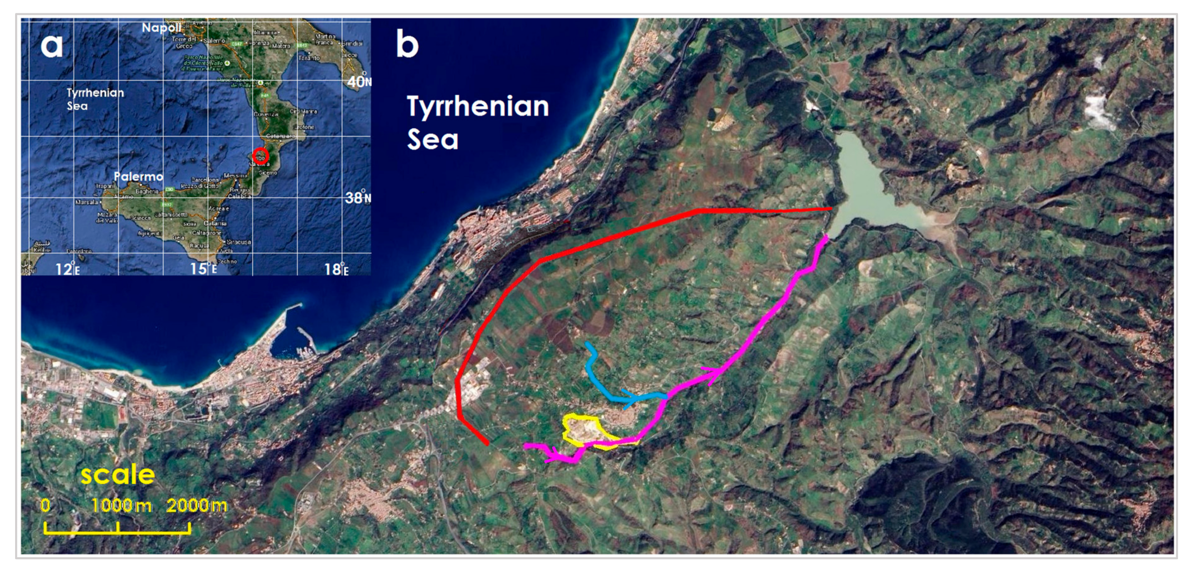
Figure 2.
Panoramic view and stratigraphic succession of the Maierato Landslide: the yellow line and the red line separate the strata.
Figure 2.
Panoramic view and stratigraphic succession of the Maierato Landslide: the yellow line and the red line separate the strata.

Figure 3.
The total station and the control panel (A). A target positioned on a building (B) and near the landslide crown (C).
Figure 3.
The total station and the control panel (A). A target positioned on a building (B) and near the landslide crown (C).

Figure 4.
Layout of the total station monitoring array, superimposed to the topographic map. The contour interval is 5 m. Yellow squares are points periodically surveyed by GNSS receivers, I1 and I2 are two boreholes which house inclinometers. The red line is the contour of the landslide. The dashed area is the main scarp. The pink line is the Scotrapiti ditch.

Figure 5.
Skyline from the monitoring total station.

Figure 6.
Cross sections of the landslide zone. The sections have been obtained along the directions connecting the total station S to the targets E1, E2, E4, E5, E7, and E9.
Figure 6.
Cross sections of the landslide zone. The sections have been obtained along the directions connecting the total station S to the targets E1, E2, E4, E5, E7, and E9.
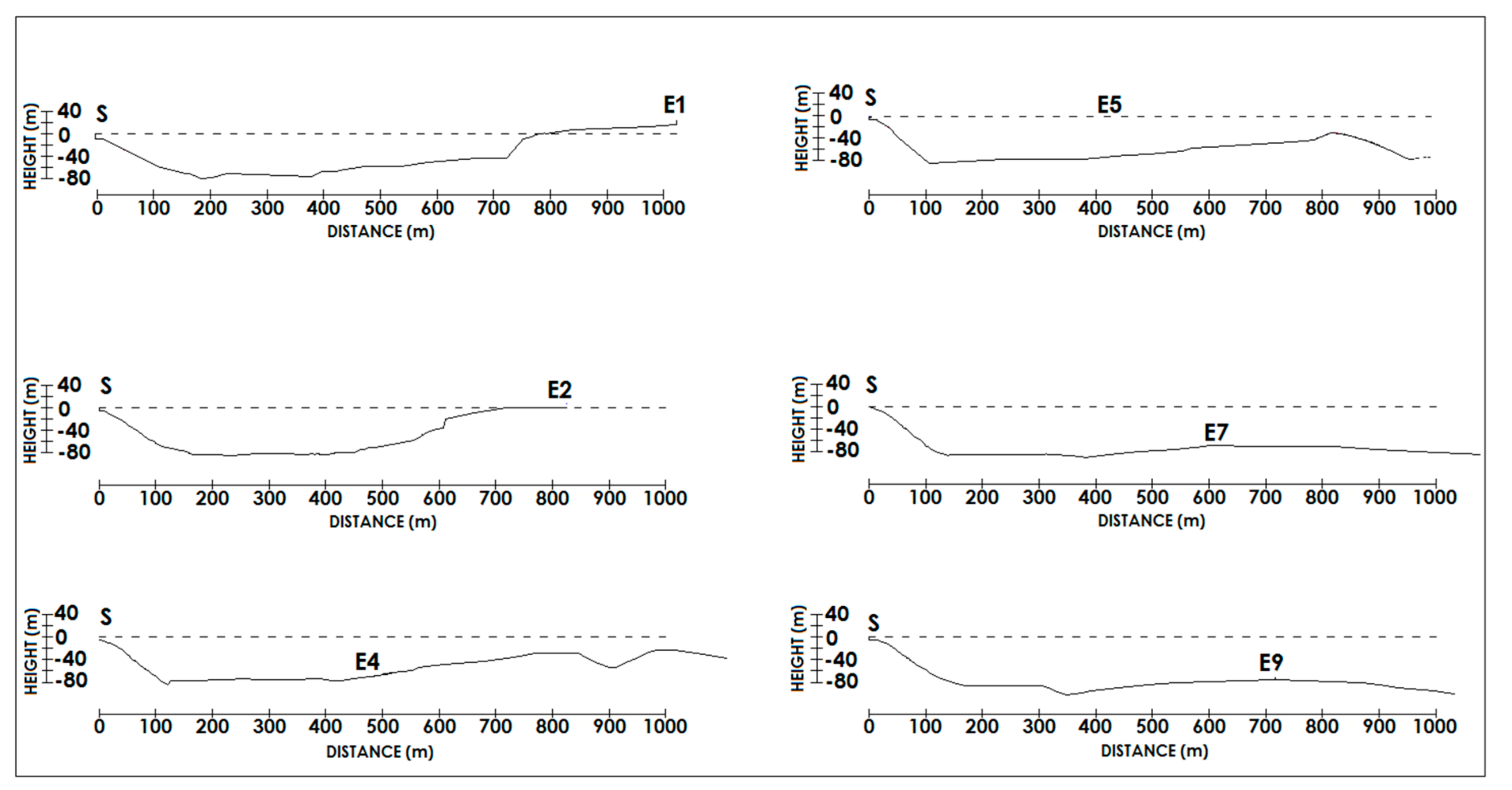
Figure 7.
(A) Slope distance Di for point E1 during the period June 2012 to September 2013: raw acquisition. (B) Slope distance Di for point E1 after applying Formula (1). Figure 7C is an enlargement of Figure 7A. (D) Slope distance Di for point E2 after applying Formula (1). The red lines represent the results after the application of a 300-point (four days) moving average filter.

Figure 8.
Slope distance Di for point E4 (a) and E9 (b) after applying the correction in ppm obtained by considering fixed the distance to E1.
Figure 8.
Slope distance Di for point E4 (a) and E9 (b) after applying the correction in ppm obtained by considering fixed the distance to E1.

Figure 9.
Slope distance for point E9 and daily temperature ranges in °C.
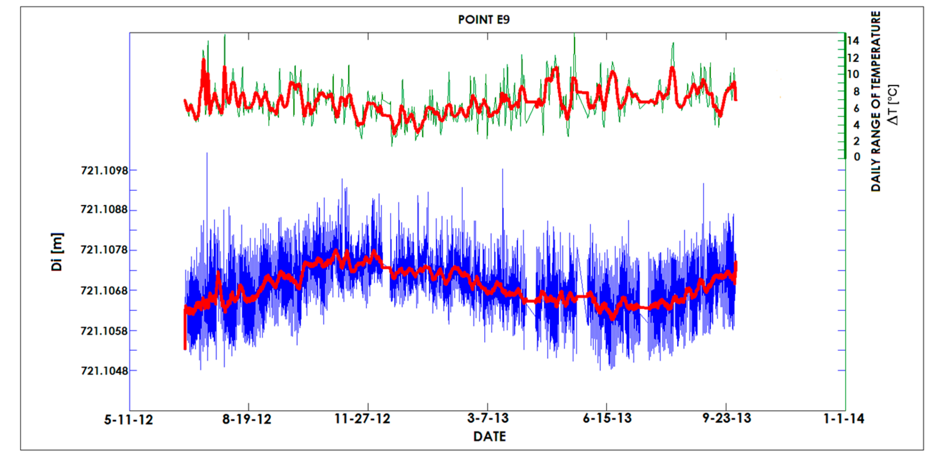
Figure 10.
Distances obtained, for a 10 days period, for targets E9 (A) and E4 (B) and temperatures measured by the weather station (C).
Figure 10.
Distances obtained, for a 10 days period, for targets E9 (A) and E4 (B) and temperatures measured by the weather station (C).

Figure 11.
Nearly linear relation between distance variations in ppm and daily temperature ranges ΔT for points E4, E5, E9, and regression lines. The black line is the regression line for the whole data set.
Figure 11.
Nearly linear relation between distance variations in ppm and daily temperature ranges ΔT for points E4, E5, E9, and regression lines. The black line is the regression line for the whole data set.
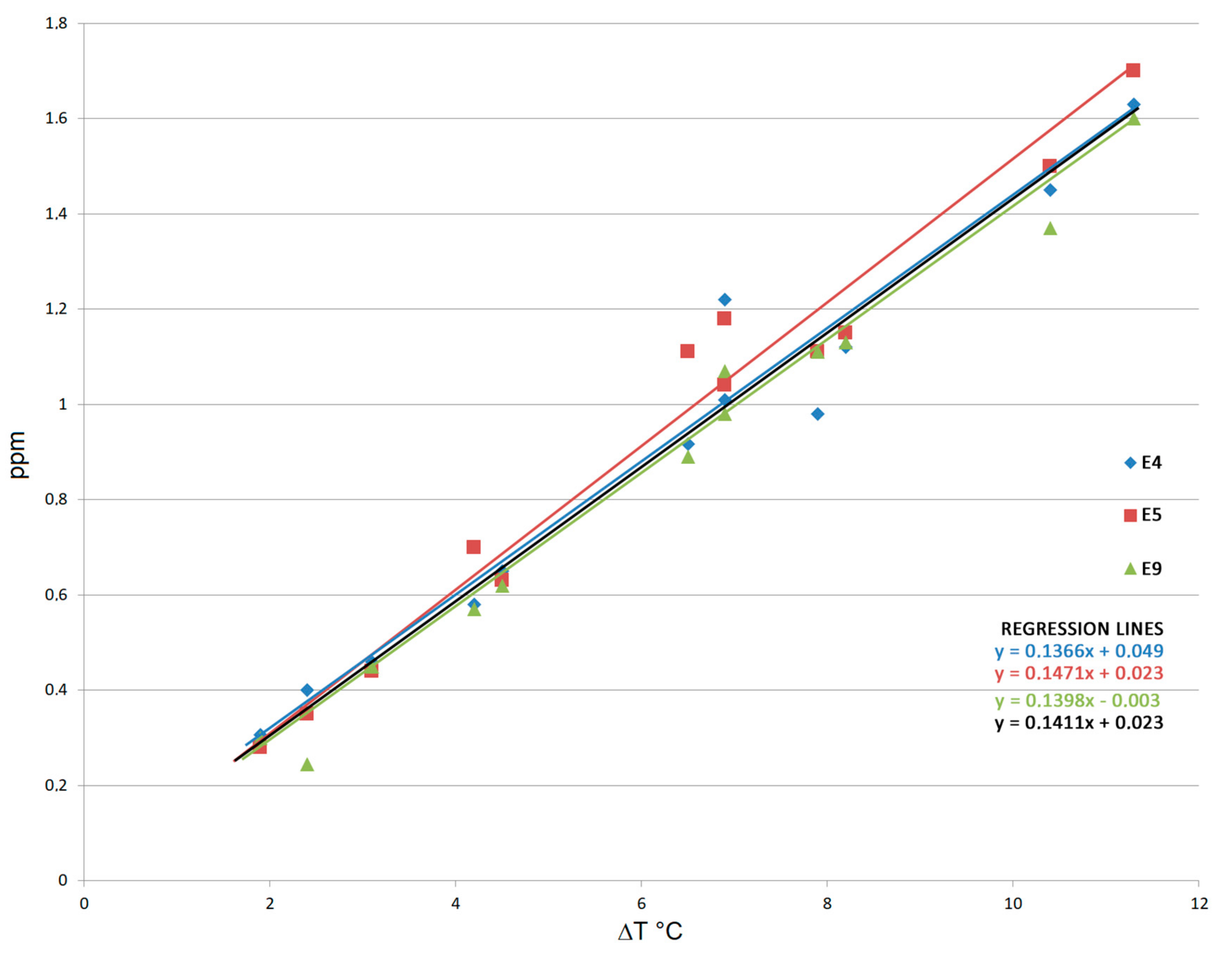
Figure 12.
Flow Chart.

Figure 13.
A perspective view of the DTM of the landslide superimposed to the aerial photo (the depleted zone is shown in beige, the filled one in green). Red lines are the laser paths from station S to the targets.
Figure 13.
A perspective view of the DTM of the landslide superimposed to the aerial photo (the depleted zone is shown in beige, the filled one in green). Red lines are the laser paths from station S to the targets.

Figure 14.
(A) From left to right: instantaneous solar lighting in the early morning, at noon and in the afternoon and map of average daily solar energy in MJ/m2day incident on the terrain, in the landslide zone, on 21 December. (B) Lighting and daily solar energy on 21 March. (C) Lighting and daily solar energy on 21 June. Black line is the contour of the landslide; red lines are the paths from the station to the targets.

Figure 15.
Variation of the difference between the temperatures of the air inside and outside the landslide zone (°C) for five sections, calculated for July. The sections have been obtained along the directions connecting the total station S to the targets.
Figure 15.
Variation of the difference between the temperatures of the air inside and outside the landslide zone (°C) for five sections, calculated for July. The sections have been obtained along the directions connecting the total station S to the targets.

Figure 16.
ppm corrections of the slope distances for the whole monitoring period, computed for target E4. (b) Enlargement of a 30 days period, circled in red in (a), along with the daily range of external air temperature.
Figure 16.
ppm corrections of the slope distances for the whole monitoring period, computed for target E4. (b) Enlargement of a 30 days period, circled in red in (a), along with the daily range of external air temperature.
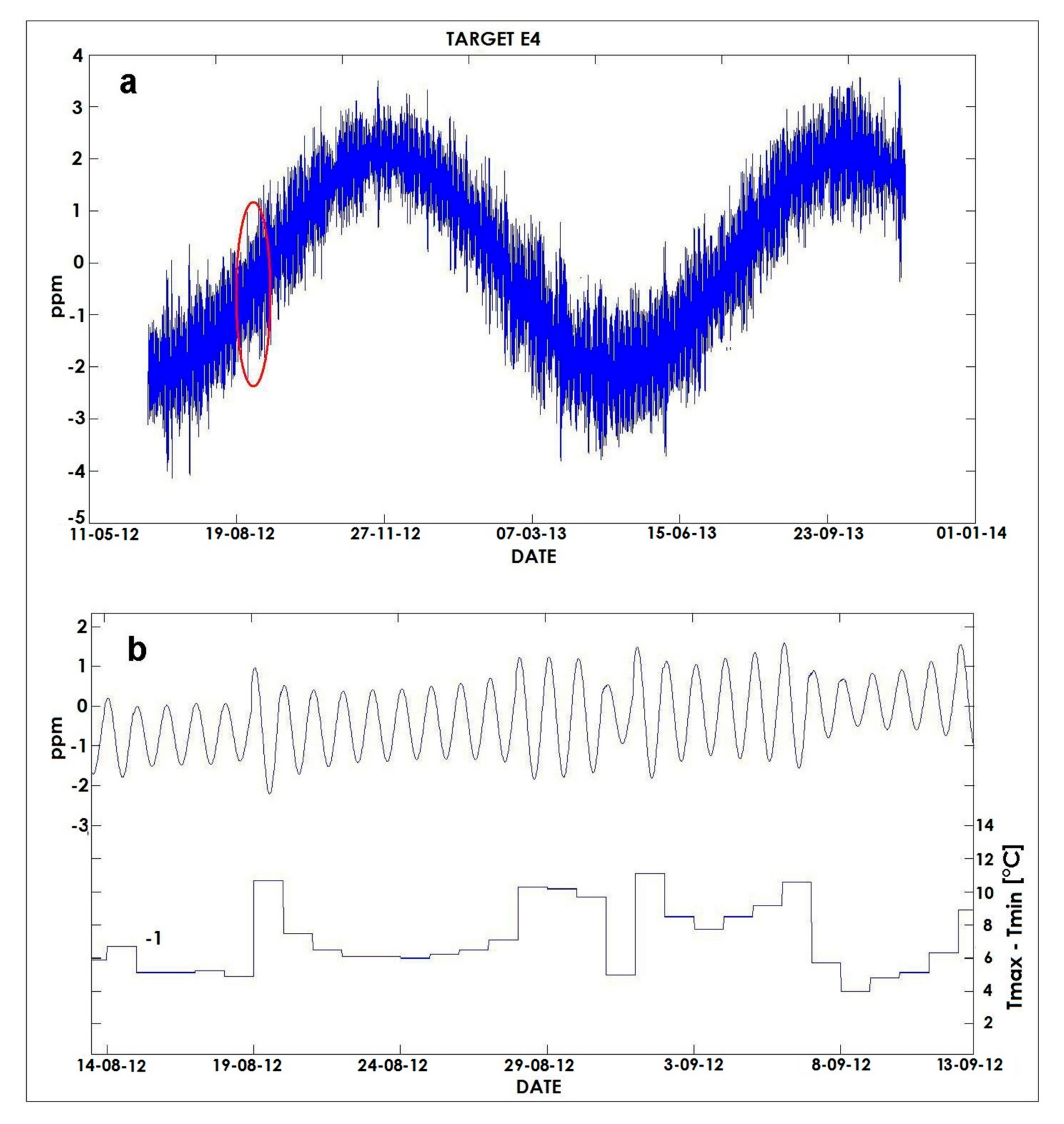
Figure 17.
Slope distances from the total station to the target E4, obtained by applying the ppm corrections computed by fixing the distance E1 (a) (Di ppm) and by using the methodology described in Section 2.6 (Di comp) (b).
Figure 17.
Slope distances from the total station to the target E4, obtained by applying the ppm corrections computed by fixing the distance E1 (a) (Di ppm) and by using the methodology described in Section 2.6 (Di comp) (b).

Figure 18.
Comparison between the distances of target E4, after applying only the daily correction (a) and once applied both daily and hourly correction (b).
Figure 18.
Comparison between the distances of target E4, after applying only the daily correction (a) and once applied both daily and hourly correction (b).

Table 1.
Main characteristics of the T30 total station.
| Angular Accuracy | 0.5″ |
|---|---|
| Pinpoint EDM accuracy | 0.6 mm + 1 ppm |
| Carrier wave | 658 nm |
| Automatic Target Recognition accuracy | 1″ |
| Measurement range without prism | 1000 m |
| Measurement range with a prism | 3500 m |
Table 2.
Atmospheric parameters for the Maierato area.
| Month | Solar Energy Hh (MJ/m2 day) | Diffuse/Global Solar Energy Ratio | Relative Humidity (%) | Wind Prevailing Direction | Wind Mean Speed (m/sec) | Minimum Tempera-ture (°C) | Maximum Tempera-ture (°C) | Mean Tempera-ture (°C) |
|---|---|---|---|---|---|---|---|---|
| 1 | 7.6 | 0.49 | 92 | SW - SE | 7.8 | 6.1 | 10.5 | 8.3 |
| 2 | 10.8 | 0.49 | 89 | SW - W | 8.2 | 5.6 | 10 | 7.8 |
| 3 | 14.7 | 0.44 | 81 | SW - W | 8.2 | 8.2 | 12.6 | 10.4 |
| 4 | 18.4 | 0.39 | 70 | W - SW | 7.9 | 10.6 | 15 | 12.8 |
| 5 | 22.2 | 0.39 | 58 | SW - W | 6.6 | 14.6 | 19 | 16.8 |
| 6 | 24.1 | 0.29 | 66 | SW- NW | 6.8 | 17.4 | 23.8 | 20.6 |
| 7 | 23.8 | 0.24 | 67 | NW- SW | 7.7 | 18.8 | 27.2 | 23 |
| 8 | 21 | 0.24 | 76 | NW- SW | 7.4 | 18.5 | 28.1 | 23.3 |
| 9 | 16.4 | 0.34 | 70 | NW- SW | 6.8 | 15.2 | 26.8 | 21 |
| 10 | 12.3 | 0.41 | 81 | SW - SE | 7.9 | 13.3 | 20.5 | 16.9 |
| 11 | 8.3 | 0.43 | 82 | SW - W | 8.7 | 11 | 15.4 | 13.2 |
| 12 | 6.7 | 0.48 | 83 | SW - SE | 8.4 | 7.5 | 11.5 | 9.5 |
| Year | 5678 | 0.35 | 76 | 7.7 | 13 | 18.9 | 15.8 |
Table 3.
Maximum corrections of slope distances (in ppm).
| Target | E4 | E5 | E6 | E7 | E8 | E9 |
|---|---|---|---|---|---|---|
| Aj | 2.10 | 1.90 | 1.25 | 0.77 | 0.70 | 0.65 |
Table 4.
Overall results of the measurements processing.
| Target | Di (m) | σraw (mm) | σtemp (mm) | σE1 (mm) | σtot (m) | σtot/σraw(%) | Declared EDM Accuracy (mm) |
|---|---|---|---|---|---|---|---|
| E4 | 490.7676 | 3.94 | 1.34 | 0.81 | 0.38 | 9.6 | 0.78 |
| E5 | 449.1439 | 2.74 | 1.26 | 0.62 | 0.30 | 10.9 | 0.75 |
| E6 | 622.5548 | 4.29 | 1.55 | 0.58 | 0.45 | 10.5 | 0.86 |
| E7 | 604.3088 | 4.37 | 1.47 | 0.48 | 0.40 | 9.2 | 0.85 |
| E8 | 649.9030 | 4.38 | 1.60 | 0.50 | 0.41 | 9.4 | 0.88 |
| E9 | 721.1069 | 5.13 | 1.71 | 0.65 | 0.45 | 8.8 | 0.94 |
© 2018 by the authors. Licensee MDPI, Basel, Switzerland. This article is an open access article distributed under the terms and conditions of the Creative Commons Attribution (CC BY) license (http://creativecommons.org/licenses/by/4.0/).
Share and Cite
MDPI and ACS Style
Artese, S.; Perrelli, M. Monitoring a Landslide with High Accuracy by Total Station: A DTM-Based Model to Correct for the Atmospheric Effects. Geosciences 2018, 8, 46. https://doi.org/10.3390/geosciences8020046
AMA Style
Artese S, Perrelli M. Monitoring a Landslide with High Accuracy by Total Station: A DTM-Based Model to Correct for the Atmospheric Effects. Geosciences. 2018; 8(2):46. https://doi.org/10.3390/geosciences8020046
Chicago/Turabian StyleArtese, Serena, and Michele Perrelli. 2018. "Monitoring a Landslide with High Accuracy by Total Station: A DTM-Based Model to Correct for the Atmospheric Effects" Geosciences 8, no. 2: 46. https://doi.org/10.3390/geosciences8020046
Note that from the first issue of 2016, this journal uses article numbers instead of page numbers. See further details here.