Recognizing Vertical and Lateral Variability in Terrestrial Landscapes: A Case Study from the Paleosols of the Late Pennsylvanian Casselman Formation (Conemaugh Group) Southeast Ohio, USA

Abstract
:1. Introduction
2. Geologic Setting
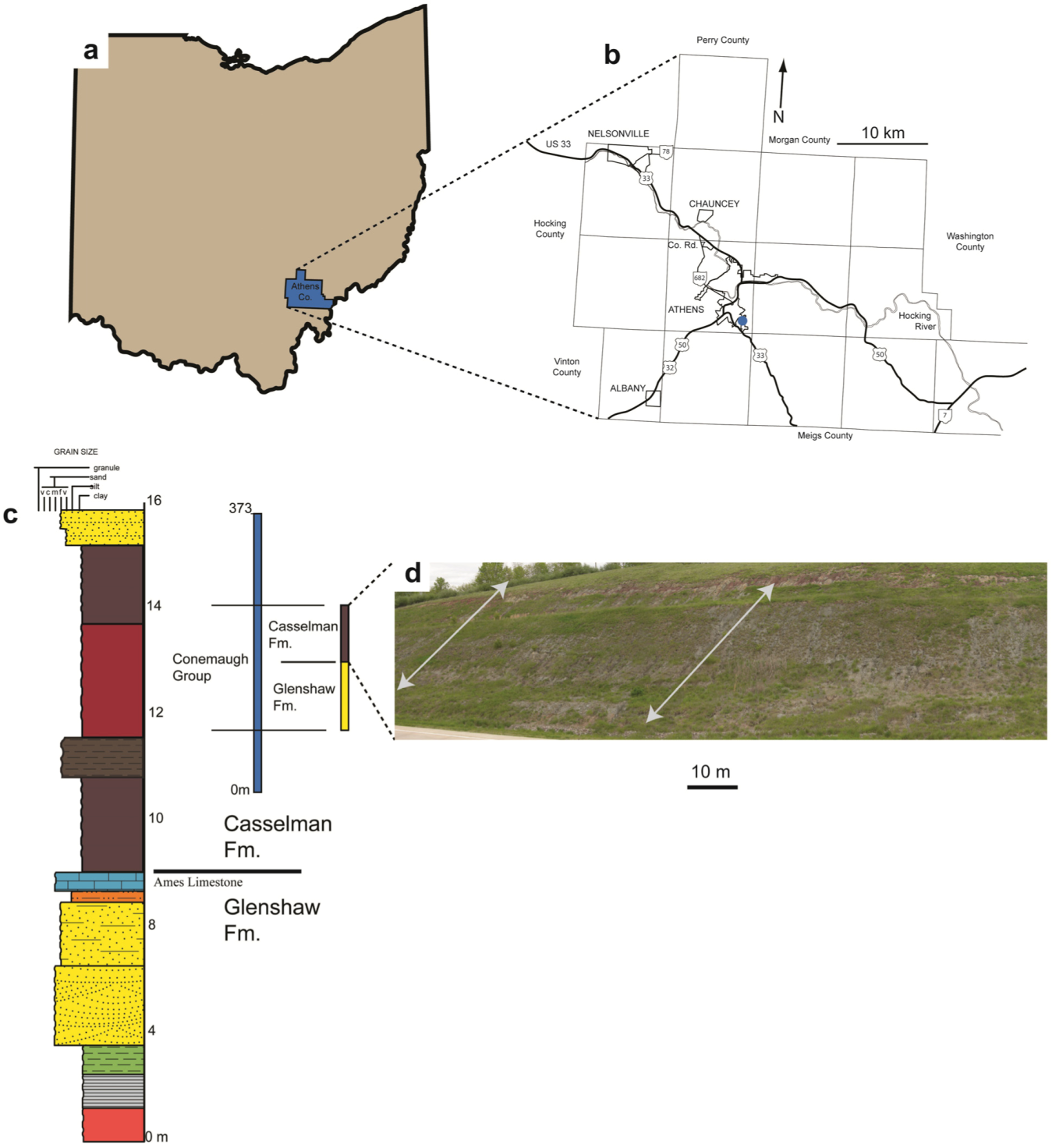
3. Methods
4. Results
4.1. Continental Ichnology of the Casselman Formation


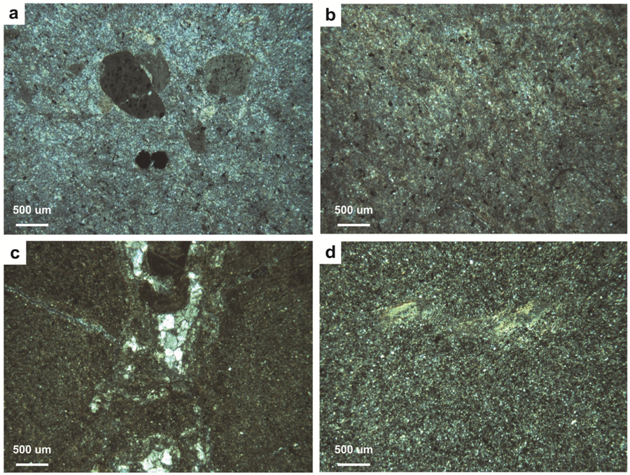
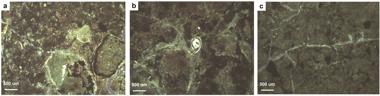
4.2. Paleopedology of the Casselman Formation
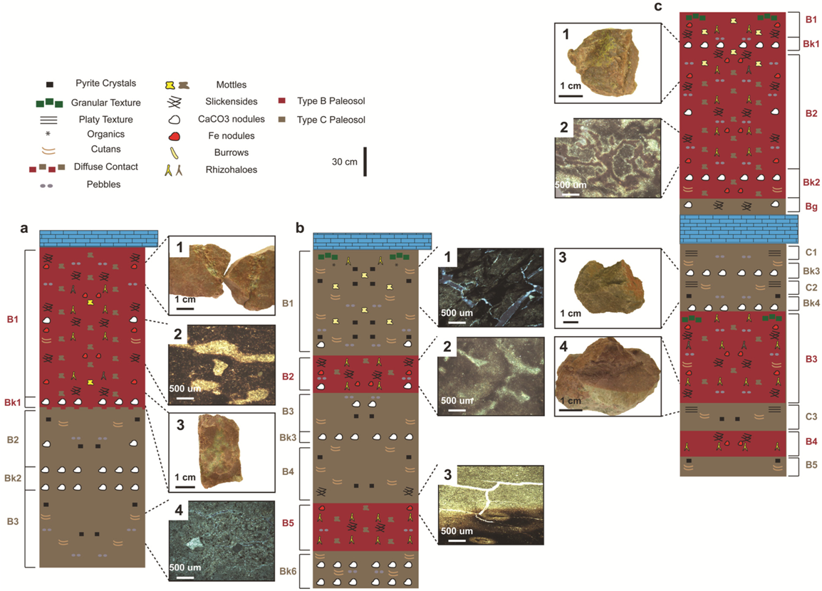
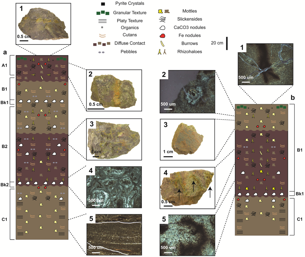
4.2.1. Type A Paleosols

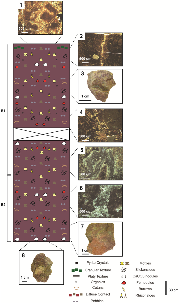
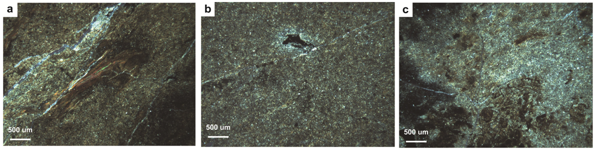
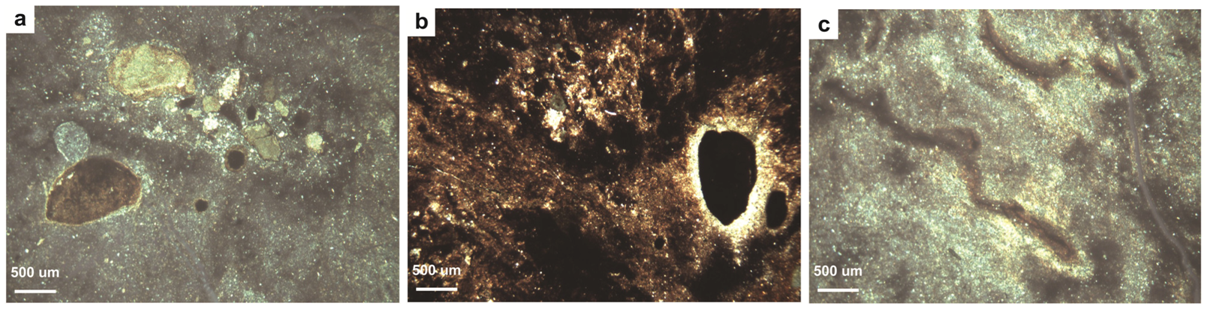
4.2.2. Type B Paleosols

4.2.3. Type C Paleosols

4.2.4. Type D Paleosols

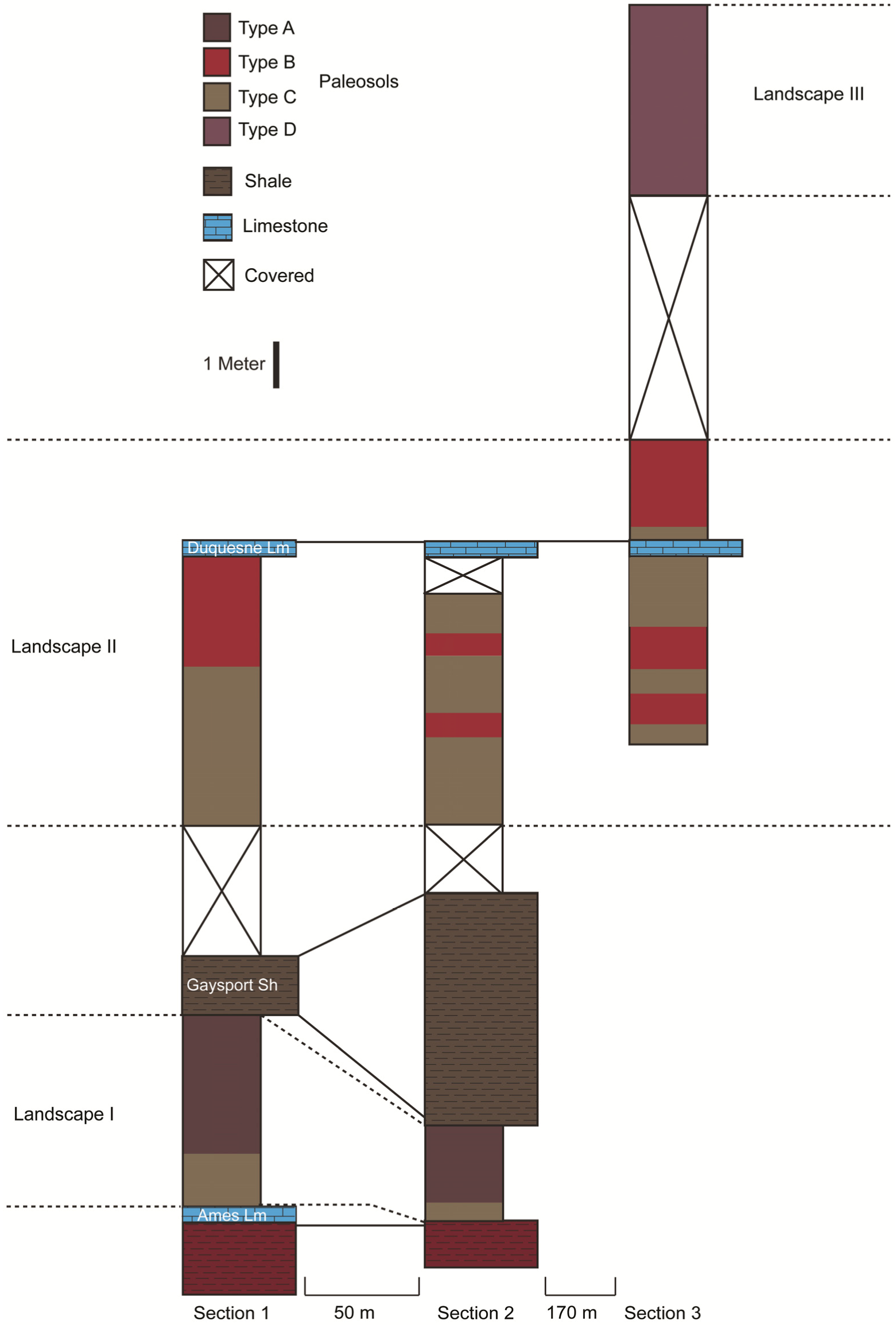
5. Discussion
5.1. Casselman Landscapes
5.2. Variability within the Paleosols of the Casselman Formation
6. Conclusions
Acknowledgments
References
- Frey, R.W. The Lebensspuren of some common marine invertebrates near Beaufort, North Carolina. II. Anemone burrows. J. Paleontol. 1970, 44, 308–311. [Google Scholar]
- Rhoads, D.C. The paleoecological and environmental significance of trace fossils. In The Study of Trace Fossils; Frey, R.W., Ed.; Springer-Verlag: New York, NY, USA, 1975. [Google Scholar]
- Seilacher, A.; Seilacher, E. Bivalvian trace fossils: A lesson from actuopaleontology. Cour. Forschungsinst. Senckenb. 1994, 169, 5–15. [Google Scholar]
- Bromley, R.G. Trace Fossils: Biology, Taphonomy and Applications, 2nd ed; Chapman & Hall: London, UK, 1996. [Google Scholar]
- Uchman, A.; Pervesler, P. Surface lebensspuren produced by amphipods and isopods (crustaceans) from the Isonzo delta tidal flat, Italy. Palaios 2006, 21, 384–390. [Google Scholar] [CrossRef]
- Gingras, M.; Bann, K.; MacEachern, J.; Pemberton, S. A conceptual framework for the application of trace fossils. In Applied Ichnolgy; MacEachern, J.A., Bann, K.L., Gingras, M.K., Pemberton, S.G., Eds.; SEPM Short Course Notes 52; Society for Sedimentary Geology: Tulsa, OK, USA, 2007; pp. 1–25. [Google Scholar]
- Joeckel, R. Paleosols below the Ames Marine Unit (Upper Pennsylvanian, Conemaugh Group) in the Appalachian Basin, USA; Variability on an ancient depositional landscape. J. Sediment. Res. 1995, 65, 393–407. [Google Scholar]
- Kraus, M.J. Paleosols in clastic sedimentary rocks: Their geologic applications. Earth Sci. Rev. 1999, 47, 41–70. [Google Scholar] [CrossRef]
- Retallack, G.J. Late Oligocene bunch grassland and early Miocene sod grassland paleosols from central Oregon, USA. Palaeogeogr. Palaeoclimatol. Palaeoecol. 2004, 207, 203–237. [Google Scholar] [CrossRef]
- Driese, S.G.; Ober, E.G. Paleopedologic and paleohydrologic records of precipitation seasonality from Early Pennsylvanian “underclay” paleosols, USA. J. Sediment. Res. 2005, 75, 997–1010. [Google Scholar] [CrossRef]
- Kraus, M.J.; Hasiotis, S.T. Significance of different modes of rhizolith preservation to interpreting paleoenvironmental and paleohydrologic settings: Examples from Paleogene paleosols, Bighorn Basin, Wyoming, USA. J. Sediment. Res. 2006, 76, 633–646. [Google Scholar] [CrossRef]
- Hembree, D.I.; Hasiotis, S.T. Paleosols and ichnofossils of the White River Formation of Colorado: Insight into soil ecosystems of the North American Midcontinent during the Eocene-Oligocene transition. Palaios 2007, 22, 123–142. [Google Scholar] [CrossRef]
- Hembree, D.I.; Nadon, G.C. A paleopedologic and ichnologic perspective of the terrestrial Pennsylvanian landscape in the distal Appalachian Basin, USA. Palaeogeogr. Palaeoclimatol. Palaeoecol. 2011, 312, 138–166. [Google Scholar] [CrossRef]
- Kraus, M.J.; Bown, T.M. Paleosols and time resolution in alluvial stratigraphy. In Paleosols: Their Recognition and Interpretation; Wright, V.P., Ed.; Princeton University Press: Princeton, NJ, USA, 1986; pp. 180–207. [Google Scholar]
- Retallack, G.J.; Mindszenty, A. Well preserved late Precambrian paleosols from northwest Scotland. J. Sediment. Res. 1994, 64, 264–281. [Google Scholar]
- Smith, J.J.; Hasiotis, S.T.; Kraus, M.J.; Woody, D.T. Relationship of floodplain ichnocoenoses to paleopedology, paleohydrology, and paleoclimate in the Willwood Formation, Wyoming, during the Paleocene–Eocene Thermal Maximum. Palaios 2008, 23, 683–699. [Google Scholar] [CrossRef]
- Tabor, N.J.; Montañez, I.P.; Scotese, C.R.; Poulsen, C.J.; Mack, G.H. Paleosol archives of environmental and climatic history in paleotropical western Pangea during the latest Pennsylvanian through Early Permian. In Resolving the Late Paleozoic Ice Age in Time and Space; Frank, T.D., Isbell, J.L., Eds.; Geological Society of America: Boulder, CO, USA, 2008; pp. 291–304. [Google Scholar]
- Sheldon, N.D.; Tabor, N.J. Quantitative paleoenvironmental and paleoclimatic reconstruction using paleosols. Earth Sci. Rev. 2009, 95, 1–52. [Google Scholar] [CrossRef]
- Aslan, A.; Autin, W.J. Holocene flood-plain soil formation in the southern lower Mississippi Valley: Implications for interpreting alluvial paleosols. Geol. Soc. Am. Bull. 1998, 110, 433–449. [Google Scholar]
- Retallack, G.J. Soils of the Past: An Introduction to Paleopedology, 2nd ed; Blackwell Science Ltd.: Oxford, UK, 2001. [Google Scholar]
- Buol, S.W. Soil Genesis and Classification, 5th ed; Blackwell Publishing: Ames, IA, USA, 2003. [Google Scholar]
- Schaetzl, R.J.; Anderson, S. Soils: Genesis and Geomorphology; Cambridge University Press: Cambridge, UK, 2009. [Google Scholar]
- Hembree, D.I.; Hasiotis, S.T. Miocene vertebrate and invertebrate burrows defining compound paleosols in the Pawnee Creek Formation, Colorado, USA. Palaeogeogr. Palaeoclimatol. Palaeoecol. 2008, 270, 349–365. [Google Scholar] [CrossRef]
- Retallack, G.J.; Amundson, R.; Harden, J.; Singer, M. The environmental factor approach to the interpretation of paleosols. In Factors of Soil Formation: A Fiftieth Anniversary Retrospective, Special Publication of the Soil Science Society of America 33; Amundson, R., Harden, J., Singer, M., Eds.; Soil Science Society of America: Madison, WI, USA, 1994; pp. 31–64. [Google Scholar]
- Retallack, G.J. Pedogenic carbonate proxies for amount and seasonality of precipitation in paleosols. Geology 2005, 33, 333–336. [Google Scholar] [CrossRef]
- Tabor, N.J.; Montañez, I.P.; Kelso, K.A.; Currie, B.; Shipman, T.; Colombi, C.A. Late Triassic soil catena: Landscape and climate controls on paleosol morphology and chemistry across the Carnian-age Ischigualasto-Villa Union Basin, northwestern Argentina. Spec. Pap. Geol. Soc. Am. 2006, 416, 17–41. [Google Scholar]
- Hasiotis, S.T. Complex ichnofossils of solitary and social soil organisms: Understanding their evolution and roles in terrestrial paleoecosystems. Palaeogeogr. Palaeoclimatol. Palaeoecol. 2003, 192, 259–320. [Google Scholar] [CrossRef]
- Hasiotis, S.T. Reconnaissance of Upper Jurassic Morrison Formation ichnofossils, Rocky Mountain Region, USA: Paleoenvironmental, stratigraphic, and paleoclimatic significance of terrestrial and freshwater ichnocoenoses. Sediment. Geol. 2004, 167, 177–268. [Google Scholar] [CrossRef]
- Kraus, M.J.; Riggins, S. Transient drying during the Paleocene-Eocene thermal maximum (PETM): Analysis of paleosols in the Bighorn Basin, Wyoming. Palaeogeog. Palaeoclimatol. Palaeoecol. 2007, 245, 444–461. [Google Scholar] [CrossRef]
- Therrien, F.; Zelenitsky, D.K.; Weishampel, D.B. Palaeoenvironmental reconstruction of the Late Cretaceous Sânpetru Formation (Hateg Basin, Romania) using paleosols and implications for the “disappearance” of dinosaurs. Palaeogeogr. Palaeoclimatol. Palaeoecol. 2009, 272, 37–52. [Google Scholar] [CrossRef]
- Hembree, D.I.; Martin, L.D.; Hasiotis, S.T. Amphibian burrows and ephemeral ponds of the Lower Permian Speiser Shale, Kansas: Evidence for seasonality in the midcontinent. Palaeogeogr. Palaeoclimatol. Palaeoecol. 2004, 203, 127–152. [Google Scholar] [CrossRef]
- Smith, J.J.; Hasiotis, S.T. Traces and burrowing behaviors of the cicada nymph Cicadetta calliope: Neoichnology and paleoecological significance of extant soil-dwelling insects. Palaios 2008, 23, 503–513. [Google Scholar] [CrossRef]
- Melchor, R.N.; Genise, J.F.; Farina, J.L.; Sánchez, M.V.; Sarzetti, L.; Visconti, G. Large striated burrows from fluvial deposits of the Neogene Vinchina Formation, La Rioja, Argentina: A crab origin suggested by neoichnology and sedimentology. Palaeogeogr. Palaeoclimatol. Palaeoecol. 2010, 291, 400–418. [Google Scholar] [CrossRef]
- Sturgeon, M.T. The Geology and Mineral Resources of Athens County, Ohio; State of Ohio Division of Geological Survey: Columbus, OH, USA, 1958. [Google Scholar]
- McDowell, R. An interpretation of the Grafton sandstone and its implications for Pennsylvanian paleohydraulics, climate, provenance, and tectonics. Compass Sigma Gamma Epsil. 1986, 63, 48–57. [Google Scholar]
- Milici, R.C.; Swezey, C.S. Assessment of Appalachian Basin Oil and Gas Resources: Devonian Shale—Middle and Upper Paleozoic Total Petroleum System; U.S. Geological Survey Open-File Report 2006-1237; U.S. Geological Survey: Reston, VA, USA, 2006.
- Chesnut, D.R., Jr. Timing of the Alleghenian tectonics determined by Central Appalachian foreland basin analysis. Southeast. Geol. 1991, 31, 203–221. [Google Scholar]
- Edmunds, W.E.; Skema, V.W.; Flint, N.K. Pennsylvanian. In The Geology of Pennsylvania—SpecialPublication 1; Pennsylvania Geological Survey: Middletown; Pittsburgh Geological Society: Pittsburgh, PA, USA, 1999. [Google Scholar]
- Belt, E.S.; Heckel, P.H.; Lentz, L.J.; Bragonier, W.A.; Lyons, T.W. Record of glacial-eustatic sea-level fluctuations in complex middle to late Pennsylvanian facies in the Northern Appalachian Basin and relation to similar events in the Midcontinent basin. Sediment. Geol. 2011, 238, 79–100. [Google Scholar] [CrossRef]
- Donaldson, A.; Renton, J.; Presley, M. Pennsylvanian deposystems and paleoclimates of the Appalachians. Int. J. Coal Geol. 1985, 5, 167–193. [Google Scholar] [CrossRef]
- Opdyke, N.; DiVenere, V. Paleomagnetism and Carboniferous climate. In Predictive Stratigraphic Analysis: Concept and Application; Cecil, C.B., Edgar, N.T., Eds.; U.S. Geological Survey Bulletin 2110; U.S. Government Printing Office: Washington, DC, USA, 1994; pp. 8–9. [Google Scholar]
- Brezinski, D. Developmental model for an Appalachian Pennsylvanian marine incursion. Northeast. Geol. 1983, 5, 92–95. [Google Scholar]
- Scotese, C.R. Carboniferous paleocontinental reconstructions. In Predictive Stratigraphic Analysis: Concept and Application; Cecil, C.B., Edgar, N.T., Eds.; U.S. Geological Survey Bulletin 2110; U.S. Government Printing Office: Washington, DC, USA, 1994; pp. 3–5. [Google Scholar]
- Heckel, P.H. Glacial-eustatic base-level-climatic model for late Middle to Late Pennsylvanian coal-bed formation in the Appalachian Basin. J. Sediment. Res. 1995, 65, 348–356. [Google Scholar]
- Nadon, G.; Kelly, R. The constraints of glacial eustasy and low accommodation on sequence stratigraphic interpretations of Pennsylvanian strata, Conemaugh Group, Appalachian basin, USA. In Sequence Stratigraphy, Paleoclimate, and Tectonics of Coal-Bearing Strata; Pashin, J.C., Gastaldo, R.A., Eds.; AAPG: Tulsa, OK, USA, 2004; pp. 29–44. [Google Scholar]
- Rygel, M.C.; Fielding, C.R.; Frank, T.D.; Birgenheier, L.P. The magnitude of late Paleozoic glacioeustatic fluctuations: A synthesis. J. Sediment. Res. 2008, 78, 500–511. [Google Scholar] [CrossRef]
- Heckel, P.H. Pennsylvanian cyclothems in Midcontinent North America as far-field effects of waxing and waning of Gondwana ice sheets. In Resolving the Late Paleozoic Ice Age in Time and Space; Fielding, C.R., Frank, T.D., Isbell, J.L., Eds.; Geological Society of America: Boulder, CO, USA, 2008; pp. 275–290. [Google Scholar]
- Merrill, G. Lithostratigraphy and lithogenesis of Conemaugh (Carboniferous) depositional systems near Huntington, West Virginia. Southeast. Geol. 1986, 28, 155–171. [Google Scholar]
- Lebold, J.G.; Kammer, T.W. Gradient analysis of faunal distributions associated with rapid transgression and low accommodation space in a Late Pennsylvanian marine embayment: Biofacies of the Ames Member (Glenshaw Formation, Conemaugh Group) in the northern Appalachian Basin, USA. Palaeogeogr. Palaeoclimatol. Palaeoecol. 2006, 231, 291–314. [Google Scholar] [CrossRef]
- Cormany, C.R. The Fluvial Architecture of the Upper Casselman Formation, Conemaugh Group (Pennsylvanian), Athens County, Ohio. Master’s Thesis, Ohio University, Athens, OH, USA, 2001. [Google Scholar]
- Tabor, N.J.; Montanez, I.P. Morphology and distribution of fossil soils in the Permo-Pennsylvanian Wichita and Bowie Groups, north-central Texas, USA: Implications for western equatorial Pangean palaeoclimate during icehouse-greenhouse transition. Sedimentology 2004, 51, 851–884. [Google Scholar] [CrossRef]
- Cecil, C.B.; Dulong, F.T.; West, R.R.; Stamm, R.; Wardlaw, B.; Edgar, N.T. Climate controls on the stratigraphy of a Middle Pennsylvanian cyclothem in North America. SEPM Spec. Publ. 2003, 77, 151–182. [Google Scholar]
- Falcon-Lang, H.J.; Heckel, P.H.; Dimichele, W.A.; Bascomb, M.; Blake, J.; Easterday, C.R.; Eble, C.F.; Elrick, S.; Gastaldo, R.A.; Greb, S.F.; Martino, R.L. No major stratigraphic gap exists near the Middle–Upper Pennsylvanian (Desmoinesian–Missourian) boundary in North America. Palaios 2011, 26, 125–139. [Google Scholar] [CrossRef]
- Brewer, R. Fabric and Mineral Analysis of Soils, 2nd ed; Krieger: New York, NY, USA, 1976. [Google Scholar]
- Fitzpatrick, E.A. Soil Microscopy and Micromorphology; John Wiley & Sons: New York, NY, USA, 1993. [Google Scholar]
- Mack, G.H.; James, W.C.; Monger, H.C. Classification of paleosols. Geol. Soc. Am. Bull. 1993, 105, 129–136. [Google Scholar]
- NRCS Soils, Keys to Soil Taxonomy, 11th ed; USDA Natural Resources Conservation Service: Washington, DC, USA, 2010.
- Bertling, M.; Braddy, S.J.; Bromley, R.G.; Demathieu, G.R.; Genise, J.; Mikul, R.; Nielsen, J. K.; Nielsen, K. S.S.; Rindsberg, A.K.; Schlirf, M. Names for trace fossils: A uniform approach. Lethaia 2006, 39, 265–286. [Google Scholar] [CrossRef]
- D’Alessandro, A.; Bromley, R.G. Meniscate trace fossils and the Muensteria-Taenidium problem. Palaeontology 1987, 30, 743–763. [Google Scholar]
- Hasiotis, S.T.; van Wagoner, J.C. Continental Trace Fossils; SEPM Short Course Notes 51; SEPM Society for Sedimentary: Tulsa, OK, USA, 2002. [Google Scholar]
- Gingras, M.K.; Pemberton, S.G.; Mendoza, C.; Henk, F.H. Modeling fluid flow in trace fossils: Assessing the anisotropic permeability of Glossifungites surfaces. Petrol. Geosci. 1999, 5, 349–357. [Google Scholar] [CrossRef]
- Hasiotis, S.; Kraus, M.; Demko, T. Climate controls on continental trace fossils. In Trace Fossils: Concepts, Problems, Prospects; Miller, W., III, Ed.; Elsevier: Amsterdam, The Netherlands, 2007; pp. 172–195. [Google Scholar]
- Mason, J.A; Jacobs, P.M. Nature of Quaternary paleosols. In Encyclopedia of Quaternary Science; Elias, S., Ed.; Elsevier: Amsterdam, The Netherlands, 2007. [Google Scholar]
- LePage, B.; Pfefferkorn, H. Did ground cover change over geologic time? Paleontol. Soc. Pap. 2000, 6, 171–182. [Google Scholar]
- DiMichele, W.A.; Pfefferkorn, H.W.; Gastaldo, R.A. Response of Late Carboniferous and Early Permian plant communities to climate change. Annu. Rev. Earth Planet. Sci. 2001, 29, 461–487. [Google Scholar] [CrossRef]
- Stiles, C.A.; Mora, C.I.; Driese, S.G. Pedogenic iron-manganese nodules in Vertisols: A new proxy for paleoprecipitation? Geology 2001, 29, 943. [Google Scholar] [CrossRef]
- Thomas, B.A. Paleozoic Herbaceous Lycopsids and the beginnings of extant Lycopodium Sens Lat. and Selaginella Sens. Lat. Ann. Mo. Bot. Gard. 1992, 79, 623–631. [Google Scholar] [CrossRef]
- Collinson, J. Alluvial sediments. In Sedimentary Environments: Processes, Facies and Stratigraphy, 3rd; Reading, H.G., Ed.; Blackwell Sciences Ltd.: Oxford, UK, 1996; pp. 37–82. [Google Scholar]
© 2012 by the authors; licensee MDPI, Basel, Switzerland. This article is an open-access article distributed under the terms and conditions of the Creative Commons Attribution license (http://creativecommons.org/licenses/by/3.0/).
Share and Cite
Catena, A.; Hembree, D. Recognizing Vertical and Lateral Variability in Terrestrial Landscapes: A Case Study from the Paleosols of the Late Pennsylvanian Casselman Formation (Conemaugh Group) Southeast Ohio, USA. Geosciences 2012, 2, 178-202. https://doi.org/10.3390/geosciences2040178
Catena A, Hembree D. Recognizing Vertical and Lateral Variability in Terrestrial Landscapes: A Case Study from the Paleosols of the Late Pennsylvanian Casselman Formation (Conemaugh Group) Southeast Ohio, USA. Geosciences. 2012; 2(4):178-202. https://doi.org/10.3390/geosciences2040178
Chicago/Turabian StyleCatena, Angeline, and Daniel Hembree. 2012. "Recognizing Vertical and Lateral Variability in Terrestrial Landscapes: A Case Study from the Paleosols of the Late Pennsylvanian Casselman Formation (Conemaugh Group) Southeast Ohio, USA" Geosciences 2, no. 4: 178-202. https://doi.org/10.3390/geosciences2040178