
Development of a Hydraulic Actuator for MRI- and Radiation-Compatible Medical Applications

Mechatronics Group, Technische Universität Ilmenau, 98693 Ilmenau, Germany
*
Author to whom correspondence should be addressed.
Actuators 2024, 13(3), 90; https://doi.org/10.3390/act13030090
Submission received: 25 January 2024
/
Revised: 9 February 2024
/
Accepted: 18 February 2024
/
Published: 27 February 2024
(This article belongs to the Section Actuators for Medical Instruments)
Abstract
:This paper presents methods for the actuation, measurement, and control of a magnetic resonance imaging- and radiation-compatible single-axis translatory actuation system. As an exemplary demanding use case, the axis is developed for a robotic phantom for evaluating emitted radiation doses of radiotherapy devices. For this, the robot has to follow given three-dimensional trajectories of patients’ movements with an accuracy of 200 µm. For enabling use of magnetic resonance imaging, actuation of the robot is realized by hydraulic transmission without any metal parts or electrical components at the imaging side. The hydraulic axis is developed, built-up, and tested. In order to compensate for deviations from the targeted actuation trajectory resulting from tolerances, friction, and non-linearities in the system, a combination of photogrammetric measurement and iterative learning control is applied. The developed photogrammetric system is capable of determining the robot’s position with systematic errors of 35 µm and stochastic errors of 0.3 µm. Different types of iterative learning control methods are applied, parameterized, and tested. With this, the hydraulically actuated axis is able to follow given trajectories with maximum errors below 130 µm.
1. Introduction
Many different diseases and injuries of the human body, such as fractures, tumors, neurological dysfunctions, rheumatism, etc., require surgical diagnostics and interventions. For this, many medical imaging as well as intervention devices are necessary, on which high demands regarding quality assurance, compatibility, and safety are placed. In the field of surgery, a growing trend towards medical robots can be observed with the overall promise of shortening surgical procedures, increasing the accuracy and repeatability of movements, and, hence, increasing patient safety with reduced procedure costs [1,2,3]. While these robotic systems exhibit many different working principles, a common problem for all of them is precise and robust actuation, while not being influenced by or influencing other surrounding medical devices.
1.1. Demands on Actuation Systems in Medical Environments
In particular, the latter demand leads to the question of compatibility with medical imaging devices. Magnetic resonance imaging (MRI) devices exhibit strong magnetic fields, which also include alternating fields. In metal parts, this leads to eddy currents, resulting in heat dissipation. Furthermore, artifacts in the imaging process can deteriorate the medical image depending on the specifically used conducting materials [4]. Another effect is forces acting on the component. This is why metal parts are usually forbidden in the vicinity of MRI devices [5].
Another commonly used medical imaging tool is the computed tomography (CT) scanner and other types of X-ray-based devices. They are also prone to imaging artifacts resulting from the use of specific materials and their X-ray dispersion [6,7]. Additionally, the radiation itself is known to damage electrical components, especially microelectronics. This may not destroy the actuation system on the first run; however, the damage to the individual components will accumulate with the growing number of deployment of the actuation system in such environments, eventually leading to a failure in functionality. Also, the emitted radiation from radiotherapy devices has similar effects on medical actuation systems, with usually much higher doses of ionizing radiation [8].
Other common demands on medical devices are typically electromagnetic compatibility, sterilizability, and the need for ease of handling by medical personnel. For the actuation itself, depending on the specific use case, a combination of high precision, high dynamics, and/or high static forces is desired. In summary, this leads to the question of feasible actuation principles when working under environments with both MRI and radiation sources. Both MR-compatibility and positioning accuracy is already addressed in other MR-compatible robotic systems, applied, for example, for prostate, neurosurgical, breast cancer, or other surgical interventions, as outlined in [9]. Therein, the positioning accuracy for different actuation principles are compared; however, the relationships between workspace, stroke, and force are not considered. Many actuation approaches for MRI application use piezoelectric or pneumatic actuation and achieve positioning accuracy in the mm-range, and for a few prototypes, in the sub-mm range.
This paper provides a contribution through the development of a single-axis actuation system compatible for use in medical environments in the presence of MRI and radiation. In order to illustrate the development process and the occurring problems, the development is performed for the highly demanding specific use case of a radiotherapy robotic phantom, which is described in the following section.
1.2. Robotic Phantoms for Radiotherapy
Radiotherapy is a method to treat malignant tumors. It uses ionizing radiation to destroy tumor cells in various parts of the human body. Unavoidable periodic patient movements, e.g., breathing, heartbeats, or peristalsis of the digestive tract, are overcome by tracking these movements and adapting the radiation source to it in order to leave non-tumor tissue unharmed during patient movements [8]. The tracking is usually performed by simultaneous deployment of MRI. For validating radiotherapy devices and their beam focus adaption mechanism, so-called robotic phantoms simulate the specific movements and radiation absorption of a human body, while measuring the emitted radiation dose on these tissue parts [10,11]. A prototype of this robot is depicted in Figure 1.
The paper [11] surveys the state of the art of parallel manipulators for phantom robotic platforms. There, it is stated that the current prototypes and products are either complex and error-prone or limited in the generated motion. In [10], a first prototype for universal phantom body motion in a confined space within a fluid-filled chamber was developed with a work-space of . However, current developments of such universal yet simple, robust and compact phantom robotic platforms lack investigations about the positioning accuracy and designs for MR-compatibility. The phantom prototype investigated in this paper is able to cover a workspace of , which is larger than in, e.g., [12,13]. Moreover, in [12,13] motion is kinematically constrained and cannot be programmed freely.
For this application, force and dynamics must be simultaneously high enough, which excludes piezoelectric and pneumatic actuation. Instead, a hydraulic transmission path used in combination with electric drives far away in an observation room is seen as a promising actuation principle. This reduces the maximum actuation dynamics due to the long transmission path, but could be enough for typical applications. Hydraulic transmission systems for an application in medical robotics were investigated in [14,15] for a single-axis system, but with insufficient positioning accuracy with respect to typical application demands [1,2,3,7,10]. A general comparison of MR-compatible actuation principles and the follow-up design of a controlled fluidic transmission is presented in [16,17] without consideration of radiation resistance.
1.3. Scope of Work
The desired positioning accuracy of the actuation system developed here is 200 µm in order to reach an error lower than current guided radiotherapy devices [18]. This requires accurate sensors and control, while MR-compatible as well as radiation-resistant sensors are expensive. In order to keep the device costs moderate, we introduce the idea of the motion being measured by a detachable photogrammetric measurement system. Non-linearity in the hydraulic transmission path, including friction and dead time, is overcome with an iterative learning control (ILC) algorithm to ensure precise motion of the simulated tumor inside the phantom. Therefore, the following section begins with a detailed description of the desired working principle. Afterwards, the development and validation of the different modules, the hydraulic transmission, photogrammetric measurement system, and ILC are described.
2. Working Principle of the Robotic Phantom
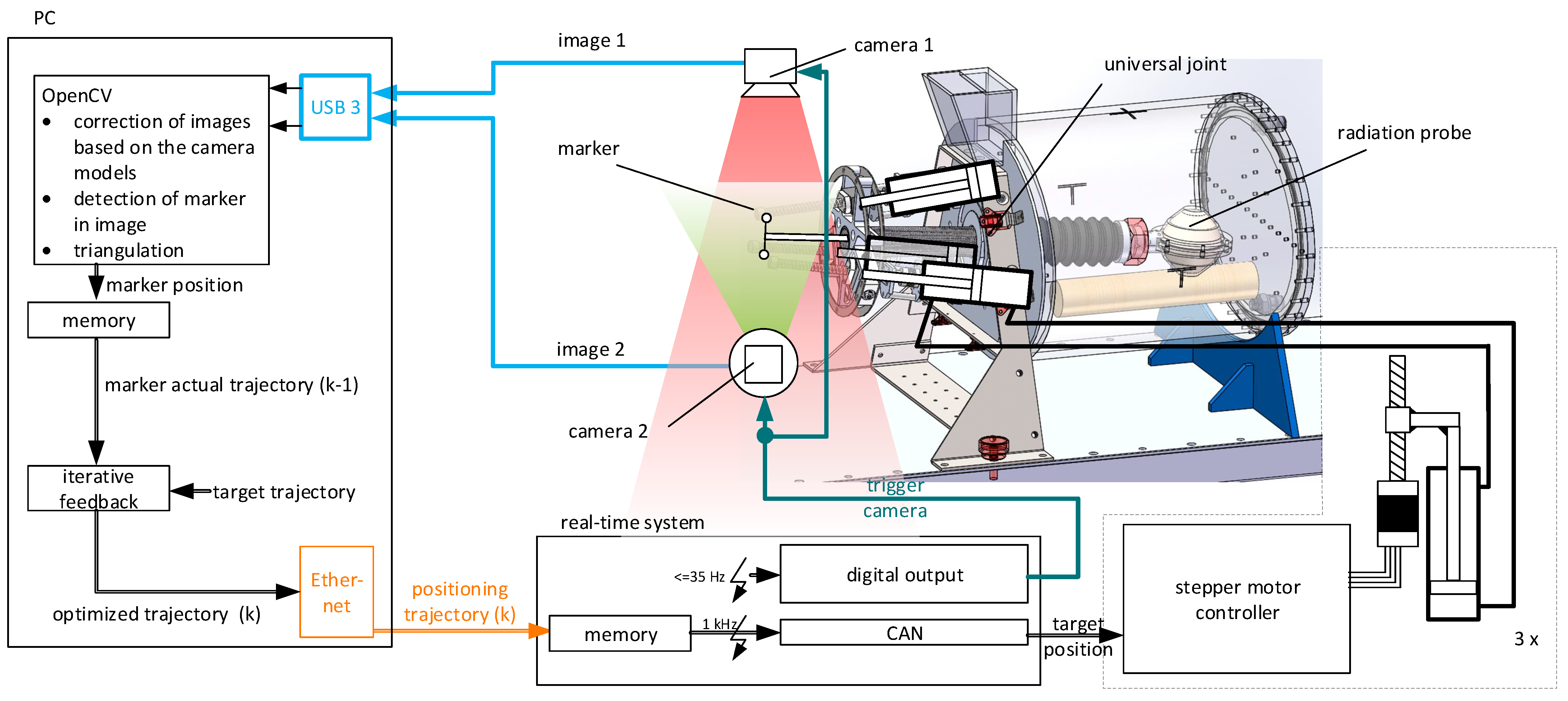
Figure 2 shows the desired principle of error correction and control of the MRI-compatible phantom prototype. The robot’s motion is defined by the three-arm parallel kinematics, actuated via slave hydraulic cylinders. A universal joint bears the rigid rod, on which the radiation probe and photogrammetric markers are placed at each end. This leads to three degrees of freedom: two rotations around, and one translation through the joint. The right-hand side is surrounded by a polymethyl methacrylate housing, wherein anthropomorphic tissue simulating objects can be placed. Since these objects would obstruct photogrammetric measurements, the camera system is placed on the left-hand side, where a free view on the rod can be guaranteed. Due to cameras in general not being MRI-compatible, the photogrammetric system is detachable from the robotic platform. This platform is designed to be mounted on the surgical table in any CT or MR device. This enables reevaluation of installed radiotherapy devices at hospitals.
A separate mobile device provides the hydraulic pressure via three master-cylinders, which are actuated by stepper motors via spindles. This device also contains the power electronics, controller hardware, storage space for the hose, and serves as a cart to transport the robot. For controlling the master cylinders’ movements and for synchronizing the camera shutters, a real-time system is used. A separate standard PC serves for computationally intensive tasks, such as photogrammetric evaluations and the ILC.
The robot’s trajectory evaluation is performed in two steps. First, a stereo camera module is mounted on the robot to measure the movement of a marker via photogrammetry. A desired synthetic trajectory like the one depicted in Figure 3 is provided and the required control signal is learned by the ILC. We use a synthetic trajectory throughout this paper as a development baseline; c.f. [10], for an analysis of real breathing patterns. In a second step, the non-MR-compatible camera module is removed and the radiation is activated. The radiation focus attempts to track the radiation probe along the learned trajectory. After that, the probe is analyzed to rate how well the radiation focus was following it.
3. Hydraulic Transmission
3.1. Concept
The basic concept is similar to that described in [14,15]. A master cylinder is connected via a hose to a slave cylinder. The master cylinder may be made of metal and may be operated with standard electromagnetic drive technology due to its location in the separated observation room. In contrast, the slave cylinder has to be made of specific plastics to ensure MR-compatibility and is mounted at the robot inside the hazardous measuring room, as depicted in Figure 4. Due to the hydraulic pressure, the slave experiences a driving force that depends on the movement of the master. The pre-pressurized fluid in the lines ensures that the delay in power transmission is less than that in open hydraulic systems with pump and control valves [17]. Therefore, it is assumed that the achievable stiffness is significantly higher than with open systems. Such a transmission allows high forces to be transmitted over long distances. The power-to-weight ratio of the slave cylinder is more favorable than for a linear motor placed at this point.
The comparable hydraulic transducer presented in [15] consists of a commercial master cylinder. The slave cylinder is a complex, MR-compliant special design made of polyethylene terephthalate. Both have a double-sided piston rod and, thus, additional seals and increased friction compared to cylinders with a single-sided piston rod. The system dynamics are only characterized for a single axis. Even though no quantification of the error was performed, the diagrams suggest significant deviations between the desired and actual trajectory.
3.2. Design and Setup
For the hydraulic transmission developed in this paper, cylinders with single-sided pistons are chosen and are operated in a closed circuit, which requires the same cross-section areas on each connected side of a piston. This design makes it possible to use inexpensive pneumatic components whose material properties were deemed sufficient for the setup with water filling. Water was preferred to oil as a hydraulic medium due to its easier handling in case of leakage at the experimental stage.
A norm cylinder ISO 15552 [19] with 50 mm piston diameter was used for the master cylinder. The plastic slave cylinder is also an ISO 15552 cylinder, manufactured by PSK Ingenieurgesellschaft mbH (Weimar, Germany). With a cylinder diameter of 50 mm and a piston rod diameter of 20 mm, the force of 531 N required for the application is achieved at a maximum pressure of 3.2 bar. The hoses are filled with a pre-pressure of 2 bar to pre-tension their elasticity. The components used have a permissible operating pressure of 10 bar. This leaves a safety limit of 4.8 bar for friction present in the system and any additional drive power required for the new robot design. The maximum achievable force in both directions with this transmission is 1600 N. In order to be able to vary the output force, the slave cylinder is coupled via a load cell to another pneumatic cylinder, which is equipped with throttles.
The cylinders are coupled with exchangeable plastic hose lines from Festo SE & Co. KG (Esslingen am Neckar, Germany) intended for pneumatics, which are also approved for use with water and have a diameter of 12 mm and a length of 10 m. Special attention was paid to low air bubble filling and the design of venting mechanisms of the closed hydraulic system. Residual air bubbles lower the stiffness and increase the stick-slip behavior, which was observed after incorrect venting or in longer durations between venting and measurement.
The process for stepper motor control and measurement data acquisition runs on the real-time system ADwin Gold II from Jäger Computergesteuerte Messtechnik GmbH (Lorsch, Germany). A CAN interface with CANopen protocol transmits the target motor positions from the real-time system to a stepper motor controller. A standard PC serves as a development environment in addition to image processing and as a user interface during operation (c.f. Figure 2). The target motor positions are transmitted at 1 kHz, the maximum possible rate of the motor controller used. In addition to the camera measuring system, the actual positions of the pistons are measured with interferometers at the master and slave cylinders, also at a 1 kHz sampling rate.
3.3. Validation
Figure 5 shows the path of the uncontrolled slave cylinder compared to the target position in a sinusoidal trajectory with a stroke of 50 mm, measured with a laser interferometer. Unwanted natural resonances of the system are mainly caused by the elasticity of the hoses. Even with a hose length of 10 m, the maximum deviation is significantly less than 1 mm and, thus, below the resolution of MRIs commonly in clinical use [5]. For the later robot construction, the use of metal-free high-pressure hoses with significantly higher rigidity is planned for improved accuracy. According to [9], this would already be sufficient for numerous MR-capable robots. For the planned application in the phantom and demanded deviations in the range of 200 µm, however, the accuracy of the test setup is not yet sufficient and is to be further improved with an ILC and photogrammetric measurements.
4. Photogrammetric Measurement System
The measurement system is intended to provide positional as well as orientational information of the phantom’s radiation probe by tracking the movement of the robot’s actuation side, as depicted in Figure 2. Since the correlation between the marker’s and the target’s movements are known by the kinematics of the robot, a direct photogrammetric measurement of the radiation probe can, thus, be avoided, which would be challenging due to the surrounding tissue-simulating obstacles (c.f. Figure 1). The spatial conversion from the tracked marker point to the radiation probe can then be achieved via geometrical relations of the robot known from mechanical design. As a drawback, this exhibits new sources of error due to the mechanical tolerances or clearance, which have to be addressed in the robot’s design.
In order to fulfill the accuracy demands on the total system, including ILC and construction tolerances, the measurement system itself must provide data of low noise and low repeatability error with estimated resolutions of 50 µm for a movement range of 8 cm in each spatial direction. A sampling rate and, therefore, frame rate of the cameras, of 25 Hz is seen as sufficient for the breathing movement trajectory, as shown in Figure 3.
4.1. Mathematical Characterization
Figure 6 shows a mathematical representation of a stereo camera system with its parameters, variables, and coordinate systems. The projection mechanism is modeled as a pinhole camera [20], with an assumed aperture of zero, so that no depth of field is considered and, thus, each image point corresponds to an object space ray. Therefore, each camera performs a projection of the three-dimensional world, including the robot’s markers, into a two-dimensional image plane, with the camera matrix
representing the projection parameters of camera i. Herein, are the focal lengths for each two-dimensional image plane coordinate, while and determine the image’s center. Additionally, the radial , as well as the tangential optical distortions of the image plane caused by the camera lens are taken into account [21]. The radial distortions are considered up to an order of 3, as higher-order corrections did not result in significantly better results in the case of higher-grade industry lenses.
Since each camera i has its own projection center denoted by the camera coordinate system , the relative pose between the cameras is defined by the rotation R and the translation T. If measurement results are to be expressed in a separate world coordinate system, additional relations between the cameras and the world coordinate system have to be introduced similarly. In this paper, we assume the projection center of camera 0 to represent the world coordinate system.
All these parameters have to be identified (c.f. Appendix A regarding the wording used here) by finding relations between the object and image space through the use of specific patterns, like, e.g., chessboards. For this, an optimization problem under variation of the unknown parameters is solved with the objective of minimizing projection errors, which is well-described in the literature [21,22,23]. In tests performed here, we used a chessboard pattern with approx. 5 to 10 taken single-view images per camera and around 15 images for both cameras. For the correct identification of distortions, it was crucial to place the chessboard pattern at least once in all four corners of each camera view. The obtained reprojection errors, which estimate the identification quality, varied around the value of 0.5 pixels.
4.2. Selection of Camera Components
For the photogrammetric system, a two-camera setup is chosen. While the addition of more cameras is likely to reduce stochastic errors, it increases the costs, complexity, and computational effort, as well as the extent of the measurement system. These cameras are mounted on a frame, which can then be temporarily attached to the phantom.
For the choice of the cameras, consumer webcams are a cheap option for high-resolution digital imaging and are used in various scientific photogrammetry projects [24,25] with sufficient accuracy. However, these cameras are usually found to exhibit several drawbacks for application to this robot:
- Lack of raw data access, as most webcams include algorithms for noise reduction, image sharpening, etc., which introduces systematic errors on the marker’s detection.
- Missing possibility to determine and fix camera parameters, like the focal length, focus, gain, aperture, and exposure.
- Rolling-shutter instead of global-shutter sensors lead to parallelogram-shaped distortions under moving scenery.
- Lack of synchronization between the two cameras’ exposure times limits the applicability for measuring moving objects.
Therefore, industrial cameras are used which overcome these limitations. In order to choose the correct camera sensor, a minimum pixel resolution has to be determined. With an estimated object space of , the given accuracy demand of µm, and a pessimistically estimated sub-pixel marker detection accuracy of , one obtains a minimum resolution of
Depending on the marker type and the detection algorithm, sub-pixel detection accuracies far below are reported [21,27], which is why cameras with cheaper image sensors and, therefore, lower resolutions could also perform as expected. However, a camera sensor with pixels was used for this work.
The lenses were chosen in a corresponding class of optical resolution, fitting to the 5 MP digital resolution. The focal length was selected according to the desired object distance and corresponding field of view. Since marker movements in the camera’s z-direction are also taking place, low apertures are beneficial in order to minimize varying marker sharpness due to the depth of field. The resulting photogrammetric module is shown in Figure 8.
In photography, the image’s lighting is determined by the three parameters of aperture, sensor gain, and exposure time. In order to achieve sharp images with low noise and low motion blur considering marker movements under exposure, all of these parameter values should be kept low, as long as the image lighting is acceptable. Additional light sources are an easy way to enhance these margins. The aperture’s influence on the depth of field as well as the effect of exposure time on motion blur can be calculated a priori, while the noise-inducing sensor gain should be tested experimentally. With bright marker illumination, the exposure times are of the order of 10 ms and, therefore, do not induce significant motion blur.
4.3. Selection of Photogrammetric Markers
The main demand on the marker is to enable automated and robust detection with high sub-pixel accuracy. The selection of appropriate markers is, therefore, closely related to the specific detection algorithms described in the literature and implemented in various computer vision libraries. For application in this project, various marker types were tested, including spheres and phosphorescent, markers as well as 2D patterns under various lighting conditions, such as background illumination or direct lighting. Most of these were found to be sensitive to the lighting conditions, camera adjustments or movement of the marker, also including false-positive results. For instance, the detection results of spheres via circle Hough transform depend on the parameters for the algorithm’s sensitivity as well as on the lighting of these spheres, and are, therefore, not robust enough for the desired application under the various lighting conditions in the radiotherapy room.
In contrast, chessboard patterns and their corresponding detection algorithms were found to exhibit high reproducibility, high detection rates, and close to zero false-positive results under varying lighting conditions, even with very small-sized projections of the chessboard. Typical detection algorithms recognize all of the pattern’s inner corners, and are, thus, able to reduce the stochastic error due to image noise by averaging the 3D positions of all these interest points.
In the literature, chessboard patterns are mostly proposed as a pattern for performing camera parameter identification [24,28,29]. However, in this paper, the chessboard pattern is directly used as the photogrammetric target marker. The pattern is thereby printed with a conventional laser printer and glued onto a flat plastic board. Further improvement could be achieved with different printing procedures of higher resolution. Also, laser-printed surfaces are known for their reflections, which has to be considered with the additional lighting.
4.4. Software Implementation
The implementation is performed in Python 3.11.4 with the help of the OpenCV 4.8.1.78 library (via opencv-python) for the computer vision parts. Since detection of chessboard patterns is time-consuming on larger images [21] and live-tracking of the marker positions without storing the camera frames should be enabled, a parallelized approach, as depicted in Figure 9, is used. Herewith, a complete photogrammetrical live evaluation of 5 MP-sized frames can be achieved with a frequency of approx. 30 Hz on a standard PC (tested on an AMD Ryzen 3600XT CPU with 16 GB DDR4-3200 RAM and Windows 10 22H2).
In a similar way, a method for identification of the camera parameters is implemented, which enables detection of the chessboard pattern for both cameras simultaneously. The detected chessboard positions during all the different chessboard poses are then sorted for use in the camera-specific identification as well as for the relative pose estimation. For that, the OpenCV calibrateCamera() and stereoCalibrate() methods are used and additional parameters, like projection matrices, are calculated. After that, all the identification results are saved in files, which will be used in the following measurement runs.
4.5. Validation of Reached Accuracy
For validation of the photogrammetric system, the test bench shown in Figure 10 was built up. It combines a linear bearing with actuation and a laser interferometer. On the slide, a chessboard pattern is mounted, which is observed by two stationary cameras at a relative angle of approx. 90°. The interferometer enables measurements of the linear movement with far higher accuracy than the photogrammetric system and is, therefore, capable of validation of the photogrammetric setup. In the case of the 3D photogrammetric measurement system, the Euclidean distance from the starting point is taken for comparison. For each step in position, ten measurement samples are obtained.
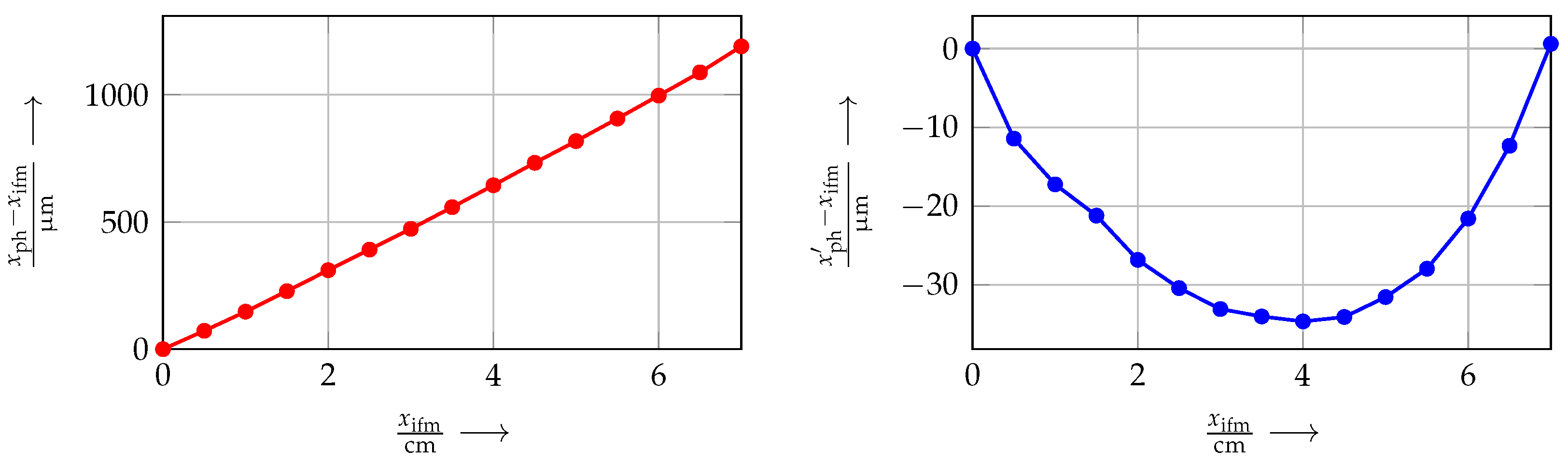
Figure 11 shows the results of this validation. Along the tested movement range of 7 cm, a maximum deviation between the photogrammetric system and the interferometer of 1190 µm can be observed, when the starting points of both systems are assumed to be zero. The mainly linear shape of the measurement deviation leads to the assumption that a constant scaling factor for camera parameter identification is off-size. This can be found in the length of a chessboard tile, which is a linear scaling parameter for the total system identification process and was only measured by a sliding caliper. After a correction of this by a factor of 1190 µm/7 cm, the systematic error of the photogrammetric system can be reduced to 35 µm. Due to its shape, the remaining errors are likely to come from over- or under-corrected optical distortions, which could be further decreased by putting more effort into the camera identification process prior to the measurement.
Mainly due to image noise, stochastic errors also occur. For the ten measurement samples per position, the median of these errors is estimated as u = 0.311 µm, which is far below the desired measurement accuracies. This, in total, enables the photogrammetric system to perform measurements for the described robotic phantom. The exact error quantities for the application depend on different factors, like the lighting and the field of view; however, only small deviations from the investigated errors are to be expected during application, as long as photogrammetric identification is performed accurately.
5. Iterative Learning Control
The distance between the measurement and observation rooms can be several meters, resulting in long hoses. This adds considerable inertia and lowers the transmission stiffness. Low stiffness in combination with friction of the pistons makes control challenging due to the stick-slip effect [14]. The transmission behavior of the system under consideration is clearly non-linear, which makes it difficult to design a stable control system. ILCs are not closed-loop-control methods, but rather involve open-loop-control with section-by-section adjustment of the control signal. Since the required trajectories of the robotic phantom are periodic, giving a repeated motion, an ILC deployment was deemed appropriate to control the slave-pistons at a high level of accuracy.
The idea is to compare the slave piston position from a previous period to the target trajectory. The new control input is then iteratively calculated from the previous input and the current trajectory error. Thus, the control input is adjusted with each period for increasing accuracy [30]. This approach is also advantageous due to the position information gathered by the photogrammetric system being delayed by the computation time, which is usually in the region of . This significant delay or dead time would otherwise be a problem for closed-loop-control methods.
5.1. System Dynamics Model
The ILC design is based on a simulation of the dynamic behavior of the system. Two different approaches were used to derive models for the individual system components from the system shown in Figure 12. In the first approach, a multi-domain model for describing the system behavior was set up by linking the fluid-mechanic equations of the individual components. Apart from consideration of the masses, transmission stiffnesses, and the piston as a domain-linking component, the hydraulic system itself is represented by a combination of capacitive elements for the hoses’ stiffnesses and hydraulic inertia to represent the water mass inside the hoses. For coverage of oscillatory effects, a discretization of the inertia and capacitance over the hose length is considered. This physical model was examined for hose models with discretizations of one and three.
In a second approach, the hydraulic components were directly modeled as mechanical springs, dampers, and masses, based on the analogy between hydraulic and mechanical effects. The results of this abstraction are two-mass and three-mass oscillators to be investigated as potential system models. Both phenomenological models are shown in Figure 13.
When validating the physical as well as the phenomenological models and their variants, it was shown that no significant improvement in model accuracy was achieved either by three discretizations of the hose or by expanding from a two- to a three-mass oscillator. For 5 m hose assemblies, the four models investigated achieve an accuracy of approx. 0.3 mm for a movement over 150.0 mm compared to measurements on the real system, which is shown in Figure 14. When simulating the same model with a hose length of 10 m, it became clear that none of the models could reproduce the internal vibration behavior of the system, which increases with the hose length, to a satisfying degree for ILC deployment. The accuracy of the best model compared to reality is reduced to 1.0 mm over 150.0 mm.
Despite significantly lower system order and complexity, the models of the second approach reproduce the system behavior with similar accuracy. Due to the lower system order with comparable accuracy, the two-mass oscillator was selected as the system model for the following ILC design. The model contains masses and for each piston, including parts of the water mass inside the hose, and the hydraulic stiffness of the hose on the right-hand side. To the left, PT1 and represent the stepper motor dynamic and spindle stiffness, respectively.
5.2. ILC Design
Two simulation-based ILC procedures were designed. For the PD-ILC, recommended in [30], a parameter set was determined experimentally. Similar to their closed-loop counterparts P-, D-, and PD-ILC are composed of a proportional and, if necessary, a differential component, if applicable. The extension by a dedicated integral component is unusual since the ILC control law itself already leads to an integration over each iteration [31].
For the design of a plant-inversion ILC, a calculation rule for the numerical inversion of the two-mass oscillator model was implemented.
By simulating both ILC variants, their suitability for controlling the system model was confirmed. However, when transferring the designed ILC to the real test setup with long hose lines, it was found that the accuracy of the system model was not sufficient for designing the ILC by simulation. Due to only partial coverage of oscillatory behavior in the system model, none of the ILC designs could reliably control the real system. However, the numerical inversion of the system model from the plant inversion ILC is suitable for calculating an initial guess trajectory for the PD-ILC. Based on this, a combined procedure of feed-forward control by the inverse model and PD-ILC was chosen for the further approach.
The resulting control law of the PD-ILC is
The new control trajectory is calculated from the former trajectory and the deviation between the actual and the desired trajectory for each time step k, multiplied by P- and D-factors and , respectively. The trajectory error for the P-component is evaluated at the future time step , since this was found to make the algorithm more numerically stable. A Gaussian function for smoothing the differential component was added.
For systems with time-delaying components like the one described in this paper, a time-shift d has to be included in the control law. The reason for this is that in the case of a pure P-ILC, it can be observed that the error at the slave cylinder decreases over a certain number of learning steps and then starts increasing again. This happens due to an increasing oscillation at the output, which cannot be compensated by the ILC, since time-delaying effects make the total system oscillatory. Due to the time-delaying effects, the corrective intervention of the ILC does not act at the time of the cause of the deviations. To prevent this, for the calculation of at time step k, the error is additionally time-shifted by the integer relative dead time factor d [32]. The factor d can be estimated on the basis of the periodic time of the resulting oscillation T in relation to the sampling time of the ILC. Good results were obtained with .
A parameter set for controlling the real setup with long hose assemblies was experimentally determined. The first step is the identification of the relative dead time factor using a P-ILC () with arbitrarily chosen and . In our case, the upcoming oscillation had a period duration of and the sampling time is , which leads to a relative dead time factor . In the next step, is chosen in a way that the error during learning quickly becomes small under the constraint of non-observable oscillations (in our case ). In the same way was determined.
5.3. Validation
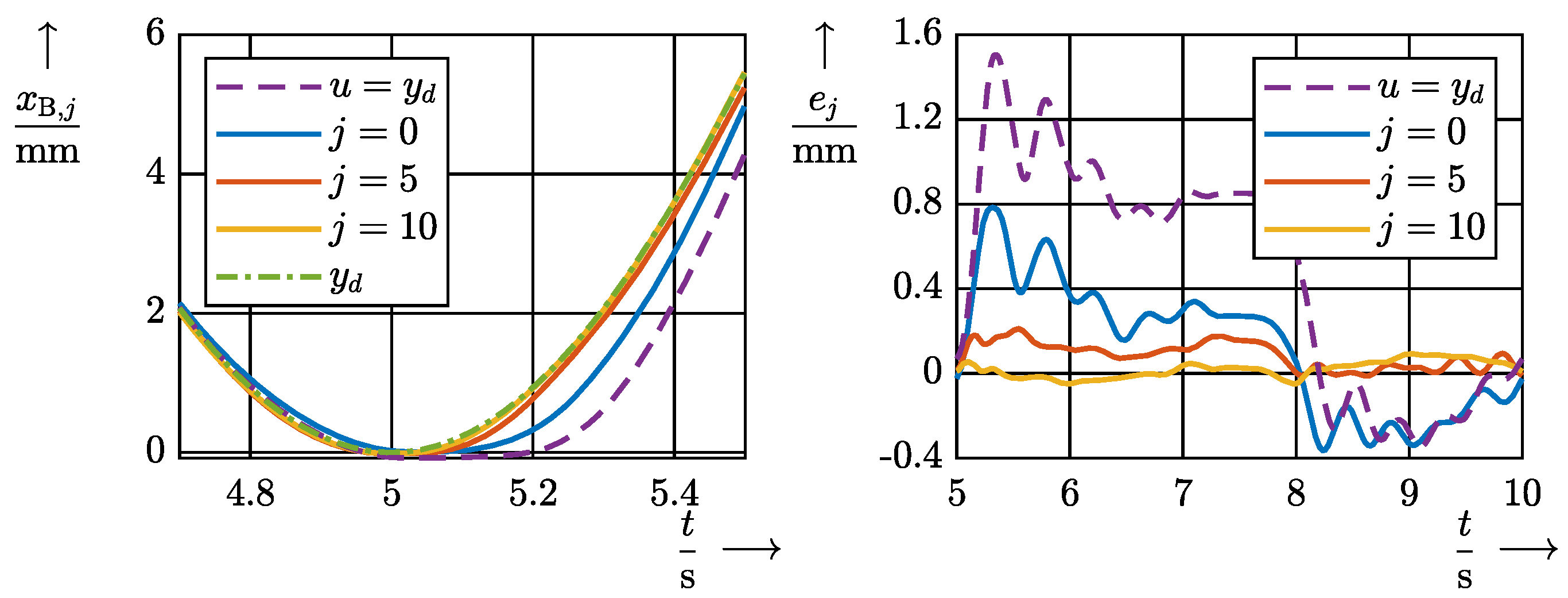
Figure 15 on the right shows the resulting ILC of the breathing movement from Figure 3, reducing the maximum error of the system below 100 µm within 10 iterations. The reproducibility of the learning process was confirmed by multiple repetitions. Figure 16 on the left shows the course of the maximum error for several learning processes carried out in succession. The deviation at repetition three occurs at the first points of the trajectory due to stronger static friction. In principle, all the repetitions show a similar course.
Finally, the re-usability of the obtained actuator trajectory was investigated. The master cylinder was repeatedly moved with a learned control sequence without relearning it. The trajectory of the slave cylinder changes only slightly. Figure 16 on the right shows the maximum error for 10 repetitions of the control sequence. By applying this learned trajectory to the real system, a maximum deviation of 130 µm was reliably achieved in the repetitions. It can be concluded that the system behavior is strongly non-linear but reproducible. Trajectories of different shape with similar dynamics are expected to be reproduced with similar accuracy.
6. Conclusions
In this paper, the development, measurement, and control of a single-axis actuation system was investigated, which can be used for a robotic phantom for radiotherapy device evaluation. For this, an MR- and radiation-compatible hydraulic transmission was built up and tested for remote actuation from outside the MRI, which was found to be appropriate for the desired application. Measurement of the system’s position was carried out with a detachable stereo camera pair observing a chessboard pattern as the target marker, which allows 3D positional measurements with a low systematic error of 35 µm, as well as very low noise in the region of µm. The photogrammetric accuracy can be further increased by selecting cameras with higher digital resolution and lenses with higher optical resolution. Calibrating the photogrammetric system against a measurement system of higher accuracy and adjusting the resulting measurement values can additionally be used to compensate systematic errors.
The residual errors of the actuation system, mainly caused by cylinder friction in combination with compressibility of the fluid and hoses, are shown to be minimizable by the suggested ILC up to a remaining maximum error of 130 µm. Thereby, the proposed procedures offer an advantage over the usual purely model-based control and can substitute for a closed loop control. Due to the ILC mainly compensating errors from friction and oscillations, our expectation is that applying different, more realistic human movement patterns will lead to errors of comparable size.
Future work will address integrating the 1D actuation concept in the robotic phantom as well as testing the photogrammetry and ILC in 3D on the final system. Additional clinical tests will assess the applicability for the desired purpose of radiotherapy device validation in MRI environments with different patient-specific phantom movement trajectories. Additional accuracy improvements regarding the uncontrolled hydraulic transmission can be made using non-conductive high-pressure hydraulic hoses with aramid reinforcement and, therefore, higher stiffness in order to reduce oscillatory errors. In order to determine the cut-off frequency of the developed actuation system, which limits the reproducible trajectory dynamics, the frequency response characteristic should also be measured.
Author Contributions
Conceptualization, O.R. and T.S.; methodology, J.M., O.R., and T.S.; software, J.M. and O.R.; validation, J.M. and O.R.; formal analysis, J.M. and O.R.; investigation, J.M. and O.R.; resources, T.S.; data curation, J.M. and O.R.; writing—original draft preparation, J.M. and O.R.; writing—review and editing, J.M., O.R. and T.S.; visualization, J.M. and O.R.; supervision, T.S.; project administration, O.R. and T.S.; funding acquisition, O.R. and T.S. All authors have read and agreed to the published version of the manuscript.
Funding
This research was funded by Bundesministerium für Bildung und Forschung (BMBF, Federal Ministry of Education and Research) within research initative “KMU-innovativ: Medizintechnik” under grant number 13GW0351B. Collaborating project partners are Boll Automation GmbH (Kleinwallstadt, Germany) and Deutsches Krebsforschungszentrum (Heidelberg, Germany). We acknowledge support for the publication costs by the Open Access Publication Fund of the Technische Universität Ilmenau.
Data Availability Statement
The raw data supporting the conclusions of this article will be made available by the authors on request.
Acknowledgments
The authors thank Martin Dahlmann (Mechatronics Group, Technische Universität Ilmenau) for discussions, ideas and review of the project. The authors also thank René Beck and Alexander Jurin (both students at Mechatronics Group, Technische Universität Ilmenau) for supplementary work on the ILC implementation as well as help on the photogrammetrical test setup, respectively. The photograph of Figure 1 was taken by Felix Hähn from our project partner Boll Automation GmbH (Kleinwallstadt, Germany).
Conflicts of Interest
The authors declare no conflicts of interest.
Abbreviations
The following abbreviations are used in this manuscript:
| CT | Computed tomography |
| ILC | Iterative learning control |
| MRI | Magnetic resonance imaging |
Appendix A. Wording: Camera Calibration vs. Identification
In photogrammetry, the identification process of intrinsic and extrinsic camera parameters is often referred to as camera calibration [21,22,23]. However, since no actual calibration in terms of measurement technology is performed [33], the term is considered misleading by the authors. Therefore, in this paper, this process is called identification.
References
- Bergeles, C.; Yang, G.Z. From Passive Tool Holders to Microsurgeons: Safer, Smaller, Smarter Surgical Robots. IEEE Trans. Biomed. Eng. 2014, 61, 1565–1576. [Google Scholar] [CrossRef]
- Burgner-Kahrs, J.; Rucker, D.C.; Choset, H. Continuum Robots for Medical Applications: A Survey. IEEE Trans. Robot. 2015, 31, 1261–1280. [Google Scholar] [CrossRef]
- Vitiello, V.; Lee, S.L.; Cundy, T.P.; Yang, G.Z. Emerging Robotic Platforms for Minimally Invasive Surgery. IEEE Rev. Biomed. Eng. 2013, 6, 111–126. [Google Scholar] [CrossRef] [PubMed]
- Panfili, E.; Pierdicca, L.; Salvolini, L.; Imperiale, L.; Dubbini, J.; Giovagnoni, A. Magnetic resonance imaging (MRI) artefacts in hip prostheses: A comparison of different prosthetic compositions. Radiol. Medica 2014, 119, 113–120. [Google Scholar] [CrossRef] [PubMed]
- Tsekos, N.V.; Khanicheh, A.; Christoforou, E.; Mavroidis, C. Magnetic Resonance–Compatible Robotic and Mechatronics Systems for Image-Guided Interventions and Rehabilitation: A Review Study. Annu. Rev. Biomed. Eng. 2007, 9, 351–387. [Google Scholar] [CrossRef] [PubMed]
- Herl, G.; Hiller, J.; Sauer, T. Artifact reduction in X-ray computed tomography by multipositional data fusion using local image quality measures. In Proceedings of the 9th Conference on Induatrial Computed Tomography, Padova, Italy, 13–15 February 2019. [Google Scholar] [CrossRef]
- Mühlenhoff, J.; Körbner, T.; Miccoli, G.; Keiner, D.; Hoffmann, M.K.; Sauerteig, P.; Worthmann, K.; Flaßkamp, K.; Urbschat, S.; Oertel, J.; et al. A manually actuated continuum robot research platform for deployable shape-memory curved cannulae in stereotactic neurosurgery. In Proceedings of the ACTUATOR 2022: International Conference and Exhibition on New Actuator Systems and Applications, Mannheim, Germany, 28–30 June 2022; pp. 1–4. [Google Scholar]
- Winkel, D.; Bol, G.H.; Kroon, P.S.; van Asselen, B.; Hackett, S.S.; Werensteijn-Honingh, A.M.; Intven, M.P.; Eppinga, W.S.; Tijssen, R.H.; Kerkmeijer, L.G.; et al. Adaptive radiotherapy: The Elekta Unity MR-linac concept. Clin. Transl. Radiat. Oncol. 2019, 18, 54–59. [Google Scholar] [CrossRef] [PubMed]
- Monfaredi, R.; Cleary, K.; Sharma, K. MRI robots for needle-based interventions: Systems and technology. Ann. Biomed. Eng. 2018, 46, 1479–1497. [Google Scholar] [CrossRef]
- Arenbeck, H. Robotische Systeme und Regelungsstrategien für die Radiotherapie bewegter Tumore. Ph.D. Thesis, RWTH Aachen, Aachen, Germany, 2015. [Google Scholar]
- Arenbeck, H.; Prause, I.; Abel, D.; Corves, B. Development and Analysis of a Novel Parallel Manipulator Used in Four-Dimensional Radiotherapy. J. Mech. Robot. 2017, 9, 031006. [Google Scholar] [CrossRef]
- Dunn, L.; Kron, T.; Johnston, P.; McDermott, L.; Taylor, M.; Callahan, J.; Franich, R. A programmable motion phantom for quality assurance of motion management in radiotherapy. Australas. Phys. Eng. Sci. Med. 2012, 35, 93–100. [Google Scholar] [CrossRef] [PubMed]
- Ranjbar, M.; Sabouri, P.; Repetto, C.; Sawant, A. A novel deformable lung phantom with programably variable external and internal correlation. Med. Phys. 2019, 46, 1995–2005. [Google Scholar] [CrossRef] [PubMed]
- Ganesh, G.; Gassert, R.; Burdet, E.; Bleuler, H. Dynamics and control of an MRI compatible master-slave system with hydrostatic transmission. In Proceedings of the IEEE International Conference on Robotics and Automation, New Orleans, LA, USA, 26 April–1 May 2004; Volume 2, pp. 1288–1294. [Google Scholar] [CrossRef]
- Gassert, R.; Moser, R.; Burdet, E.; Bleuler, H. MRI/fMRI-compatible robotic system with force feedback for interaction with human motion. IEEE/ASME Trans. Mechatron. 2006, 11, 216–224. [Google Scholar] [CrossRef]
- Yu, N.; Riener, R. Review on MR-Compatible Robotic Systems. In Proceedings of the First IEEE/RAS-EMBS International Conference on Biomedical Robotics and Biomechatronics (BioRob), Pisa, Italy, 20–22 February 2006; pp. 661–665. [Google Scholar] [CrossRef]
- Yu, N.; Hollnagel, C.; Blickenstorfer, A.; Kollias, S.S.; Riener, R. Comparison of MRI-Compatible Mechatronic Systems with Hydrodynamic and Pneumatic Actuation. IEEE/ASME Trans. Mechatron. 2008, 13, 268–277. [Google Scholar] [CrossRef]
- Tijssen, R.H.; Philippens, M.E.; Paulson, E.S.; Glitzner, M.; Chugh, B.; Wetscherek, A.; Dubec, M.; Wang, J.; van der Heide, U.A. MRI commissioning of 1.5T MR-linac systems—A multi-institutional study. Radiother. Oncol. 2019, 132, 114–120. [Google Scholar] [CrossRef]
- DIN ISO 15552:2005-12; Pneumatik Fluid Power—Cylinders with Detachable Mountings, 1000 kPa (10 bar) Series, Bores from 32 mm to 320 mm–Basic, Mounting and Accessories Dimensions. Deutsches Institut für Normung: Berlin, Germany, 2005. [CrossRef]
- Hartley, R.; Zisserman, A. Multiple View Geometry in Computer Vision, 2nd ed.; Cambridge University Press: Cambridge, UK, 2004. [Google Scholar] [CrossRef]
- Duda, A.; Frese, U. Accurate Detection and Localization of Checkerboard Corners for Calibration. In Proceedings of the 29th British Machine Vision Conference, Newcastle, UK, 3–6 September 2018. [Google Scholar]
- Wang, Y.M.; Li, Y.; Zheng, J.B. A camera calibration technique based on OpenCV. In Proceedings of the 3rd International Conference on Information Sciences and Interaction Sciences, Chengdu, China, 23–25 June 2010; pp. 403–406. [Google Scholar] [CrossRef]
- Datta, A.; Kim, J.S.; Kanade, T. Accurate camera calibration using iterative refinement of control points. In Proceedings of the IEEE International Conference on Computer Vision Workshops, Kyoto, Japan, 27 September–4 October 2009; pp. 1201–1208. [Google Scholar] [CrossRef]
- Greiner-Petter, C.; Sattel, T. On the influence of pseudoelastic material behaviour in planar shape-memory tubular continuum structures. Smart Mater. Struct. 2017, 26, 125024. [Google Scholar] [CrossRef]
- Watts, T.; Secoli, R.; y Baena, F.R. A Mechanics-Based Model for 3-D Steering of Programmable Bevel-Tip Needles. IEEE Trans. Robot. 2019, 35, 371–386. [Google Scholar] [CrossRef]
- USB Implementers Forum. Universal Serial Bus Device Class Definition for Video Devices, Revision 1.5. 2012. Available online: https://www.usb.org/document-library/video-class-v15-document-set (accessed on 17 February 2024).
- Yao, L.; Liu, H. A Flexible Calibration Approach for Cameras with Double-Sided Telecentric Lenses. Int. J. Adv. Robot. Syst. 2016, 13. [Google Scholar] [CrossRef]
- Strobl, K.H.; Hirzinger, G. More accurate pinhole camera calibration with imperfect planar target. In Proceedings of the IEEE International Conference on Computer Vision Workshops, Barcelona, Spain, 6–13 November 2011; pp. 1068–1075. [Google Scholar] [CrossRef]
- Wohlfeil, J.; Grießbach, D.; Ernst, I.; Baumbach, D.; Dahlke, D. Automatic camera system calibration with a chessboard enabling full image coverage. Int. Arch. Photogramm. Remote Sens. Spat. Inf. Sci. 2019, 42, 1715–1722. [Google Scholar] [CrossRef]
- Bristow, D.; Tharayil, M.; Alleyne, A. A survey of iterative learning control. IEEE Control Syst. Mag. 2006, 26, 96–114. [Google Scholar] [CrossRef]
- Ahn, H.S.; Chen, Y.; Moore, K.L. Iterative Learning Control: Brief Survey and Categorization. IEEE Trans. Syst. Man Cybern. Part C (Appl. Rev.) 2007, 37, 1099–1121. [Google Scholar] [CrossRef]
- Chen, C.K.; Zeng, W.C. The Iterative Learning Control for the Position Tracking of the Hydraulic Cylinder. JSME Int. J. Ser. C Mech. Syst. Mach. Elem. Manuf. 2003, 46, 720–726. [Google Scholar] [CrossRef]
- ISO/IEC Guide 99:2007; International vocabulary of metrology—Basic and general concepts and associated terms (VIM). International Organization for Standardization: Geneva, Switzerland, 2010.
Figure 1.
MR-compatible prototype of a robotic phantom in a CT scanner with the parallel joint kinematics on the right, the transparent chamber filled with anthropomorphic structures in the middle, as well as the movable radiation probe inside of the chamber.
Figure 1.
MR-compatible prototype of a robotic phantom in a CT scanner with the parallel joint kinematics on the right, the transparent chamber filled with anthropomorphic structures in the middle, as well as the movable radiation probe inside of the chamber.

Figure 2.
Error correction principle for the robotic phantom prototype, including hydraulic actuation, positional measurement via cameras, as well as positional control of the radiation probe.
Figure 2.
Error correction principle for the robotic phantom prototype, including hydraulic actuation, positional measurement via cameras, as well as positional control of the radiation probe.

Figure 3.
1D simulated example trajectory for a patient’s breathing movements of Hz frequency, which the robot should be able to follow (derived from [10]).
Figure 3.
1D simulated example trajectory for a patient’s breathing movements of Hz frequency, which the robot should be able to follow (derived from [10]).

Figure 4.
Principle of the hydraulic transducer.

Figure 5.
Left: target and actual position with sinusoidal actuation of the master piston with a hose length of 10 m. Right: deviation between target and actual position at the slave piston for different hose lengths.
Figure 5.
Left: target and actual position with sinusoidal actuation of the master piston with a hose length of 10 m. Right: deviation between target and actual position at the slave piston for different hose lengths.

Figure 6.
Mathematical description of the photogrammetric system. The target inside the object space (at the top) is projected to image spaces in each camera (left and right), which have their individual optical parameters.
Figure 6.
Mathematical description of the photogrammetric system. The target inside the object space (at the top) is projected to image spaces in each camera (left and right), which have their individual optical parameters.

Figure 7.
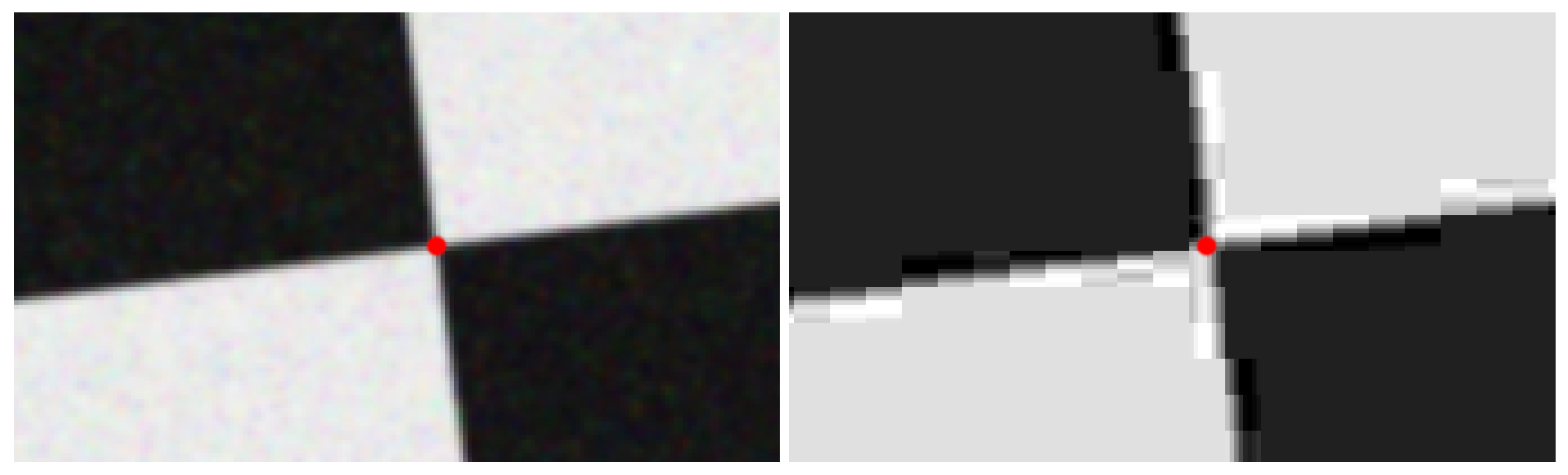
Effects of lossy compression (e.g., JPEG, quality level 0, right image) on the precise detection of markers using a synthetic chessboard image with noise (left image). Depending on starting point and search region, the chessboard corner refinement algorithm cornerSubPix() results in different pixel coordinates ( vs. for an initial guess of ).
Figure 7.
Effects of lossy compression (e.g., JPEG, quality level 0, right image) on the precise detection of markers using a synthetic chessboard image with noise (left image). Depending on starting point and search region, the chessboard corner refinement algorithm cornerSubPix() results in different pixel coordinates ( vs. for an initial guess of ).

Figure 8.
Photogrammetric system consisting of two 5 MP industrial cameras (Basler acA2440-35uc) with heat sinks for lowering sensor noise mounted on ball heads, corresponding 16 mm f/1.4 normal lenses (Ricoh FL-CC1614-5M), and a real-time controller (ADwin-Gold II) for synchronization of the camera shutters. The image data are transferred via USB3 Vision standard to a PC [7].

Figure 9.
Software architecture for parallelized chessboard searches. All worker methods run in separate Python processes (blue), while thread-safe queues (green) take care of data interchange. With that, frames of different time points are processed independently, increasing the computational speed.

Figure 10.
1D linear test setup for validating the accuracy of the photogrammetric system. On the upper right corner, the camera view during measurements, including the detection result, is shown.
Figure 10.
1D linear test setup for validating the accuracy of the photogrammetric system. On the upper right corner, the camera view during measurements, including the detection result, is shown.

Figure 11.
Measurement error between laser interferometer and photogrammetric system before (left) and after correction of the measured value for the chessboard size (right).
Figure 11.
Measurement error between laser interferometer and photogrammetric system before (left) and after correction of the measured value for the chessboard size (right).

Figure 12.
Basic system structure for the physical model.

Figure 13.
Phenomenological models for the hydraulic transmission: two-mass oscillator (left) and three-mass oscillator (right).
Figure 13.
Phenomenological models for the hydraulic transmission: two-mass oscillator (left) and three-mass oscillator (right).

Figure 14.
Left: master piston trajectory u for the simulations. Right: deviation between simulation and experiment for the physical and the phenomenological model for hose assemblies of 5 m.
Figure 14.
Left: master piston trajectory u for the simulations. Right: deviation between simulation and experiment for the physical and the phenomenological model for hose assemblies of 5 m.

Figure 15.
Left: cutout of the reached master piston trajectory with the target being denoted by for different steps of the ILC: without any ILC application, with only plant-inversion ILC, and the converging trajectories of the PD-ILC iterations j. Right: resulting errors.
Figure 15.
Left: cutout of the reached master piston trajectory with the target being denoted by for different steps of the ILC: without any ILC application, with only plant-inversion ILC, and the converging trajectories of the PD-ILC iterations j. Right: resulting errors.

Figure 16.
Left: development of the maximum error over ILC learning iterations j for different repetitions of the learning process applied to the identical system. Right: repeated application of the best control scheme, showing small deviations from run to run with a runaway value at .
Figure 16.
Left: development of the maximum error over ILC learning iterations j for different repetitions of the learning process applied to the identical system. Right: repeated application of the best control scheme, showing small deviations from run to run with a runaway value at .

Disclaimer/Publisher’s Note: The statements, opinions and data contained in all publications are solely those of the individual author(s) and contributor(s) and not of MDPI and/or the editor(s). MDPI and/or the editor(s) disclaim responsibility for any injury to people or property resulting from any ideas, methods, instructions or products referred to in the content. |
© 2024 by the authors. Licensee MDPI, Basel, Switzerland. This article is an open access article distributed under the terms and conditions of the Creative Commons Attribution (CC BY) license (https://creativecommons.org/licenses/by/4.0/).
Share and Cite
MDPI and ACS Style
Mühlenhoff, J.; Radler, O.; Sattel, T. Development of a Hydraulic Actuator for MRI- and Radiation-Compatible Medical Applications. Actuators 2024, 13, 90. https://doi.org/10.3390/act13030090
AMA Style
Mühlenhoff J, Radler O, Sattel T. Development of a Hydraulic Actuator for MRI- and Radiation-Compatible Medical Applications. Actuators. 2024; 13(3):90. https://doi.org/10.3390/act13030090
Chicago/Turabian StyleMühlenhoff, Julian, Oliver Radler, and Thomas Sattel. 2024. "Development of a Hydraulic Actuator for MRI- and Radiation-Compatible Medical Applications" Actuators 13, no. 3: 90. https://doi.org/10.3390/act13030090
Note that from the first issue of 2016, this journal uses article numbers instead of page numbers. See further details here.