Intelligent Fault Diagnosis Method through ACCC-Based Improved Convolutional Neural Network

Abstract

Fault diagnosis plays an important role in improving the safety and reliability of complex equipment. Convolutional neural networks (CNN) have been widely used to diagnose faults due to their powerful feature extraction and learning capabilities. In practical industrial applications, the obtained signals always are disturbed by strong and highly non-stationary noise, so the timing relationships of the signals should be highlighted more. However, most CNN-based fault diagnosis methods directly use a pooling layer, which may corrupt the timing relationship of the signals easily. More importantly, due to a lack of an attention mechanism, it is difficult to extract deep informative features from noisy signals. To solve the shortcomings, an intelligent fault diagnosis method is proposed in this paper by using an improved convolutional neural network (ICNN) model. Three innovations are developed. Firstly, the receptive field is used as a guideline to design diagnosis network structures, and the receptive field of the last layer is close to the length of the original signal, which can enable the network to fully learn each sample. Secondly, the dilated convolution is adopted instead of standard convolution to obtain larger-scale information and preserves the internal structure and temporal relation of the signal when performing down-sampling. Thirdly, an attention mechanism block named advanced convolution and channel calibration (ACCC) is presented to calibrate the feature channels, thus the deep informative features are distributed in larger weights while noise-related features are effectively suppressed. Finally, two experiments show the ICNN-based fault diagnosis method can not only process strong noise signals but also diagnose early and minor faults. Compared with other methods, it achieves the highest average accuracy at 94.78% and 90.26%, which are 6.53% and 7.70% higher than the CNN methods, respectively. In complex machine bearing failure conditions, this method can be used to better diagnose the type of failure; in voice calls, this method can be used to better distinguish between voice and noisy background sounds to improve call quality.

1. Introduction

In recent years, deep learning (DL) methods are increasingly used in fault diagnosis and prediction [1,2,3]. Deep learning is an algorithm based on data representation learning in machine learning. An intelligent diagnosis using deep learning gets rid of the dilemma that traditional fault diagnosis methods rely too much on diagnostics experts and professional technicians and breaks the deadlock between a large amount of diagnostic data for mechanical equipment and the relatively few diagnostic experts. Traditional machine learning techniques are limited in their ability to process natural data in its raw form. The most obvious difference between deep learning models and traditional models is that DL can learn the abstract representation features of the raw data automatically [4].

Several DL methods, such as the deep belief network (DBN), deep auto-encoder (DAE), and convolutional neural network (CNN) have been applied to fault diagnosis [5]. These three deep learning models are all built with different base models, and they all have their own characteristics in feature learning [6]. DAE is easy to train and is a pure unsupervised feature learning model [7]. DBN is a probabilistic generation model, which can obtain the joint distribution of observed data and markers [8]. CNN has some attractive advantages, such as shift-invariance and weight sharing [9]. Compared with the traditional machine learning method, DL has achieved good results, but its application in fault diagnosis is still in the development stage.

As one of the most effective DLs, CNNs have been widely used in image classification, object detection, and semantic segmentation. Gaurav Dhiman et al. proposed a method aimed at the characteristics of discrete attributes of tumor-related medical events and proposes a medical event [10]. CNN has the ability to represent learning and can shift invariant classification of input information according to its hierarchical structure. Therefore, it is also called “Shift - Invariant Artificial Neural Networks (SIANN)”. In the 21st century, with the proposal of DL theory and the improvement of numerical computing equipment, CNN has been rapidly developed, and has been applied to computer vision, natural language processing, and other fields. As a machine learning model under deep supervised learning, CNN has strong adaptability. It is good at mining local features of data and extracting global training features and classification. Its weight-sharing structure network makes it more similar to biological neural networks and has achieved good results in all fields of pattern recognition [11].

To further improve the performance of deep CNNs, many studies have been carried out since the pioneering Alex Net [12]. Long Wen et al. [13] built a new CNN based on LeNet-5 for fault diagnosis. Through a conversion method of converting signals into two-dimensional images, the proposed method can extract the features of the converted 2D images and eliminate the effect of handcrafted features. Zhao et al. [14] proposed a method to convert the one-dimensional vibration signals into two-dimensional grey images, and then 2D-CNN is used to extract fault features and realize fault classification. However, the conversion process of the above method may destroy the timing relationship of the original signal, and the memory usage is significantly higher. Gong et al. proposed a method dedicated to one-dimension data [15]. Huang et al. [16] developed a novel fault diagnosis method to identify the fault state of the bogie and locate the faulty component. Peng et al. [17] proposed a new multi-branch multi-scale convolutional neural network that can automatically learn and fuse rich complementary fault information from multiple signal components and time scales of vibration signals. Xiong et al. [18] proposed a fault diagnosis data preprocessing method based on an interdimensional similarity graph matrix. Mo et al. [19] developed a new approach, integrating learnable variational kernel into 1D-CNN and focusing more on extracting important fault-related data features and providing good performance with limited data. Zhang et al. [20] proposed an intelligent fault diagnosis method for unlabeled data rolling bearings based on a convolutional neural network (CNN) and fuzzy C-means (FCM) clustering algorithm. Chen et al. [21] extended a multi-scale CNN with feature alignment (MSCNN-FA) for bearing fault diagnosis under different working conditions. Yu et al. [22] proposed a novel one-dimensional residual convolutional autoencoder (1-DRCAE) for learning features from vibration signals directly in an unsupervised-learning way. Shao et al. [23] proposed a new framework for rotor-bearing system fault diagnosis under varying working conditions by using CNN with transfer learning. Li et al. [24] proposed a novel three-step intelligent fault diagnosis method based on CNN and Bayesian Gaussian mixture (BGM) for rotating machinery. Guo et al. [25] proposed a rolling element bearing fault diagnosis and localization approach based on a multi-task convolutional neural network (CNN) with information fusion. Xie et al. [26] developed a novel intelligent diagnosis method based on multi-sensor fusion (MSF) and CNN.

Although the above studies have achieved good results, the following two shortcomings remain:

(1)

In the traditional deep neural network, the data are down sampled by reusing the pooling layer. The pooling layer can reduce the number of training parameters to achieve the effect of reducing computing costs and improving computing efficiency. However, the pooling operation will lose the position information between the data, and a certain degree of translation invariance is achieved to a certain extent. Position information is an extremely important feature in time series signals. It reflects the overall change trend of the signal. Pooling operations may change the local change trend of the signal, leading to misjudgment.

(2)

In traditional convolutional networks, each feature channel is treated equally. Among them, some features may be important features, and some are redundant or even irrelevant features. The above research does not pay attention to the weight of each feature map channel, which may lead to feature redundancy to a certain extent.

In recent years, the achievements of the attention mechanism in the field of computer vision have attracted wide attention from researchers. It can selectively enhance useful features and weaken redundant features. Jie Hu et al. [27] designed squeeze-and-excitation networks (SENets), which learn channel attention for each convolution block, bringing clear performance gain for various deep CNN architectures. Zilin Gao et al. [28] improved the SE block by capturing more sophisticated channel-wise dependencies or by combining it with additional spatial attention. Jun Fu et al. [29] proposed a dual attention network (DANet) to adaptively integrate local features with their global dependencies. Chen et al. [30] proposed a transferable convolutional neural network to improve the learning of target tasks. Wang et al. [31] proposed a novel multi-task attention convolutional neural network (MTA-CNN) that can automatically give feature-level attention to specific tasks. The MTA-CNN consists of a global feature shared network (GFS network) for learning globally shared features and K task-specific networks with a feature-level attention module (FLA module). This architecture allows the FLA module to automatically learn the features of specific tasks from globally shared features, thereby sharing information among different tasks. Although these methods achieved higher accuracy, they also bring higher model complexity and more computation. Fang et al. [32] extended an efficient feature extraction method based on CNN and used a lightweight network to complete high-precision fault diagnosis tasks. The spatial attention mechanism (SAM) is used to adjust the weight of the output feature map. This method has good anti-noise ability and domain adaptability. Wang Hui et al. [33] proposed a new intelligent bearing fault diagnosis method, which combined the symmetric point mode (SDP) representation with the squeeze-and-excitation networks (SE-CNN) model. This method can assign a certain weight to each feature extraction channel, further strengthen the bearing diagnosis model with the main feature as the center and reduce redundant information.

Inspired by the analyses mentioned above, this paper proposes a novel improved convolutional neural network (ICNN) fault diagnosis method. This paper has the following three contributions:

(1)

The receptive field is used as a guiding principle for the design of the network model. In this paper, the model is always designed so that the receptive field of the last layer is close to the length of the original signal, which ensures that each feature extracted by the model is focused on the complete sample.

(2)

ACCC blocks are used to obtain features of suitable scale while avoiding the use of pooling layers, which can damage the signal timing relationship. What is more, this block can calibrate feature channels, informative features are significantly enhanced, and irrelevant features are effectively suppressed.

(3)

After being tested on two data sets, the proposed method is better than the other nine methods and achieves the highest average accuracy rate. The results show that the proposed method has good performance.

The rest of this paper is organized as follows. The standard CNN theory and the proposed method are given in Section 2. In Section 3, the experiment results are discussed and verified by NASA data sets. In Section 4, the conclusions are given.

2. Materials and Methods

CNN is a feed-forward neural network that includes several layers of data processing, as shown in Figure 1. The convolutional neural network consists of a convolution layer and a pooling layer, followed by a fully connected layer to obtain the final result. To avoid excessive fitting, it is also possible to add a dropout layer between the fully connected layers.

2.1. Convolutional Layer

Convolution is one of the most important techniques in convolutional neural networks. In the convolutional layer, the activation value of the top layer is subjected to a multiple convolution check, and then the bias is added. Then, it is possible to get the activation value of the next layer by means of an activation function. The process is shown in Equation (1):

$$A_j^{i+1}=f\left(\sum _{i\in M_j}{A}_i^l{M}_{ij}^{l+1}+b_j^{l+1}\right)$$

(1)

in the formula, $A_j^{i+1}$ is the activation values of the next layer; $M_j$ is the j-th region of the upper layer that needs to be convolved; $A_i^l$ is an element in $M_j$; $W_{ij}^{i+1}$ is the weight matrix; $b_j^{l+1}$ is the bias coefficient. f is the activation function that is responsible for introducing nonlinear characteristics into the network.

2.2. Pooling Layer

The pooling layer is responsible for dimensionality reduction of the activation values output by the upper convolution layer, which can not only reduce the data input, but also keep the characteristic scale variance of the activation values. The pooling methods mainly include maximum pooling and average pooling. Maximum pooling is defined as the maximum value of a pool window, and average pooling refers to the average value in the input pool window. The mathematical description is shown as

$$p_{max}^{l(i,j)}=\underset{(j-1)W+1\le t\le jW}{max}\left\{a^{l(i,t)}\right\}$$

(2)

where $a^{l(i,t)}$ is the activation value of the t neuron in frame i of layer l; W is the width of the pool region.

2.3. Fully Connected Layer

After the input data are propagated alternately between convolutional and pooling layers, it is also necessary to classify the features that are extracted from the fully connected layer. This layer reduces the matrix output by the upper layer to a $1\times n$ dimension matrix, and outputs the probability that the sample is divided into one of the n classes through the activation function. The forward propagation formula of the fully connected layer is as follows:

$$z^{l+1\left(j\right)}=\sum _{i=1}^n{W}_{ij}^l{a}^{l\left(i\right)}+b_j^l$$

(3)

where $W_{ij}^l$ is the weight between the i-th neuron of layer l and the j-th neuron of layer $l+1$; $z^{l+1\left(j\right)}$ is the logits value of the j-th output neuron in layer $l+1$. $b_j^l$ is the offset value of all neurons in layer l to the j-th neuron in layer $l+1$.

When the layer $l+1$ is hidden layer, the activation function is $ReLU$:

$$a^{l+1\left(i\right)}=\max \left\{0,z^{l+1\left(j\right)}\right\}$$

(4)

When the layer $l+1$ is output layer, the activation function is softmax:

$$q^j=\mathrm{softmax}\left(z^{l+1\left(j\right)}\right)=\frac{e^{z^{l+1\left(j\right)}}}{{\sum }_{k=1}^{16}{e}^{z^{l+1\left(k\right)}}}$$

(5)

2.4. ICNN Structures

In CNN architecture, the majority of layers are composed of convolution and pooling, which are two key parts of CNN. Generally speaking, for image classification tasks, a convolutional and pooling layer can be used to extract the best features. The convolution layer performs feature extraction, and the pooling layer does feature aggregation, but the latter has some degree of translation invariability, which can also reduce the computational capacity of the convolution layer. Finally, we apply the classification results to the fully connected layer [34].

Dilated convolution is a method for expanding the receptive field by introducing a gap between each pixel in a convolution and a normal convolution. The higher the rate of expansion, the larger the receptive field is. Since the original vibration signal of a bearing has weak coupling properties and is often drowned by noise, it is necessary to use the convolution of a large receptive field [35].

Assume that the filter size of the convolution kernel is k. The standard convolution kernel scans adjacent k elements on the feature map each time, and the dilated convolution also scans k elements, but there is an interval between each element, and the step length between each element is called the dilate factor. The dilate factor of the standard convolution is one.

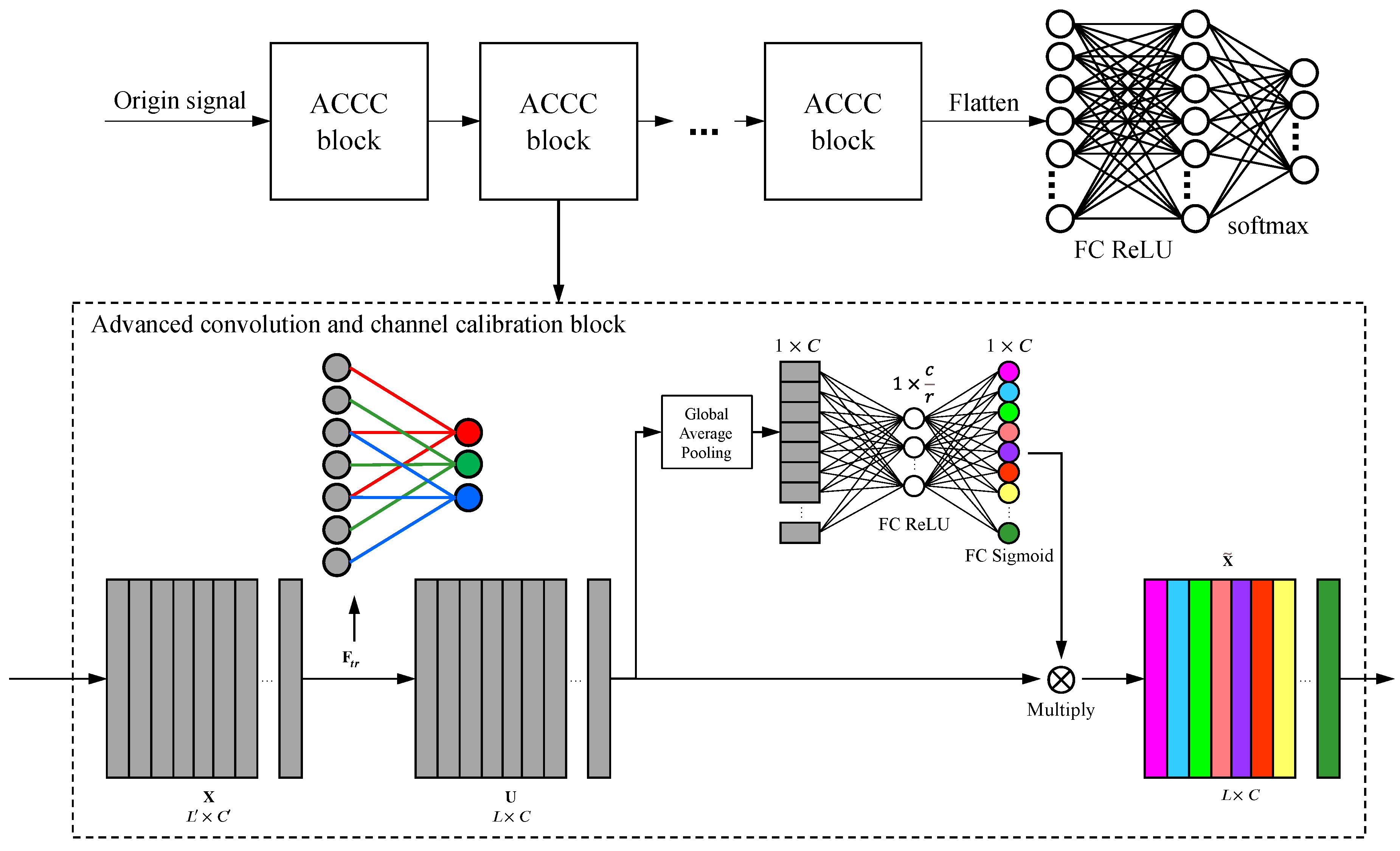
Figure 2 shows the difference between dilated convolution and standard convolution. The size of the convolution kernel of the two convolutions in the figure is 3, and stride is 1. The expansion factor is set to 1 in the extended convolution, and the expansion factor is set to 2. In Figure 2, the input signal has a length of 7, and the number of neuron receptive fields in the third layer is equal to that of the second-level convolution. The expansion convolution adopts only 6 parameters, which is 33% smaller than the normal convolution. The structure of the proposed approach is illustrated in Figure 3.

An ACCC block is a computational unit that can be built upon a transformation $F_{tr}$ mapping an input $\mathbf{X}\in {\mathbb{R}}^{L^{\prime }\times C^{\prime }}$ to feature maps $\mathbf{U}\in {\mathbb{R}}^{L\times C}$; L is the length of feature map and C is the number of filters. In the notation that $F_{tr}$ is set to be a dilated convolutional operator and $\mathbf{V}=\left[v_1,v_2,\dots ,v_c\right]$ is used to denote the learned set of filter kernels, where $v_c$ refers to the parameters of the c-th filter. Then the outputs can be written as $\mathbf{U}=[u_1,u_2,\dots ,u_c]$:

$$u_c=v_c\ast X=\sum _{s=1}^{C^{\prime }}{v}_c^s\ast x^s$$

(6)

where ∗ denotes convolution, ${\mathbf{v}}_c=\left[v_c^1,v_c^2,\dots ,v_c^{c^{\prime }}\right]$, ${\mathbf{X}}_c=\left[x_c^1,x_c^2,\dots ,x_c^{c^{\prime }}\right]$ and ${\mathbf{u}}_c\in {\mathbb{R}}^L$.

In order to obtain channel information and avoid increasing the number of model parameters, some algorithms are needed to compress the global information of the channel into a channel descriptor. Global average pooling is used in the proposed method. Formally, a statistic $z\in {\mathbb{R}}^C$ is generated by shrinking $\mathbf{U}$ through its spatial dimensions L, the c-th element of L is calculated by:

$$z_c={\mathbf{F}}_{sq}\left({\mathbf{u}}_c\right)=\frac{1}{L}\sum _{i=1}^L{u}_c\left(i\right)$$

(7)

The next step is the excitation operation, which uses the channel information obtained from the squeeze operation to capture channel dependencies. Two full connection layers are used to obtain weights. The first activation function is ReLU, and the second activation function is sigmoid. The structure can not only fully learn the dependencies between channels, but also strengthen or inhibit multiple channels. To meet these criteria, a simple gating mechanism with sigmoid activation is chosen to use:

$$s={\mathbf{F}}_{ex}(\mathbf{z},\mathbf{W})=\sigma \left(g(\mathbf{z},\mathbf{W})\right)=\sigma \left({\mathbf{W}}_2\delta \left({\mathbf{W}}_1\mathbf{z}\right)\right)$$

(8)

where $\delta$ refers to the $ReLU$ function, $W_1\in {\mathbb{R}}^{\frac{C}{r}\times C}$, and $W_2\in {\mathbb{R}}^{C\times \frac{C}{r}}$. To limit model complexity and aid generalization, the gating mechanism is parameterized by forming a bottleneck with two fully-connected (FC) layers around the non-linearity, i.e., a dimensionality-reduction layer with reduction ratio r (regarding the choice of r, it will be discussed later). A ReLU and then a dimensionality-increasing layer returning to the channel dimension of the transformation output $\mathbf{U}$. The final output of the block is obtained by rescaling $\mathbf{U}$ with the activations s:

$${\tilde{\mathbf{x}}}_c=F_{scale}\left({\mathbf{u}}_c,s_c\right)=s_c{\mathbf{u}}_c$$

(9)

where $\tilde{\mathbf{X}}=\left[{\tilde{x}}_1,{\tilde{x}}_2,\dots ,{\tilde{x}}_c\right]$ and ${\mathbf{F}}_{scale}({\mathbf{u}}_c,s_c)$ refers to channel-wise multiplication between the scalar $s_c$ and the feature map ${\mathbf{U}}_c\in {\mathbb{R}}^L$.

After stacking a certain number of ACCC blocks, ICNN is formed. This block has the following advantages:

(1)

The pooling layer of traditional convolution is replaced by the ACCC block. The number of layers required by the network is calculated according to the receptive field, and only the length of the receptive field at the last layer is approximate to that of the original signal. So the complex network design steps are eliminated.

(2)

The attentional mechanism can perform feature calibration on the feature map after dilated convolution. The key features are reinforced, and irrelevant features are suppressed. Through the accumulation of the network, key features are sifted layer by layer while irrelevant features are suppressed early.

2.5. General Procedure of the Proposed Method

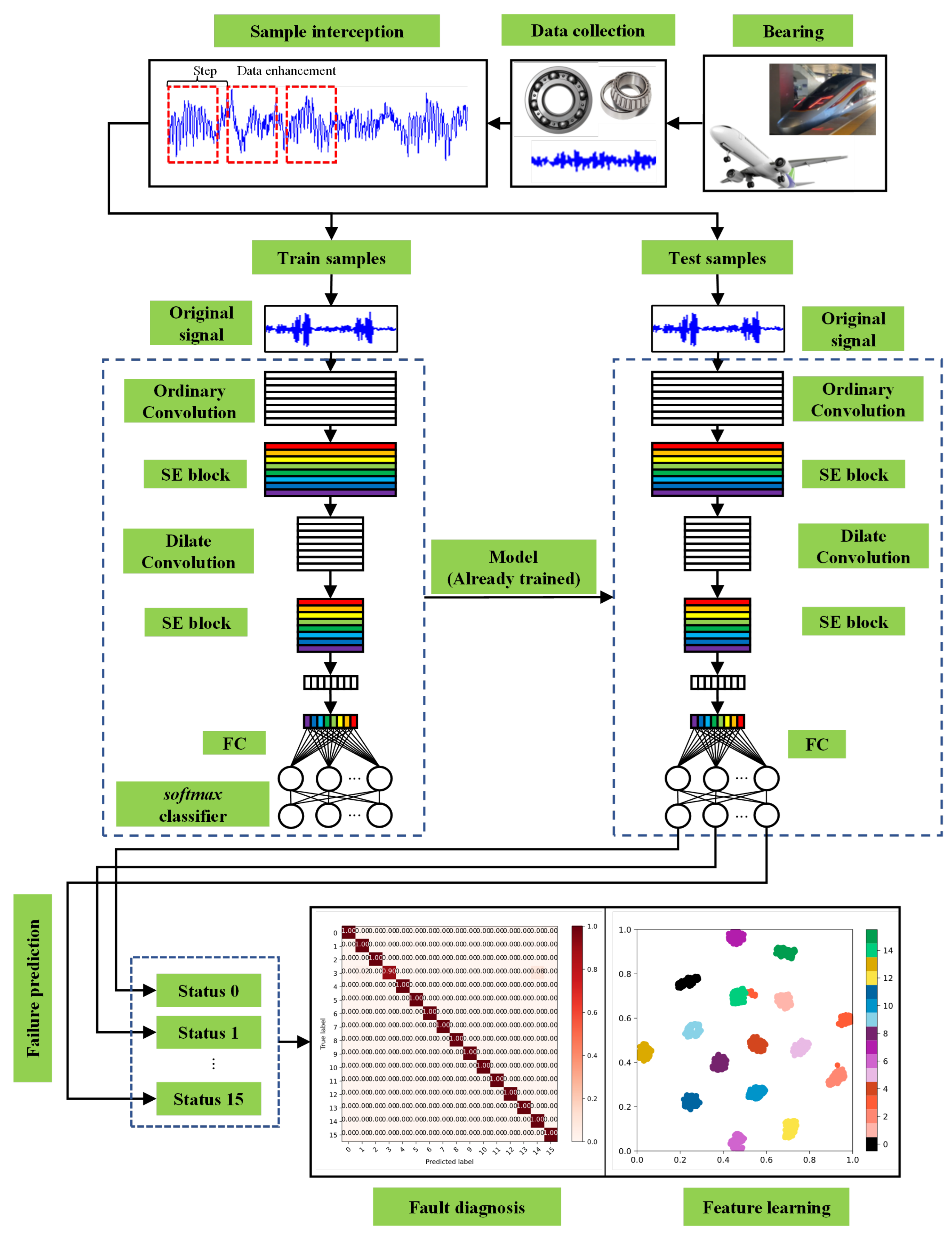
In this paper, a novel ICNN is developed for bearing fault diagnosis. The framework is shown in Figure 4. The general procedures, as shown in Figure 5, are summarized as follows:

• Step 1: Collect bearing vibration signal data.
• Step 2: The signal is divided into a training part and a test part. The next two parts use data enhancement to segment the samples. The length of each movement is the step. In this paper, the step is calculated automatically. Suppose the total length of the sample is L, the signal length of each sample is l, the number of samples is n, and the step is s. The $\left[\right]$ means rounding. The s is calculated as follows:

  $$s=\left[\frac{L-l}{n-1}\right]$$

  (10)
• Step 3: Design a neural network and input the processed data set into the network for training.
• Step 4: Use test sets or other data sets under different loads to verify the accuracy of the model.

3. Results

3.1. Validation on the CWRU Bearing Dataset

In this study, the data set comes from the bearing data set of Case Western Reserve University, shown in Figure 6, which is divided into four types of conditions: normal, ball fault, inner race fault, and outer race failure. Each type of fault can be divided into different types according to the depth of the fault or the location of the fault. There are three different load data sets, HP1, HP2, and HP3, and each of them has 16 conditions. Each condition contains 400 samples, of which 300 are train samples and 100 are test samples. Each sample is a collected vibration signal containing 1024 data points. The condition descriptions are shown in

Table 1. Description of the bearing operation conditions.

Bearing Operation Conditions	Fault Diameter	Size of Training	Label
Normal condition	-	300/100	0
Ball fault	0.007	300/100	1
Ball fault	0.014	300/100	2
Ball fault	0.021	300/100	3
Ball fault	0.028	300/100	4
Inner race fault	0.007	300/100	5
Inner race fault	0.014	300/100	6
Inner race fault	0.021	300/100	7
Inner race fault	0.028	300/100	8
Outer race fault 6 o’clock	0.007	300/100	9
Outer race fault 6 o’clock	0.014	300/100	10
Outer race fault 6 o’clock	0.021	300/100	11
Outer race fault 3 o’clock	0.007	300/100	12
Outer race fault 3 o’clock	0.021	300/100	13
Outer race fault 12 o’clock	0.007	300/100	14
Outer race fault 12 o’clock	0.021	300/100	15

.

Six traditional methods and four deep learning methods are chosen for experimentation. In the traditional methods, 15 time-domain features and 13 frequency-domain features are extracted from samples. Then BPNN and SVM are used for verification. The network structures of the four CNNs are shown in the table.

In the table, the parameters of the Conv1D function are filter number, kernel size, and dilate rate. The default value of dilate rate is 1. In the pooling layer, the pool size, and strides are both 2. The four types of CNN network structures are shown in

Table 2. Description of the structure of the four CNNS.

	1D-CNN	1D-SECNN	1D-DCNN	Improved CNN
Input Layer	(1024, 1)
Conv1D + BN layer 1	Conv1D(64, 3) (1024, 64)		Conv1D(64, 3, 2) (1020, 64)
Max Pooling1D layer 1	(512, 64)		-
Attention block layer 1	-		-
Conv1D+BN layer 2	Conv1D(64, 3) (512, 64)		Conv1D(64, 3, 4) (1012, 64)
Max Pooling1D layer 2	(256, 64)		-
Attention block layer 2	-		-
Conv1D + BN layer 3	Conv1D(64, 3) (256, 64)		Conv1D(64, 3, 8) (996, 64)
Max Pooling1D layer 3	(128, 64)		-
Attention block layer 3	-		-
Conv1D + BN layer 4	Conv1D(64, 3) (128, 64)		Conv1D(64, 3, 16) (964, 64)
Max Pooling1D layer 4	(64, 64)		-
Attention block layer 4	-		-
Conv1D + BN layer 5	Conv1D(64, 3) (64, 64)		Conv1D(64, 3, 32) (900, 64)
Max Pooling1D layer 5	(32, 64)		-
Attention block layer 5	-		-
Conv1D + BN layer 6	Conv1D(64, 3) (32, 64)		Conv1D(64, 3, 64) (772, 64)
Max Pooling1D layer 6	(16, 64)		-
Attention block layer 6	-		-
Conv1D + BN layer 7	Conv1D(64, 3) (16, 64)		Conv1D(64, 3, 128) (516, 64)
Max Pooling1D layer 7	(8, 64)		-
Attention block layer 7	-		-
Conv1D + BN layer 8	Conv1D(64, 3) (8, 64)		Conv1D(64, 3, 256) (4, 64)
Max Pooling1D layer 8	(4, 64)		-
Attention block layer 8	-		-
Flatten	(256, )
Dense	(128, )
Softmax	(16, )

.

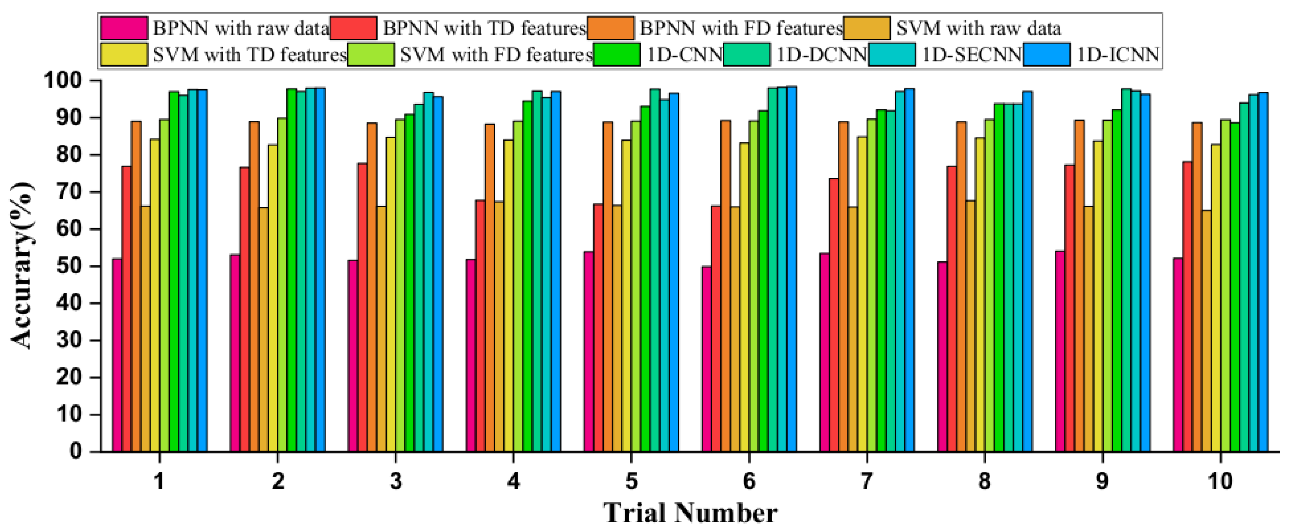
The white noise signal is added to the sample to make the SNR 0 dB. Then each method is trained 10 times to obtain the average accuracy. The average accuracy of the CNN method is much higher than BPNN and SVM with raw data, which are 52.29% and 66.25%, respectively. After feature extraction, the accuracies of BPNN and SVM increase greatly. However, their accuracy is still inferior to the proposed method. Among the four CNN networks, the traditional CNN has the lowest accuracy rate of 93.16%. Networks with dilate convolution or attention block have a certain improvement in accuracy compared to the traditional CNN. The network using these two technologies has the highest accuracy rate of 97.11%. The diagnosis results are shown in

Table 3. Diagnosis results of different methods.

Methods	Average Testing Accuracy	Standard Deviation	Correct Samples	Total Samples
BPNN with raw data	52.29%	1.32	8367	16,000
BPNN with TD features	73.78%	4.91	11,804	16,000
BPNN with FD features	88.85%	0.30	14,216	16,000
SVM with raw data	66.25%	0.76	10,600	16,000
SVM with TD features	83.85%	0.77	13,416	16,000
SVM with FD features	89.39%	0.26	14,303	16,000
1D-CNN	93.16%	2.74	14,906	16,000
1D-DCNN	95.69%	2.20	15,310	16,000
1D-SECNN	96.49%	1.46	15,438	16,000
The proposed method	97.11%	0.84	15,537	16,000

and Figure 7.

The influence of sample size on the performance of the proposed method is investigated in

Table 4. Diagnosis results based on different sizes of training samples.

Size of Training/Testing Samples	Average Testing Accuracy	Time (s)
350/50	98.87% ± 0.46%	45.08 ± 0.61
325/75	97.33% ± 0.63%	42.72 ± 0.53
300/100	97.11% ± 0.84%	39.80 ± 0.58
275/125	96.64% ± 1.44%	38.96 ± 0.67
250/150	96.49% ± 2.38%	36.33 ± 0.55
225/175	95.03% ± 3.52%	34.49 ± 0.51
200/200	90.72% ± 4.75%	30.13 ± 0.65
Avg	96.32%	38.21

.

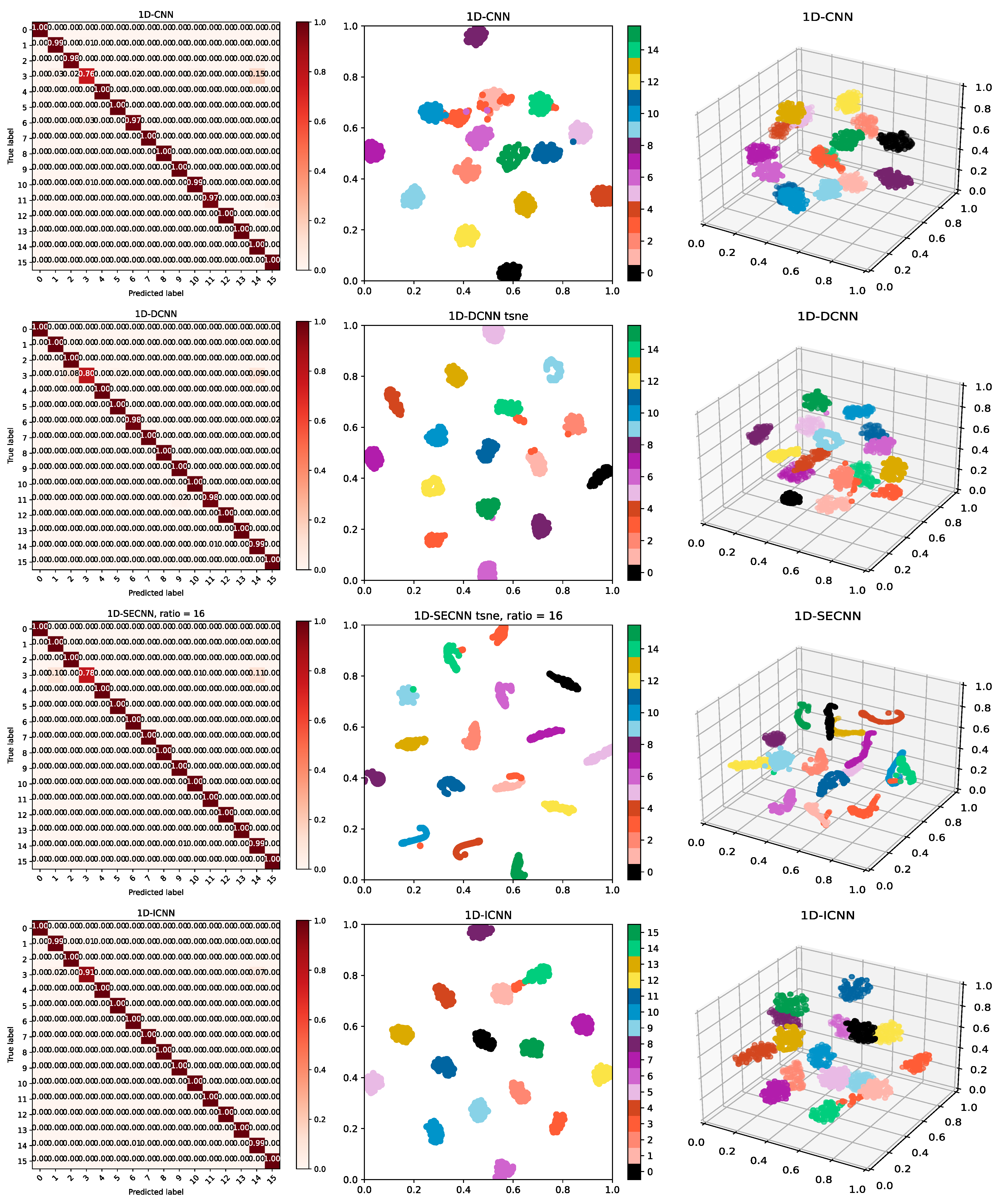
The confusion matrix and t-SNE visualization of the four CNN networks are shown in Figure 8.

From the results, the accuracy rate decreases when the percentage of training samples is relatively small. On balance, 300 is taken as the test sample and 100 is taken as the test sample.

In the ACCC block, one of the most important features is the compression ratio. Ratios of 4, 8, 16, 32, and 64 are chosen to test the accuracy. We tested CNN and SECNN, DCNN, and ICNN, respectively. We recorded the accuracy and time, and the results are shown in

Table 5. The accuracy and time under different ratios.

Model	Ratio	Accuracy	Number of Params	Time (s)
1D-CNN	-	93.16% ± 0.60% (14,906/16,000)	125,760	20.42 ± 0.78
1D-SECNN	4	95.18% ± 0.66% (15,229/16,000)	142,784	23.29 ± 1.07
	8	95.24% ± 1.77% (15,238/16,000)	134,528	21.77 ± 0.93
	16	96.49% ± 1.46% (15,438/16,000)	130,400	21.23 ± 1.24
	32	96.00% ± 0.82% (15,360/16,000)	128,336	20.82 ± 1.19
	64	95.93% ± 3.78% (15,349/16,000)	127,304	20.55 ± 0.95
	Avg	95.77%	132,670	21.53
1D-DCNN	-	95.69% ± 0.60% (15,310/16,000)	146,416	29.77 ± 0.19
The proposed method	4	96.79% ± 1.02% (15,486/16,000)	182,016	36.37 ± 0.68
	8	96.23% ± 2.88% (15,397/16,000)	172,728	36.23 ± 0.40
	16	97.11% ± 0.84% (15,537/16,000)	168,084	36.29 ± 1.22
	32	96.98% ± 1.10% (15,517/16,000)	165,762	35.56 ± 0.49
	64	96.15% ± 1.34% (15,384/16,000)	164,601	35.20 ± 0.64
	Avg	96.65%	170,638	35.93

.

It can be concluded that:

(1)

After adding the ACCC block, the accuracy rate under different compression ratios has a certain improvement compared with the traditional CNN.

(2)

In 1D-CNN, after the introduction of the ACCC block, the average time is more than one second. The accuracy rate is increased by more than 2%, and the effect is very satisfactory. In 1D-DCNN, after introducing the ACCC block, it took six seconds longer and the accuracy rate increased by nearly 1% and still has good results. It is worthwhile to increase the training time slightly in exchange for accuracy.

Therefore, considering the accuracy and time factors, the ratio is chosen as 16 for the next experiment.

In this experiment, the samples are added with different intensities of noise. The above 10 methods are used to train separately. The accuracies they obtained are shown in

Table 6. The accuracy of each method under different SNRs.

Method	SNR (dB)
	3	2	1	0	−1	−2	−3	−4	Avg
1D-CNN	95.25%	94.13%	91.94%	91.12%	90.44%	89.56%	78.62%	74.94%	88.25%
1D-DCNN	97.37%	97.06%	96.81%	93.62%	93.25%	91.31%	89.50%	83.00%	92.74%
1D-SECNN	98.37%	98.31%	97.94%	94.94%	94.81%	89.81%	85.87%	81.19%	92.66%
The proposed method	98.00%	97.62%	97.12%	96.56%	95.81%	94.69%	93.31%	85.12%	94.78%

and Figure 9.

It can be concluded that traditional methods need to manually extract features, otherwise the accuracy rate will be very low. However, the CNN does not need to manually extract features, only input the original signal. In any case, the accuracy of the traditional method is not comparable to that of the CNN. Compared with the traditional CNN, dilated convolution and attention block can improve the accuracy to a certain extent. The proposed method is inferior to 1D-SECNN when the SNR is over zero, but it achieves the highest accuracy in a high-noise environment. This may indicate that the proposed method has strong anti-interference ability and domain adaptability.

3.2. Validation on the NASA Bearing Dataset

In this section, the NASA bearing data set is used to further demonstrate the superiority of the proposed method. Data from day 25 to 35 of bearing No. 3 in data set No. 1 are extracted for the experiment. A total of 9600 training samples and 9600 test samples are collected. Three kinds of bearing operation conditions are created, which are in health condition, slight degradation condition, and severe degradation condition. The sample length is 1024. The data set description is shown in

Table 7. NASA data set description.

Conditions	Days	Train Samples	Test Samples	Label
Health	25–30	4800	4800	0
Slight degradation	30–32	1920	1920	1
Severe degradation	32–35	2880	2880	2

.

The ten methods mentioned above have been tested, and the results are shown in

Table 8. Diagnosis results for the NASA bearing data set.

Methods	Average Testing Accuracy	Standard Deviation	Average Training Time (s)
BPNN with raw data	40.93%	1.89	18.2
BPNN with TD features	50.68%	0.56	17.2
BPNN with FD features	68.26%	0.49	17.5
SVM with raw data	45.93%	1.78	11.1
SVM with TD features	55.35%	0.44	10.6
SVM with FD features	72.38%	0.31	10.8
1D-CNN	82.56%	0.92	30.5
1D-DCNN	86.38%	1.19	40.3
1D-SECNN	86.79%	1.23	33.6
The proposed method	90.26%	1.36	42.5

.

Experimental results show that although the training time of the proposed method is slightly increased compared with other methods, it can more accurately distinguish the life cycle stages of bearings.

4. Conclusions

In this paper, a new ICNN for bearing fault diagnosis is proposed. The network can not only retain the timing relation of the original signal to the maximum extent, but also strengthen the important features and suppress the irrelevant features. The proposed algorithm is validated on two data sets. The results show that the proposed algorithm achieves the highest average accuracy, which is better than traditional methods and ordinary deep learning methods.

References

1. Zhang, B.; Zhang, S.; Li, W. Bearing performance degradation assessment using long short-term memory recurrent network. Comput. Ind. 2019, 106, 14–29. [Google Scholar] [CrossRef]
2. Gao, Z.; Cecati, C.; Ding, S.X. A survey of fault diagnosis and fault-tolerant techniques—Part I: Fault diagnosis with model-based and signal-based approaches. IEEE Trans. Ind. Electron. 2015, 62, 3757–3767. [Google Scholar] [CrossRef] [Green Version]
3. Zhiwei, G.; Cecati, C.; Ding, S.X. A survey of fault diagnosis and fault-tolerant techniques—Part II: Fault diagnosis with knowledge-based and hybrid/active approaches. IEEE Trans. Ind. Electron. 2015, 62, 3768–3774. [Google Scholar]
4. LeCun, Y.; Bengio, Y.; Hinton, G. Deep learning. Nature 2015, 521, 436–444. [Google Scholar] [CrossRef] [PubMed]
5. Schmidhuber, J. Deep learning in neural networks: An overview. Neural Netw. 2015, 61, 85–117. [Google Scholar] [CrossRef] [Green Version]
6. Shao, H.; Jiang, H.; Zhang, H.; Liang, T. Electric locomotive bearing fault diagnosis using a novel convolutional deep belief network. IEEE Trans. Ind. Electron. 2017, 65, 2727–2736. [Google Scholar] [CrossRef]
7. Shao, H.; Jiang, H.; Wang, F.; Zhao, H. An enhancement deep feature fusion method for rotating machinery fault diagnosis. Knowl.-Based Syst. 2017, 119, 200–220. [Google Scholar] [CrossRef]
8. AlThobiani, F.; Ball, A.; Tran, V.T. An approach to fault diagnosis of reciprocating compressor valves using Teager–Kaiser energy operator and deep belief networks. Expert Syst. Appl. 2014, 41, 4113–4122. [Google Scholar]
9. Janssens, O.; Slavkovikj, V.; Vervisch, B.; Stockman, K.; Loccufier, M.; Verstockt, S.; Van de Walle, R.; Van Hoecke, S. Convolutional neural network based fault detection for rotating machinery. J. Sound Vib. 2016, 377, 331–345. [Google Scholar] [CrossRef]
10. Dhiman, G.; Juneja, S.; Viriyasitavat, W.; Mohafez, H.; Hadizadeh, M.; Islam, M.A.; El Bayoumy, I.; Gulati, K. A Novel Machine-Learning-Based Hybrid CNN Model for Tumor Identification in Medical Image Processing. Sustainability 2022, 14, 1447. [Google Scholar] [CrossRef]
11. Shao, S.; McAleer, S.; Yan, R.; Baldi, P. Highly accurate machine fault diagnosis using deep transfer learning. IEEE Trans. Ind. Inform. 2018, 15, 2446–2455. [Google Scholar] [CrossRef]
12. Krizhevsky, A.; Sutskever, I.; Hinton, G.E. Imagenet classification with deep convolutional neural networks. In Advances in Neural Information Processing Systems 25 (NIPS 2012); Association for Computing Machinery: New York, NY, USA, 2017. [Google Scholar]
13. Wen, L.; Li, X.; Gao, L.; Zhang, Y. A new convolutional neural network-based data-driven fault diagnosis method. IEEE Trans. Ind. Electron. 2017, 65, 5990–5998. [Google Scholar] [CrossRef]
14. Zhao, J.; Yang, S.; Li, Q.; Liu, Y.; Gu, X.; Liu, W. A new bearing fault diagnosis method based on signal-to-image mapping and convolutional neural network. Measurement 2021, 176, 109088. [Google Scholar] [CrossRef]
15. Gong, W.; Wang, Y.; Zhang, M.; Mihankhah, E.; Chen, H.; Wang, D. A Fast Anomaly Diagnosis Approach Based on Modified CNN and Multisensor Data Fusion. IEEE Trans. Ind. Electron. 2022, 69, 13636–13646. [Google Scholar] [CrossRef]
16. Huang, D.; Li, S.; Qin, N.; Zhang, Y. Fault diagnosis of high-speed train bogie based on the improved-CEEMDAN and 1-D CNN algorithms. IEEE Trans. Instrum. Meas. 2021, 70, 3508811. [Google Scholar] [CrossRef]
17. Peng, D.; Wang, H.; Liu, Z.; Zhang, W.; Zuo, M.J.; Chen, J. Multibranch and multiscale CNN for fault diagnosis of wheelset bearings under strong noise and variable load condition. IEEE Trans. Ind. Inform. 2020, 16, 4949–4960. [Google Scholar] [CrossRef]
18. Xiong, J.; Li, C.; Wang, C.D.; Cen, J.; Wang, Q.; Wang, S. Application of Convolutional Neural Network and Data Preprocessing by Mutual Dimensionless and Similar Gram Matrix in Fault Diagnosis. IEEE Trans. Ind. Inform. 2021, 18, 1061–1071. [Google Scholar] [CrossRef]
19. Mo, Z.; Zhang, Z.; Tsui, K.L. The variational kernel-based 1-D convolutional neural network for machinery fault diagnosis. IEEE Trans. Instrum. Meas. 2021, 70, 3523210. [Google Scholar] [CrossRef]
20. Zhang, D.; Chen, Y.; Guo, F.; Karimi, H.R.; Dong, H.; Xuan, Q. A new interpretable learning method for fault diagnosis of rolling bearings. IEEE Trans. Instrum. Meas. 2020, 70, 3507010. [Google Scholar] [CrossRef]
21. Chen, J.; Huang, R.; Zhao, K.; Wang, W.; Liu, L.; Li, W. Multiscale convolutional neural network with feature alignment for bearing fault diagnosis. IEEE Trans. Instrum. Meas. 2021, 70, 3517010. [Google Scholar] [CrossRef]
22. Yu, J.; Zhou, X. One-dimensional residual convolutional autoencoder based feature learning for gearbox fault diagnosis. IEEE Trans. Ind. Inform. 2020, 16, 6347–6358. [Google Scholar] [CrossRef]
23. Shao, H.; Xia, M.; Han, G.; Zhang, Y.; Wan, J. Intelligent fault diagnosis of rotor-bearing system under varying working conditions with modified transfer convolutional neural network and thermal images. IEEE Trans. Ind. Inform. 2020, 17, 3488–3496. [Google Scholar] [CrossRef]
24. Li, G.; Wu, J.; Deng, C.; Chen, Z.; Shao, X. Convolutional neural network-based Bayesian Gaussian mixture for intelligent fault diagnosis of rotating machinery. IEEE Trans. Instrum. Meas. 2021, 70, 3517410. [Google Scholar] [CrossRef]
25. Guo, S.; Zhang, B.; Yang, T.; Lyu, D.; Gao, W. Multitask convolutional neural network with information fusion for bearing fault diagnosis and localization. IEEE Trans. Ind. Electron. 2019, 67, 8005–8015. [Google Scholar] [CrossRef]
26. Xie, T.; Huang, X.; Choi, S.K. Intelligent Mechanical Fault Diagnosis Using Multisensor Fusion and Convolution Neural Network. IEEE Trans. Ind. Inform. 2021, 18, 3213–3223. [Google Scholar] [CrossRef]
27. Hu, J.; Shen, L.; Sun, G. Squeeze-and-excitation networks. In Proceedings of the IEEE Conference on Computer Vision and Pattern Recognition, Salt Lake City, UT, USA, 18–22 June 2018; pp. 7132–7141. [Google Scholar]
28. Gao, Z.; Xie, J.; Wang, Q.; Li, P. Global second-order pooling convolutional networks. In Proceedings of the IEEE/CVF Conference on Computer Vision and Pattern Recognition, Long Beach, CA, USA, 15–20 June 2019; pp. 3024–3033. [Google Scholar]
29. Fu, J.; Liu, J.; Tian, H.; Li, Y.; Bao, Y.; Fang, Z.; Lu, H. Dual attention network for scene segmentation. In Proceedings of the IEEE/CVF Conference on Computer Vision and Pattern Recognition, Long Beach, CA, USA, 15–20 June 2019; pp. 3146–3154. [Google Scholar]
30. Chen, Z.; Gryllias, K.; Li, W. Intelligent fault diagnosis for rotary machinery using transferable convolutional neural network. IEEE Trans. Ind. Inform. 2019, 16, 339–349. [Google Scholar] [CrossRef]
31. Wang, H.; Liu, Z.; Peng, D.; Yang, M.; Qin, Y. Feature-level attention-guided multitask CNN for fault diagnosis and working conditions identification of rolling bearing. IEEE Trans. Neural Netw. Learn. Syst. 2021, 33, 4757–4769. [Google Scholar] [CrossRef]
32. Fang, H.; Deng, J.; Zhao, B.; Shi, Y.; Zhou, J.; Shao, S. LEFE-Net: A lightweight efficient feature extraction network with strong robustness for bearing fault diagnosis. IEEE Trans. Instrum. Meas. 2021, 70, 3513311. [Google Scholar] [CrossRef]
33. Wang, H.; Xu, J.; Yan, R.; Gao, R.X. A new intelligent bearing fault diagnosis method using SDP representation and SE-CNN. IEEE Trans. Instrum. Meas. 2019, 69, 2377–2389. [Google Scholar] [CrossRef]
34. Zhou, Y.; Li, J.; Chi, J.; Tang, W.; Zheng, Y. Set-CNN: A text convolutional neural network based on semantic extension for short text classification. Knowl.-Based Syst. 2022, 257, 109948. [Google Scholar] [CrossRef]
35. Song, Z.; Zhao, X.; Hui, Y.; Jiang, H. Fusing Attention Network based on Dilated Convolution for Super Resolution. IEEE Trans. Cogn. Dev. Syst. 2022, 15, 234–241. [Google Scholar] [CrossRef]
Figure 1. Structure of the convolutional neural network.
Actuators 12 00154 g001
Figure 2. Standard convolution layer (a) and dilated convolution layer (b).
Actuators 12 00154 g002
Figure 3. The ICNN model structure.
Actuators 12 00154 g003
Figure 4. Proposed method for a fault diagnosis framework.
Actuators 12 00154 g004
Figure 5. The flowchart of the proposed method.
Actuators 12 00154 g005
Figure 6. CWRU rolling bearing data acquisition system.
Actuators 12 00154 g006
Figure 7. Diagnosis results of the ten trials using different methods.
Actuators 12 00154 g007
Figure 8. Confusion matrix of four types of networks: 2D and 3D t-SNE visualization.
Actuators 12 00154 g008
Figure 9. Accuracy image of each method under different SNRs.
Actuators 12 00154 g009