
Kinematic Analysis of a New 3-DOF Parallel Wrist-Gripper Assembly with a Large Singularity-Free Workspace

Department of Mechanical Engineering, Université Laval, Québec, QC G1V 0A6, Canada
*
Author to whom correspondence should be addressed.
†
These authors contributed equally to this work.
Actuators 2023, 12(11), 421; https://doi.org/10.3390/act12110421
Submission received: 21 September 2023
/
Revised: 25 October 2023
/
Accepted: 2 November 2023
/
Published: 10 November 2023
(This article belongs to the Special Issue Advancement in the Design and Control of Robotic Grippers)
Abstract
:This paper introduces a novel dexterous 3-DOF parallel wrist-gripper assembly with a large singularity-free range of motion. It consists of a zero-torsion 2-DOF parallel wrist and a 1-DOF parallel gripper. The wrist produces a 2-DOF sphere-on-sphere pure rolling motion. This large singularity-free 2-DOF sphere-on-sphere pure rolling motion of the wrist allows for smooth and precise manipulation of objects in various orientations, making it suitable for applications such as assembly, pick-and-place, and inspection tasks. Using a geometrical approach, analytical solutions for the inverse and forward kinematics problems of the wrist and gripper are derived. From the inverse kinematic equations, the Jacobian matrices are derived and it is shown that the whole workspace is free of type I and type II singularities. It is shown that with a proper choice of design variables, a large singularity-free range of motion can be obtained. The absence of singularities in the whole workspace of the wrist-gripper assembly is an important feature that enhances its reliability. Finally, the correctness of the derived equations for the wrist inverse and forward kinematics are verified using MSC Adams. These results confirm the feasibility and effectiveness of the proposed parallel wrist-gripper assembly. Overall, the novel parallel wrist-gripper assembly presented in this paper demonstrates great potential for improving the efficiency and flexibility of robotic manipulators in a variety of industrial and research applications.
1. Introduction
The field of parallel manipulators (PMs) has seen significant growth in recent years due to their numerous advantages over traditional serial robots, such as higher stiffness, speed, precision, and load to weight ratio. However, PMs also have some disadvantages, including a smaller workspace, more singular configurations, and more complex kinematics [1,2]. Recent research initiatives are proposing means of alleviating these drawbacks, such as, for instance, the use of kinematic redundancy [3].
One area of focus within PM research has been the development of wrist designs. Advances in this area include the proposal of a spherical parallel manipulator (SPM) with three rotational degrees of freedom, which led to the design of the Agile Eye and later the Agile Wrist [4,5]. Recently, a comprehensive review of 3-DOF rotational parallel mechanisms was conducted [6]. A number of 2-DOF spherical parallel manipulators (SPMs) have been patented and developed, each with their own unique design and capabilities. In reference [7], a 2-DOF SPM was patented using a five-bar structure. Ueda introduced an SPM based on a six-bar linkage with a yaw and – pitch range [8]. Duan et al. designed a 2-DOF SPM with a U-2RRR architecture and analyzed its kinematic and dynamic behaviour [9]. Cammarata created a U-2PUS 2-DOF SPM that can achieve a singularity-free tilt angle [10]. Carricato and Parenti-Castelli introduced a fully decoupled 2-DOF parallel wrist that can independently actuate each Euler angle [11]. Bajaj et al. conducted a recent review of other 2-DOF SPMs [12].
At the core of all of these 2-DOF SPMs lies a fundamental concept—the fixed centre of rotation (FCOR) around which they all rotate, and the continuous alignment of the instantaneous screw axis (ISA) with this central point—irrespective of their configurations.
In a recent breakthrough, a pioneering approach has emerged to unlock the potential of 2-DOF rotational parallel manipulators (RPMs) within a significantly expanded and singularity-free workspace. Leading works by Sofka et al. [13], Dong et al. [14], Wu et al. [15], Shah et al. [16], and Chang et al. [17] have championed this concept.
In this groundbreaking paradigm, the conventional fixed centre of rotation becomes a dynamic element, residing on a sphere throughout various configurations. Importantly, the ISA now passes through this non-fixed centre of rotation. It was Dunlop and Jones who initially harnessed this innovative idea to craft the Canterbury tracker for solar tracking [18].
Expanding on this notion, Rosheim and Sauter designed the Omni-Wrist III, a remarkable 4-4R RPM that boasts a hemisphere-like workspace devoid of singularities [19].
Wu et al. [20] introduced the term ’equal spherical pure rotations’ (ESPR) to describe this form of rotation. They adopted a graphical approach proposed by Yu et al. [21] to deduce the freedom and complementary constraint patterns (FCCPs) inherent in robots with ESPR characteristics. Their classification system identified three distinct types of these mechanisms.
Subsequently, Yu et al. ventured further into the field, analyzing a set of n-4R RPMs. Their investigations shed light on the relationship between n and the degrees of freedom available in these mechanisms [22].
Adding a 1-DOF grasping ability to wrists is another emerging topic in PMs [23]. Although 3-DOF and 2-DOF wrists have received considerable attention, the topic of 3-DOF and 4-DOF wrist-grippers has remained largely unexplored. Most of the work performed in this area is regarding using the wrist-gripper mechanism for minimally invasive surgery (MIS). Some researchers introduced tendon-driven mechanisms [24,25], and some researchers used linkage-based designs [26,27]. Yamashita et al. [28] introduced a 3-DOF endoscopic handheld forceps manipulator for use in endoscopic surgery. They utilized a multi-slider linkage to transform linear motion of linkages to rotation of frames, enabling 2-DOFs of rotational motion. Also, a 1-DOF wire-driven gripper is added to the wrist to complete the wrist-gripper assembly. Hong and Jo proposed a 4-DOF parallel wrist-gripper mechanism. In this mechanism, the end-effector of the wrist is connected to the base via legs and central leg. The architecture, creates two rotational DOFs and one translational DOF. By adding one leg to the mechanism, the translational DOF is converted to a grasping motion by the inversion of the slider–crank linkage. Also, the axial rotation of the central leg produces a pure axial rotation for the gripper [29]. Bazman et al. [30] proposed a 4-DOF wrist-gripper mechanism with a - architecture. In this mechanism the end-effector can undergo a pitch–yaw rotation and a thrust motion using a parallel mechanism. The central leg is used to convert the thrust motion into a grasping motion by the inversion of the slider–crank linkage. Also, a rotary actuator in series is added to the base to provide the roll axis motion. Sanchez et al. [31] introduced a surgical instrument featuring a universal wrist that uses a —S configuration. The instrument shaft is connected to a ball joint on the central link, which in turn is seated in the base of the end-effector. The other three PS linkages are manipulated to produce both pitch and yaw motions in a redundant manner. This redundancy arises because the linkage connected to the movable jaw serves a dual purpose: it is used both to open and close the gripper and to actuate the end-effector’s rotational motion. Ghaedrahmati and Gosselin [32] proposed a novel parallel —, 1 leg architecture. This architecture enables the mechanism to rotate on a full hemisphere without encountering singularity, making it highly suitable as either a 2-DOF or 3-DOF wrist gripper with minor modifications. The proposed mechanism’s unique design allows for greater flexibility and precision in various industrial applications, such as robotic assembly and manufacturing.
This paper presents a novel and dexterous wrist-gripper assembly with a large singularity-free workspace, consisting of a 2-DOF equal spherical pure rotation (ESPR) wrist and a 1-DOF gripper. The ESPR wrist is a zero-torsion RPM [33] and offers 2-DOFs, pure azimuth and tilt angle, which enables the mechanism to attain a wide range of orientations and reachability in confined spaces. The addition of the 1-DOF gripper further enhances the mechanism’s capabilities, providing the grasping ability required to manipulate various objects. The proposed mechanism is lightweight and fast, making it suitable for a variety of applications in fields such as robotics, manufacturing, and biomedical engineering. With its high dexterity and large workspace, the mechanism is able to perform complex tasks such as object manipulation, assembly, and inspection with ease. The presented mechanism offers an efficient and effective solution to the challenges posed by confined spaces and complex tasks. Moreover, another advantage of the proposed architecture is that no actuator is required at the end-effector to operate the gripper, which reduces the mass and inertia of the end-effector and eliminates the need for electronics at the end-effector. This feature facilitates washing and disinfection operations for applications where those are needed.
The organization of this paper is as follows. In Section 2, the robot architecture is described. In Section 3, the kinematic model of the wrist and gripper is developed. Specifically, Section 3.1 presents the inverse kinematic model of the wrist, while Section 3.2 develops the forward kinematic model of the wrist and provides analytical solutions for the forward kinematic problem. Section 3.3 and Section 3.4 then provide the inverse kinematic and forward kinematic of the gripper, respectively. The Jacobian matrices of the wrist are derived using two methods in Section 3.5 and Section 3.6. Section 4 offers a comprehensive analysis of wrist singularities, focusing on the derivation of specific geometric conditions that lead to singularity occurrences. In Section 5, the rotational and translational workspace of the end-effector is explored in detail, providing a comprehensive representation of workspace characteristics. Section 6.1 and Section 6.2 present the results of a simulation study conducted using MSC Adams to validate the derived equations for inverse and forward kinematics. The verification of these models is thoroughly discussed. Section 7 offers a thorough comparative analysis against the current state of the art. Finally, Section 8 concludes the paper with some remarks.
2. Robot Architecture
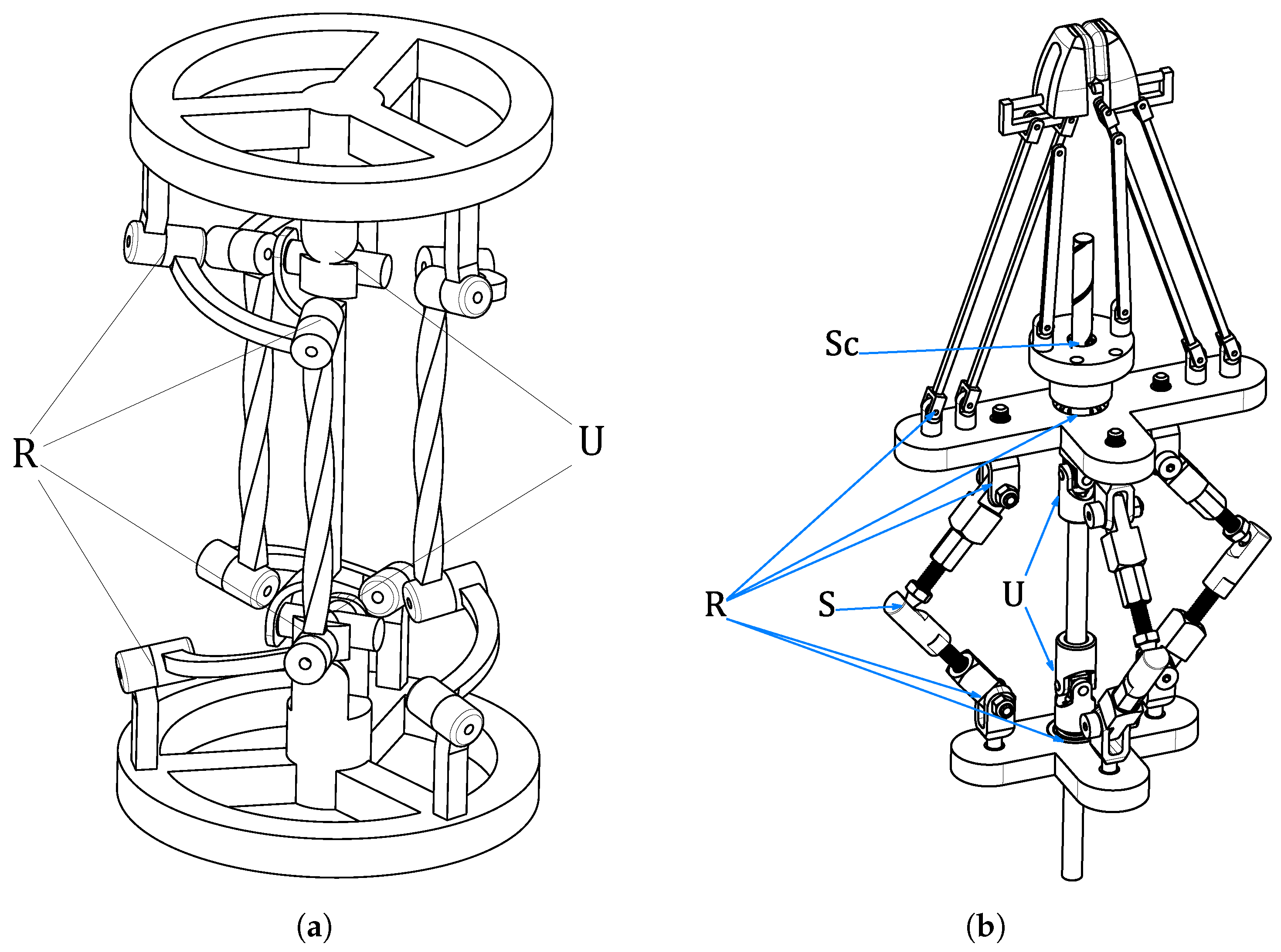
The proposed mechanism is a spatial wrist-gripper parallel robot. As can be seen from Figure 1, the end-effector of the wrist is connected to the base via — legs and one leg. Here, , R, S, and U stand for an active revolute joint, a passive revolute joint, a passive spherical joint, and a passive universal joint, respectively. Also, the rotational output of the leg is used as the motion input of the lead screw to open and close the gripper. Globally, the assembly is a 3-DOF mechanism, consisting of a 2-DOF equal spherical pure rotations (ESPRs) wrist and a 1-DOF gripper. The rotational motion of the wrist is completely decoupled from the opening motion of the gripper. Three motors can be mounted on the base in order to actuate the mechanism. The two motors that actuate the base R joints of the wrist can be mounted either to actuate the first and second legs or the first and third legs, and the third motor actuates the shaft that is connected to the base via a revolute joint. The revolute joints and the universal joint that are connected to the base must be co-planar.
As can be seen from Figure 2a, in each leg vector, is the vector from the centre of the first universal joint to the centre of the first revolute joint, is the vector from the centre of the first revolute joint to the centre of the first spherical joint, is the vector from the centre of the first spherical joint to the centre of the second revolute joint, and is the vector from the centre of the second universal joint to the centre of the second revolute joint. The plane of symmetry is a plane that passes through the midpoint A of the UU leg and the three spherical joints and is perpendicular to vector , where is the vector from O to . Actuator joint coordinates are denoted for the 2-DOF wrist and for the gripper. In each leg, vectors and are symmetric to vectors and , respectively, with respect to the plane of symmetry .
3. Kinematic Modelling
3.1. Inverse Kinematics Modelling (Wrist)
First, the reflection matrix associated with the plane of symmetry is defined using the unit vector defined in the direction of vector . One has
In order to derive the end-effector rotation matrix , a moving coordinate system is attached to the end-effector. The following relations between moving coordinate unit vectors and fixed coordinate unit vectors can be written:
where , , and are the columns of the reflection matrix . Using the unit vectors of Equation (2), the following expression can be derived for :
By comparing Equations (1) and (3), the following relation can be found between the end-effector rotation matrix and the reflection matrix :
in which .
In the inverse kinematics problem, it is assumed that the end-effector tilt and azimuth angles are known, and the purpose is to find the actuator angles . In [32], it was shown that the tilt angle of the end-effector in a wrist with the ESPR rotational property is twice the tilt angle of the UU leg and the azimuth angles are equal (Figure 2b). Hence, by knowing the end-effector tilt angle () and azimuth angle (), the unit vector along the UU leg will have a tilt angle () and azimuth angle (). So, is defined as
By knowing the unit vector , the reflection matrix can be derived using Equation (1). Then, the end-effector rotation matrix can be found using Equation (4b). From Figure 2a the following relation can be written:
Also, from Figure 2a the following equations can be written:
where corresponds to vector expressed in the end-effector frame. By substituting Equation (7) into Equation (6), one can obtain:
Also, using the fact that , and using Equation (4), one obtains
and the simplification of Equation (9) leads to
where the fact that was used. Then, using Equation (1), and using , leads to
From Equation (11), the following equation can be inferred:
Equation (12) can be rewritten as follows:
By expansion of Equation (13), the solution for the inverse kinematics can be derived as follows:
where b is the distance from the intermediate U joint to the revolute joint at the base of each of the RSR legs and l is the length of the links connecting the base R joints to the intermediate S joints in each leg. Using the definition of the tangent of the half of the angle (i = 1, 2), namely, , Equation (14) can be written as
in which
Assuming , , and by substituting , , and from Equation (5), the coefficients can be expanded as follows:
and can be found as
which concludes the solution of the inverse kinematic problem. It can be observed that two solutions exist for each of the legs. Equation (18) holds if . This fact will be discussed further in Section 5.
3.2. Forward Kinematic Modelling (Wrist)
Solving the forward kinematic problem for this robot is a relatively straightforward task. In this context, we begin with the assumption that the joint angles (where ) are known, and the objective is to determine the tilt and twist angles of the UU leg, represented by the vector . To achieve this, we expand Equation (12) by utilizing the vectors , , and . This expansion results in the following:
Using the definition of the tangent of half of the angles and , Equation (19) can be written as
in which
Assuming as a hidden variable, Equation (20) can be written as
in which
The Sylvester matrix [34] that is associated with the two univariate polynomials in Equations (21a) and (21b) can be written as
The determinant of matrix must be zero for the equations to have a common root, namely,
Equation (23) leads to a polynomial of degree six as follows:
in which
One solution of Equation (24) is
this value corresponds to and gives the coefficients of Equation (21) as follows:
Importantly, this situation () corresponds to the initial position, where . Consequently, , making Equation (21a) zero. However, it is worth noting that when (or equivalently, ), the angle , and correspondingly , become undefined. This is because is defined as the angle between the projection of d on the xy plane and the x-axis. In the () scenario, the projection collapses to a point, rendering the angle meaningless.
Four non-trivial solutions of Equation (21) can be calculated using the following change in the variable , which yields:
The solution of Equation (26) can be written as:
As can be seen from Equation (26), exists if and only if . The expansion of this term is as follows:
is satisfied if and only if
By iteratively adjusting the coefficients and , one can determine values that satisfy Equation (29) within the range of . This will be discussed further in Section 5.
Then, four solutions for can be calculated as:
As is evident from Equation (30), to obtain real solutions for , it is imperative that be a non-negative value. This critical condition will be further explored in Section 5. Hence, one can obtain the tilt angle as follows:
When the solution for is known, it can be substituted into Equation (19) and the solutions for and can be derived as
Then, angle can be found as follows:
which yields a maximum of four solutions for angle .
3.3. Inverse Kinematic Modelling (Gripper)
In the inverse kinematics problem of the gripper, is known, and the purpose is to find , where, as shown in Figure 3, is the opening of the gripper and is the displacement of the input lead screw. Once is determined, the input angle can be calculated using the pitch of the lead screw.
From Figure 3, the following relations can be written:
where the angles and lengths are as defined in Figure 3. From Equation (34a), the following relation can be found for :
so,
also from Equations (34b) and (34c), and using Equations (35) and (36), and can be found as follows:
On the other hand, one can write
Substituting (37a) and (37b) into (38), one can obtain two quadratic equations in (because there are two answers for ). The solution of these two quadratic equations leads to four solutions for as a function of . Using the fact that the central leg is a double Cardan joint, the input angle can be related to the displacement and the lead screw thread pitch p as follows:
where is the input angle in degrees, as shown in Figure 2a.
3.4. Forward Kinematic Modelling (Gripper)
In the forward kinematics problem, it is assumed that is known, and the purpose is to find . First, from Equation (39), can be derived, then from Equations (34b) and (34c), the following relation can be found for and :
Substituting Equation (40) into Equation (38) and using the definition of the tangent of half of the angle leads to a quadratic equation in . Solving this equation leads to two solutions for , which then leads to two solutions for as a function of :
when is known, using Equation (34a), can be found as a function of , and subsequently as a function of the input angle .
3.5. Wrist Jacobian Matrices (Method I)
The time derivative of Equation (12) leads to
Also, by definition, , hence the time derivative of leads to
in which
Also, the time derivative of vector leads to
in which and is
By substituting Equations (43) and (45) into Equation (42), one can obtain
Using Equation (46), Equation (47) can be rewritten as follows:
in which . From Equation (48), the Jacobian matrices can be derived as follows:
3.6. Wrist Jacobian Matrices (Method II)
The Jacobian matrices can be derived using another method. The time derivative of Equation (4b) leads to
and the end-effector angular velocity can be found as follows:
By substituting Equation (4a), into Equation (51) and using the fact that the reflection matrix is a symmetric matrix, i.e., , one can obtain
and also , in which is the identity matrix. Hence,
Also, from Equation (1), one can multiply both sides of the equation by to obtain
and from the fact that , Equation (54) yields
The time derivative of Equation (55) leads to
and using Equation (1), Equation (56) leads to
Using the definition of vector and Equation (45), it can be found that . Hence, Equation (57) leads to
and by substituting Equation (55) into Equation (58), one can obtain:
which, using Equation (53), can be written as
in which is the angular velocity of the end-effector. Substituting Equations (43) and (60) into Equation (42) leads to
and the Jacobian matrices can be derived from Equation (61) as follows:
in which is a matrix. The end-effector angular velocity matrix can be derived using Equation (53) as follows:
The end-effector angular velocity can be derived using Equation (63) as follows:
and then, the end-effector angular velocity can be written as follows:
in which
Matrix can be rewritten using vector components and from matrix , which is defined in Equation (46) as follows:
Substituting Equation (67) into Equation (65) and then into Equation (61) leads to
The expansion of Equation (68) yields
Also, from the definition of vectors , , and one can obtain
Substituting Equation (70) into Equation (69) leads to
which is the same equation as Equation (48).
4. Singularity Analysis (Wrist)
The workspace of parallel robots is limited by the presence of singularities, which can be classified into two types: type I and type II. While scaling can increase the translational workspace, it has no effect on the rotational workspace.
A type I singularity corresponds to a singularity of matrix in Equation (49), that is, when . In this mechanism, this type of singularity occurs when vectors and (i = 1, 2) become perpendicular.
A type II singularity is associated with a singularity in matrix J as defined in Equation (49). Such a singularity arises when . The calculation of the determinant of matrix J is outlined as follows:
in which . From the definition of and in Equation (46), matrix can be derived as follows:
It can be observed from Equation (73) that matrix is skew-symmetric; therefore, Equation (72) can be rewritten as follows:
where . Hence, Equation (74) can be rewritten as
According to Equation (75), it is evident that the determinant becomes zero when vectors n, , and align in a co-planar configuration or when . In such scenarios, a type II singularity is encountered. The examination of the mathematical conditions for these singular points will be a central focus of the workspace analysis, with the objective of ascertaining the presence of singularities within the workspace.
5. Workspace Analysis (Wrist)
The wrist rotational workspace can be found using the inverse kinematics solution derived in Equation (18). In fact, it can be said that the rotational workspace is the domain of Equation (18). A set of is in the domain of Equation (18) if it satisfies the following conditions:
Substituting the coefficients of Equation (17) into Equation (76) leads to
Equation (77) suggests that the UU leg’s rotational workspace is only dependent on the scaling parameters and , and is independent from the UU leg’s length d. In other words, the workspace is scale-independent, which makes sense for a rotational mechanism. Moreover, if , the first terms of Equations (77a) and (77b) will be positive. Additionally, if is chosen to be small (i.e., the legs’ base attachment points are close to the centre U–U link), the impact of the third term ( or ) will be negligible. Conversely, selecting a large value for will result in the last term () being positive for a wider range of . This suggests that if tends towards infinity, then will approach . Therefore, the maximum workspace of the UU leg can be expressed as and , which is equivalent to a full-sphere workspace for the end-effector. However, in reality, the value of cannot be arbitrarily large, as the overall footprint of the mechanism should remain small.
Our objective is to find a suitable combination of and that allows for a tilt angle greater than while keeping the total footprint small. Through trial and error, we have determined that setting and to and , respectively, yields a tilt angle of . Additionally, by setting d to 162 mm, we can satisfy the required footprint constraint.
As can be seen in Figure 4, angle can reach approximately , which means that the end-effector can tilt approximately . Furthermore, an evaluation of the conditions for type I and type II singularities indicates that the entire workspace is free from singularities.
For the selected coefficients and , the defined coefficient in Equation (29) is plotted versus angles and .
As depicted in Figure 5, it is evident that remains consistently non-positive throughout the entire workspace. This observation strongly affirms that the chosen coefficients, namely, and , successfully adhere to the essential condition defined in Section 3.2, which dictates that .
As explained in Section 3.2, the other concern is the positiveness of and . The solutions depend not only on the values of and , but also on the value of . It is , that determines the nature of the solutions. When , the solutions are real and can be positive or negative depending on the values of and . In our specific case, it is worth noting that is a very large negative value, which is why it makes the solutions positive. This extreme negative value of contributes significantly to the positiveness of the solutions, even with positive values of and . This is precisely why we have included specific solutions for the selected parameter values of , , and mm.
As can be seen from Figure 6, for these parameter values, both solutions, and , are indeed positive, and is a very large negative number that contributes significantly to the positiveness of the solutions. We have included these results to illustrate that under certain conditions, real and positive solutions are attainable, even with positive values of and .
6. Simulation
6.1. Inverse Kinematics Verification
In this section, the inverse kinematics solution is verified using the MSC Adams software (https://hexagon.com/company/divisions/manufacturing-intelligence/msc-software). The inverse kinematic analytical model provides a mathematical description of the wrist’s joint angles required to achieve a specific orientation. The accuracy of this model is crucial for a precise control of the robot’s motion. Therefore, comparing the results of the analytical model with those obtained from a simulation is essential to validate the model’s correctness. To verify the inverse kinematics model, a special trajectory is defined for the end-effector of the wrist and the results of the analytical model are compared to those obtained with the MSC Adams software. The trajectory that is defined for the UU leg is as follows:
where t is the time.
Figure 7 shows the actuated joint coordinates computed using the inverse kinematic analytical model and the results obtained from the MSC Adams simulation. The comparison between the analytical model and the simulation results shows a very close agreement. To quantify the discrepancy between the two sets of results, the root mean square error (RMSE) was calculated. The obtained RMSE values for the first and second actuated joints are and , respectively, which confirms the accuracy of the model. The small RMSE values indicate that the analytical model can accurately predict the joint angles, and the simulation results provide a reliable validation of the model’s correctness.
6.2. Forward Kinematics Verification
In order to verify the forward kinematics model, actuator inputs and are defined as follows:
where t is the time, and angles and are in degrees. The calculated results for the tilt angle and azimuth angle are computed using the analytical model and MSC Adams.
Figure 8 shows the comparison between the orientation angles obtained from the forward kinematics model and the simulation results. The two sets of results are in good agreement, indicating the correctness of the forward kinematics model. The root mean square error (RMSE) between the two sets of results was calculated to quantify the discrepancy. The obtained RMSE values for the tilt angle and azimuth angle are and , respectively, which confirms the accuracy of the forward kinematics model.
7. Comparison with the State of the Art
The study in [32], depicted in Figure 9a, is an over-constrained 2-DOF wrist mechanism. In this paper, a 3-DOF wrist-gripper assembly is proposed with a novel kinematic architecture, as illustrated in Figure 9b. The kinematic architecture used in [32] is , and this one is , a design distinctly different from the former. The leg is used as the motion input of the lead screw to open and close the gripper.
Because of the different kinematic architectures, the mathematical equations governing the inverse and forward kinematics differ significantly. Consequently, the derived mathematical conditions for type I and type II singularities also exhibit marked differences.
The prior study, as presented in [32], exclusively features a wrist mechanism. By contrast, our design incorporates a versatile gripper suitable for pick-and-place applications. Furthermore, the new design offers a distinct advantage: by integrating the gripper in parallel with the wrist, it obviates the need for a dedicated actuator at the end-effector to control the gripper. This not only reduces the end-effector’s mass and inertia but also negates the necessity for additional electronics at the end-effector.
In [32], the end-effector could cover a full hemisphere. In the new mechanism, the end-effector can theoretically encompass a full sphere. With the dimensions selected in the current design, it can achieve up to a tilt angle, enabling coverage beyond a hemisphere and expanding the workspace.
Table 1 presents several state-of-the-art wrist-gripper assemblies. The current design offers a larger, singularity-free workspace as a primary advantage, complemented by the inclusion of a parallel gripper, further enhancing its functionality.
8. Conclusions
The proposed spatial wrist-gripper parallel robot is a mechanism designed for precision manipulation of objects in industrial applications. The mechanism has a compact design, consisting of a zero-torsion 2-DOF equal spherical pure rotations (ESPRs) wrist and a 1-DOF gripper. The wrist is connected to the base of the mechanism via — legs and one leg.
The gripper is operated by the rotational output of the leg, which is used as the motion input of the lead screw to open and close the gripper. The mechanism has a total of three degrees of freedom, which makes it suitable for applications that require precise and accurate manipulation of objects in a limited workspace.
The inverse and forward kinematics of the wrist and gripper were derived using a geometrical approach, resulting in compact parametric closed-form solutions. The kinematic model was used to perform a singularity analysis, which revealed that with proper design parameters, a large and singularity-free range of motion can be achieved.
One of the primary limitations of the orientation workspace of parallel robots is the existence of singularities. However, the geometric conditions for the type I and II singularities of the proposed mechanism were derived and it is shown that with a proper choice of design parameters, a large singularity-free workspace can be achieved. Furthermore, this can be accomplished while keeping the total footprint of the mechanism small. This is an important finding as it shows that the mechanism can operate smoothly without encountering singularities, which could potentially damage the mechanism or its environment.
To verify the accuracy of the inverse kinematics solution, the authors used the MSC Adams software to simulate a special trajectory for the end-effector of the wrist. The results of the analytical model were compared to the results from the simulation, and the root mean square error (RMSE) was used to measure the errors between the two results. The small RMSE values of and for the first and second actuated joints, respectively, indicate that the model is highly accurate and validates the correctness of the proposed mechanism.
In order to verify the forward kinematics model’s accuracy, a simulation study using the MSC Adams software was performed. The comparison between the analytical model and MSC Adams simulation results demonstrated a good agreement between the two sets of results. The root mean square error values for the tilt angle and azimuth angle were and , respectively, which confirm the accuracy of the forward kinematics model. These findings provide confidence in the ability of the proposed robot to precisely manipulate objects in industrial applications.
Overall, the proposed spatial wrist-gripper parallel robot is a promising mechanism for precision manipulation of objects in industrial applications. With the ability to tilt up to and undergo an azimuth angle of , this robot is capable of covering a wide range of orientations, effectively enabling it to operate across more than half of a sphere. Its compact design, singularity-free range of motion, and high accuracy make it a useful tool for various tasks that require high precision and accuracy in object manipulation.
Author Contributions
Methodology, C.G.; Validation, R.G.; Investigation, R.G.; Writing—original draft, R.G.; Writing—review & editing, C.G.; Supervision, C.G. All authors have read and agreed to the published version of the manuscript.
Funding
This research was funded by the Natural Sciences and Engineering Research Council of Canada (NSERC) through grant no. DG-089715.
Data Availability Statement
Data will be made available on request.
Conflicts of Interest
The authors declare no conflict of interest.
Abbreviations
The following abbreviations are used in this manuscript:
| PMs | Parallel manipulators |
| SPMs | Spherical parallel manipulators |
| FCOR | Fixed centre of rotation |
| ISA | Instantaneous screw axis |
| RPM | Rotational parallel manipulators |
| ESPRs | Equal spherical pure rotations |
| FCCPs | Freedom and complementary constraint patterns |
| MIS | Minimally invasive surgery |
| RMSE | Root mean square error |
References
- Merlet, J.P.; Gosselin, C.; Huang, T. Parallel mechanisms. In Springer Handbook of Robotics; Springer International Publishing: Berlin/Heidelberg, Germany, 2016; pp. 443–462. [Google Scholar]
- Ghaedrahmati, R.; Raoofian, A.; Kamali, A.; Taghvaeipour, A. An enhanced inverse dynamic and joint force analysis of multibody systems using constraint matrices. Multibody Syst. Dyn. 2019, 46, 329–353. [Google Scholar] [CrossRef]
- Gosselin, C.; Schreiber, L.T. Kinematically redundant spatial parallel mechanisms for singularity avoidance and large orientational workspace. IEEE Trans. Robot. 2016, 32, 286–300. [Google Scholar] [CrossRef]
- Gosselin, C.; Hamel, J.F. The agile eye: A high-performance three-degree-of-freedom camera-orienting device. In Proceedings of the 1994 IEEE International Conference on Robotics and Automation, San Diego, CA, USA, 8–13 May 1994; Volume 1, pp. 781–786. [Google Scholar]
- Bidault, F.; Teng, C.P.; Angeles, J. Structural optimization of a spherical parallel manipulator using a two-level approach. In Proceedings of the International Design Engineering Technical Conferences and Computers and Information in Engineering Conference, Pittsburgh, PA, USA, 9–12 September 2001; Volume 80227, pp. 215–224. [Google Scholar]
- Bai, S.; Li, X.; Angeles, J. A review of spherical motion generation using either spherical parallel manipulators or spherical motors. Mech. Mach. Theory 2019, 140, 377–388. [Google Scholar] [CrossRef]
- Gosselin, C.M.; Caron, F. Two Degree-of-Freedom Spherical Orienting Device. U.S. Patent 5966991, 19 October 1999. [Google Scholar]
- Ueda, K.; Yamada, H.; Ishida, H.; Hirose, S. Design of Large Motion Range and Heavy Duty 2-DOF Spherical Parallel Wrist Mechanism. J. Robot. Mechatronics 2013, 25, 294–305. [Google Scholar] [CrossRef]
- Duan, X.; Yang, Y.; Cheng, B. Modeling and Analysis of a 2-DOF Spherical Parallel Manipulator. Sensors 2016, 16, 1485. [Google Scholar] [CrossRef] [PubMed]
- Cammarata, A. Optimized design of a large-workspace 2-DOF parallel robot for solar tracking systems. Mech. Mach. Theory 2015, 83, 175–186. [Google Scholar] [CrossRef]
- Carricato, M.; Parenti-Castelli, V. A novel fully decoupled two-degrees-of-freedom parallel wrist. Int. J. Robot. Res. 2004, 23, 661–667. [Google Scholar] [CrossRef]
- Bajaj, N.M.; Spiers, A.J.; Dollar, A.M. State of the Art in Artificial Wrists: A Review of Prosthetic and Robotic Wrist Design. IEEE Trans. Robot. 2019, 35, 261–277. [Google Scholar] [CrossRef]
- Sofka, J.; Skormin, V.A.; Nikulin, V.V.; Nicholson, D.J.; Rosheim, M. New generation of gimbal systems for laser positioning applications. In Proceedings of the Free-Space Laser Communication and Active Laser Illumination III, International Society for Optics and Photonics, San Diego, CA, USA, 27 January 2004; Volume 5160, pp. 182–191. [Google Scholar]
- Dong, X.; Yu, J.; Chen, B.; Zong, G. Geometric approach for kinematic analysis of a class of 2-DOF rotational parallel manipulators. Chin. J. Mech. Eng. 2012, 25, 241–247. [Google Scholar] [CrossRef]
- Wu, Y.; Carricato, M. Synthesis and singularity analysis of N-UU parallel wrists: A symmetric space approach. J. Mech. Robot. 2017, 9, 051013. [Google Scholar] [CrossRef]
- Shah, D.; Metta, G.; Parmiggiani, A. Workspace analysis and the effect of geometric parameters for parallel mechanisms of the N-UU class. In Proceedings of the International Design Engineering Technical Conferences and Computers and Information in Engineering Conference, Quebec City, QC, Canada, 26–29 August 2018; Volume 51807, p. 05. [Google Scholar]
- Chang-Siu, E.; Snell, A.; McInroe, B.W.; Balladarez, X.; Full, R.J. How to use the Omni-Wrist III for dexterous motion: An exposition of the forward and inverse kinematic relationships. Mech. Mach. Theory 2022, 168, 104601. [Google Scholar] [CrossRef]
- Dunlop, G.; Jones, T. Position analysis of a two DOF parallel mechanism—The Canterbury tracker. Mech. Mach. Theory 1999, 34, 599–614. [Google Scholar] [CrossRef]
- Rosheim, M.E.; Sauter, G.F. New high-angulation omnidirectional sensor mount. In Proceedings of the Free-Space Laser Communication and Laser Imaging II; Ricklin, J.C., Voelz, D.G., Eds.; International Society for Optics and Photonics; SPIE: Seattle, WA, USA, 2002; Volume 4821, pp. 163–174. [Google Scholar]
- Wu, K.; Yu, J.; Zong, G.; Kong, X. A Family of Rotational Parallel Manipulators with Equal-Diameter Spherical Pure Rotation. J. Mech. Robot. 2013, 6, 011008. [Google Scholar] [CrossRef]
- Yu, J.; Dong, X.; Pei, X.; Zong, G.; Kong, X.; Qiu, Q. Mobility and Singularity Analysis of a Class of 2-DOF Rotational Parallel Mechanisms Using a Visual Graphic Approach. In Proceedings of the ASME 2011 International Design Engineering Technical Conferences and Computers and Information in Engineering Conference, Washington, DC, USA, 28–31 August 2011; Volume 4. [Google Scholar]
- Yu, J.; Duan, Z.; Xie, Y. Kinematics analysis of n-4R reconfigurable parallel mechanisms. In Advances in Reconfigurable Mechanisms and Robots II; Springer: Berlin/Heidelberg, Germany, 2016; pp. 275–285. [Google Scholar]
- Gosselin, C.; Isaksson, M.; Marlow, K.; Laliberté, T. Workspace and Sensitivity Analysis of a Novel Nonredundant Parallel SCARA Robot Featuring Infinite Tool Rotation. IEEE Robot. Autom. Lett. 2016, 1, 776–783. [Google Scholar] [CrossRef]
- Van Meer, F.; Giraud, A.; Esteve, D.; Dollat, X. A disposable plastic compact wrist for smart minimally invasive surgical tools. In Proceedings of the 2005 IEEE/RSJ International Conference on Intelligent Robots and Systems, Edmonton, AB, Canada, 2–6 August 2005; pp. 919–924. [Google Scholar]
- Li, K.; Li, J.; Li, L.; Ji, S.; Meng, X.; Fu, Y. Mechanical Design of a 4-DOF Minimally Invasive Surgical Instrument. In Proceedings of the 2019 IEEE International Conference on Robotics and Biomimetics (ROBIO), Dali, China, 6–8 December 2019; pp. 930–935. [Google Scholar]
- Navarro, J.S.; Garcia, N.; Perez, C.; Fernandez, E.; Saltaren, R.; Almonacid, M. Kinematics of a robotic 3UPS1S spherical wrist designed for laparoscopic applications. Int. J. Med. Robot. Comput. Assist. Surg. 2010, 6, 291–300. [Google Scholar] [CrossRef] [PubMed]
- Haouas, W.; Dahmouche, R.; Le Fort-Piat, N.; Laurent, G.J. 4-DoF spherical parallel wrist with embedded grasping capability for minimally invasive surgery. In Proceedings of the 2016 IEEE/RSJ International Conference on Intelligent Robots and Systems (IROS), Daejeon, Republic of Korea, 9–14 October 2016; pp. 2363–2368. [Google Scholar]
- Yamashita, H.; Kim, D.; Hata, N.; Dohi, T. Multi-slider linkage mechanism for endoscopic forceps manipulator. In Proceedings of the 2003 IEEE/RSJ International Conference on Intelligent Robots and Systems (IROS 2003) (Cat. No. 03CH37453), Las Vegas, NV, USA, 27–31 October 2003; Volume 3, pp. 2577–2582. [Google Scholar]
- Hong, M.B.; Jo, Y.H. Design of a Novel 4-DOF Wrist-Type Surgical Instrument With Enhanced Rigidity and Dexterity. IEEE/ASME Trans. Mechatron. 2014, 19, 500–511. [Google Scholar] [CrossRef]
- Bazman, M.; Yilmaz, N.; Tumerdem, U. An Articulated Robotic Forceps Design With a Parallel Wrist-Gripper Mechanism and Parasitic Motion Compensation. J. Mech. Des. 2022, 144, 063303. [Google Scholar] [CrossRef]
- Sanchez, D. Surgical Instrument with a Universal Wrist. U.S. Patent 7121781, 17 October 2006. [Google Scholar]
- Ghaedrahmati, R.; Gosselin, C. Kinematic analysis of a new 2-DOF parallel wrist with a large singularity-free rotational workspace. Mech. Mach. Theory 2022, 175, 104942. [Google Scholar] [CrossRef]
- Bonev, I.A. Direct kinematics of zero-torsion parallel mechanisms. In Proceedings of the 2008 IEEE International Conference on Robotics and Automation, Pasadena, CA, USA, 19–23 May 2008; pp. 3851–3856. [Google Scholar]
- Laidacker, M. Another theorem relating Sylvester’s matrix and the greatest common divisor. Math. Mag. 1969, 42, 126–128. [Google Scholar] [CrossRef]
- Sone, K.; Isobe, H.; Yamada, K. High angle active link. In Special Issue Special Supplement to Industrial Machines, NTN Technical Review No.71; NTN: Osaka, Japan, 2004. [Google Scholar]
- Ogata, M.; Hirose, S. Study on ankle mechanism for walking robots: Development of 2 dof coupled drive ankle mechanism with wide motion range. In Proceedings of the 2004 IEEE/RSJ International Conference on Intelligent Robots and Systems (IROS) (IEEE Cat. No. 04CH37566), Sendai, Japan, 28 September–2 October 2004; Volume 4, pp. 3201–3206. [Google Scholar]
- Kim, Y.J.; Kim, J.I.; Jang, W. Quaternion Joint: Dexterous 3-DOF Joint Representing Quaternion Motion for High-Speed Safe Interaction. In Proceedings of the 2018 IEEE/RSJ International Conference on Intelligent Robots and Systems (IROS), Madrid, Spain, 1–5 October 2018; pp. 935–942. [Google Scholar]
- Takeda, Y.; Funabashi, H.; Sasaki, Y. Development of a spherical in-parallel actuated mechanism with three degrees of freedom with large working space and high motion transmissibility: Evaluation of motion transmissibility and analysis of working space. JSME Int. J. Ser. C Dyn. Control Robot. Des. Manuf. 1996, 39, 541–548. [Google Scholar] [CrossRef]
- Bazman, M.; Yilmaz, N.; Tumerdem, U. Dexterous and back-drivable parallel robotic forceps wrist for robotic surgery. In Proceedings of the 2018 IEEE 15th International Workshop on Advanced Motion Control (AMC), Tokyo, Japan, 9–11 March 2018; pp. 153–159. [Google Scholar]
Figure 1.
Proposed architecture of the wrist-gripper assembly.

Figure 2.
(a) Kinematic model of the wrist-gripper assembly. (b) Tilt angle and azimuth angle of the UU leg and the end-effector.
Figure 2.
(a) Kinematic model of the wrist-gripper assembly. (b) Tilt angle and azimuth angle of the UU leg and the end-effector.
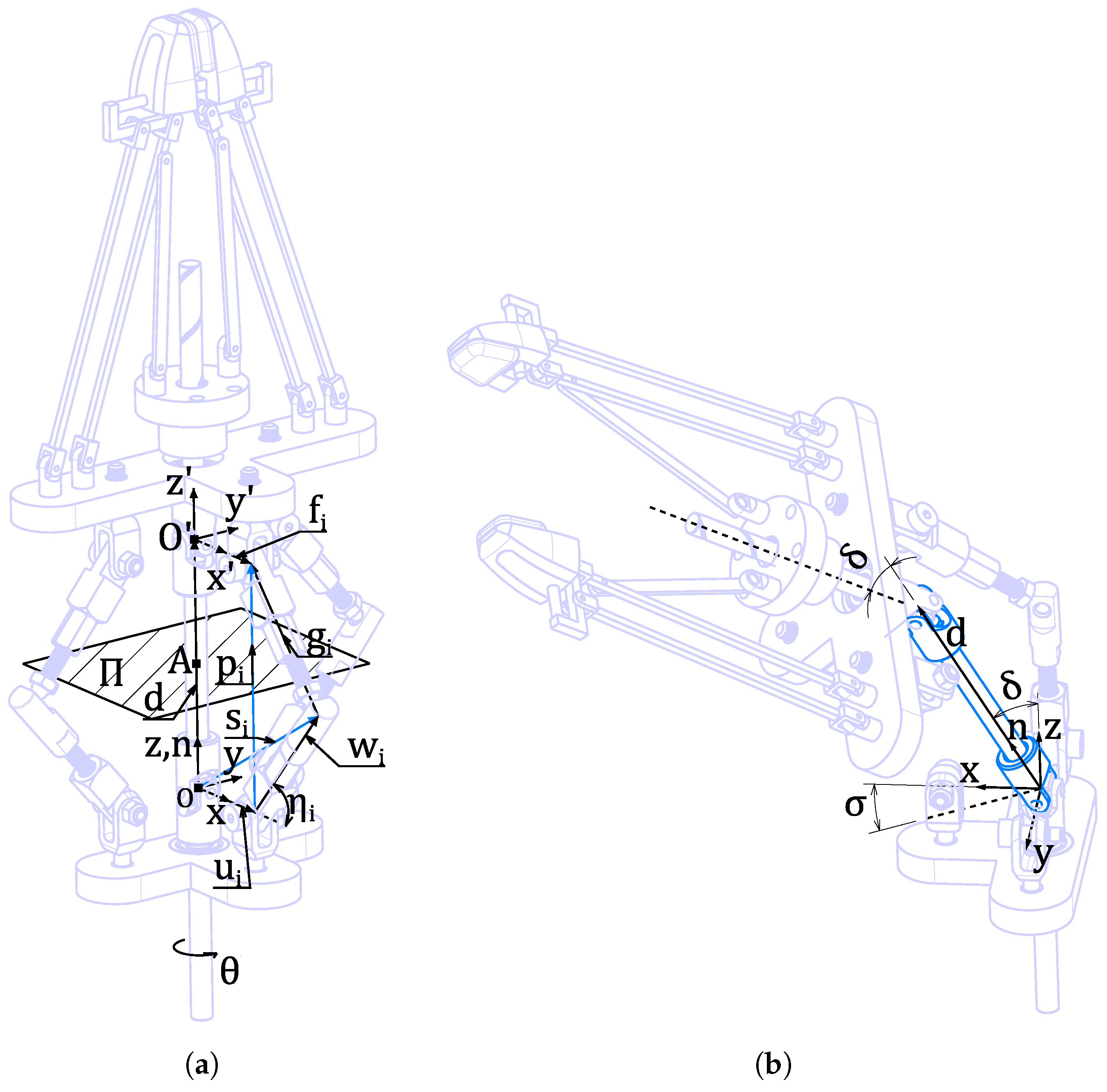
Figure 3.
Mechanical architecture of the gripper.
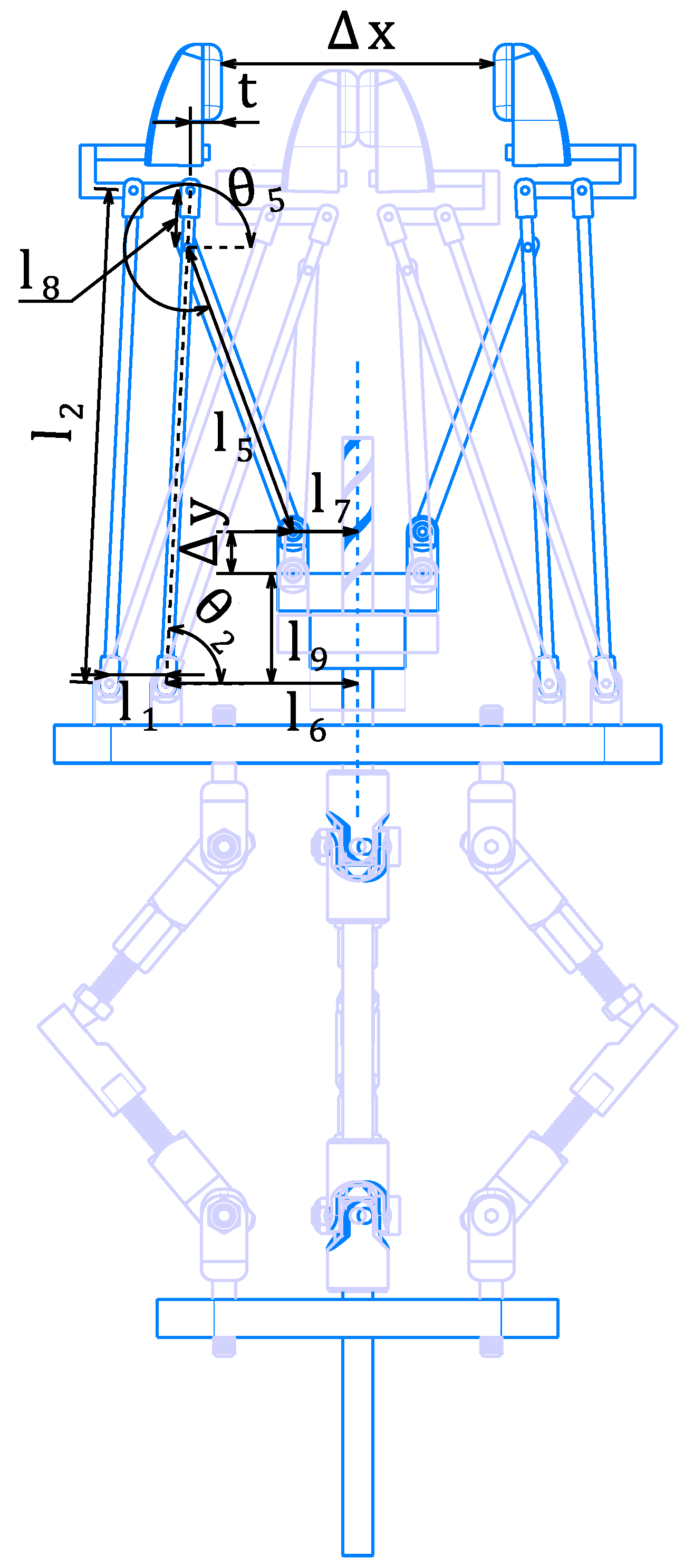
Figure 4.
The rotational workspace of the middle UU leg for , , and mm.
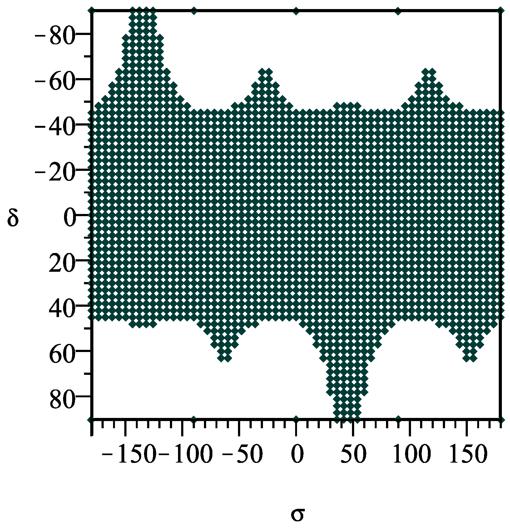
Figure 5.
The value of versus actuator angles and for , , and mm, The colour alters based on the parameter’s value.
Figure 5.
The value of versus actuator angles and for , , and mm, The colour alters based on the parameter’s value.
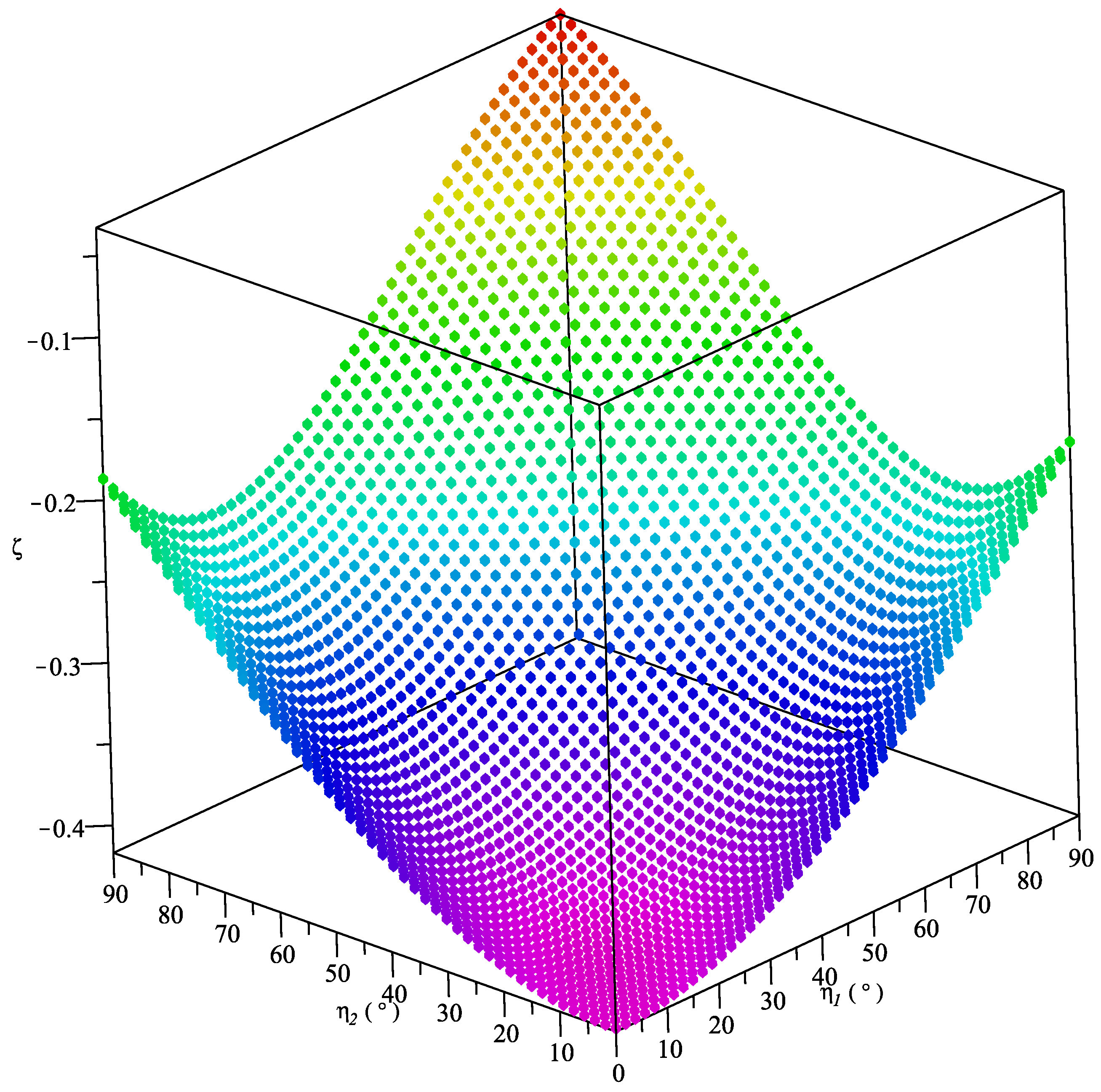
Figure 6.
Visualisation of and for the chosen coefficients , , and mm, highlighting the effect of , The colour alters based on the parameter’s value.
Figure 6.
Visualisation of and for the chosen coefficients , , and mm, highlighting the effect of , The colour alters based on the parameter’s value.
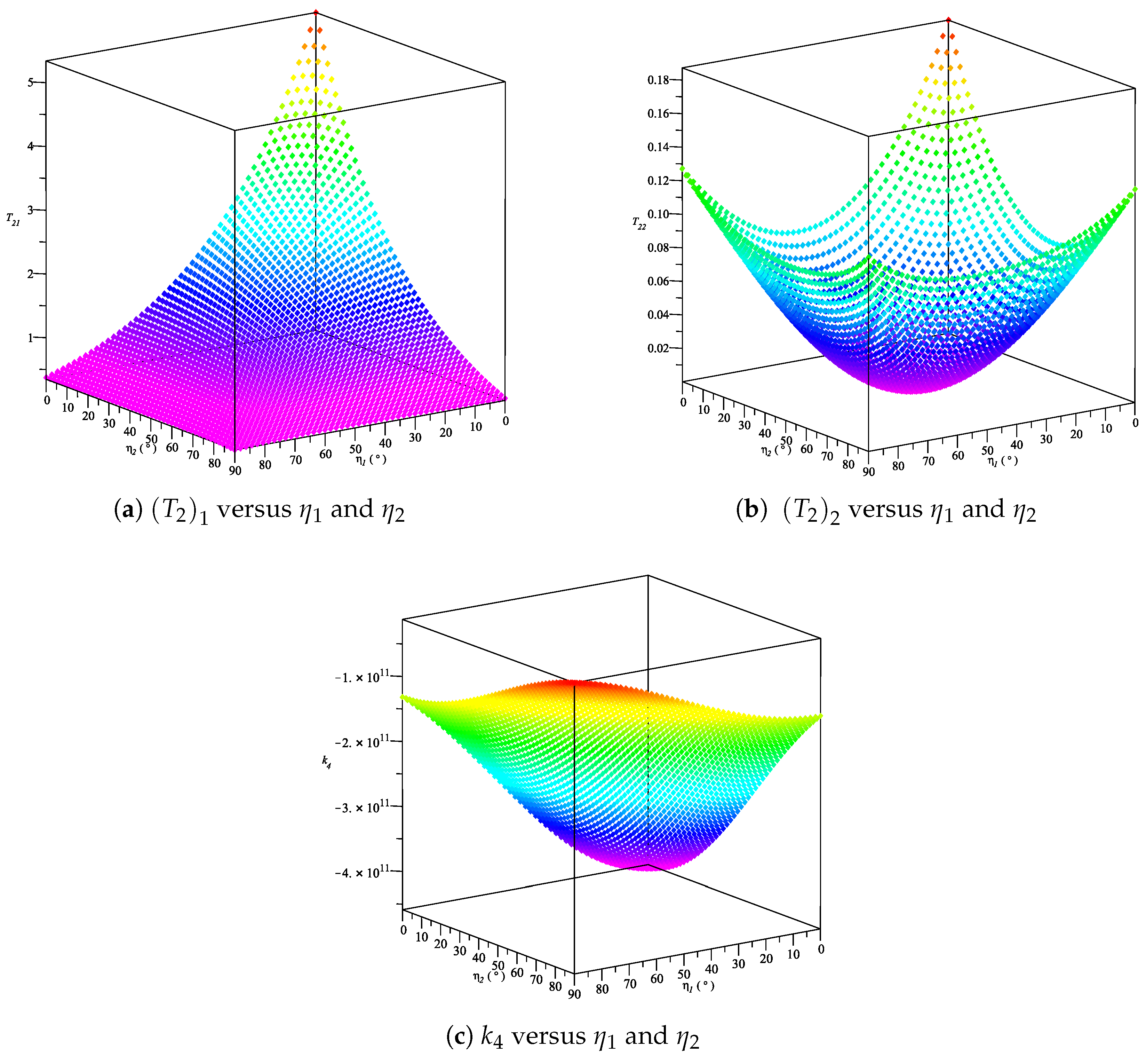
Figure 7.
(a) First actuated joint angle and (b) second actuated joint angle using inverse kinematic analytical model (circles) and results obtained from MSC Adams (solid line).
Figure 7.
(a) First actuated joint angle and (b) second actuated joint angle using inverse kinematic analytical model (circles) and results obtained from MSC Adams (solid line).

Figure 8.
The (a) tilt angle , and (b) azimuth angle , using forward kinematic analytical model (circles) and results obtained from MSC Adams (solid line).
Figure 8.
The (a) tilt angle , and (b) azimuth angle , using forward kinematic analytical model (circles) and results obtained from MSC Adams (solid line).
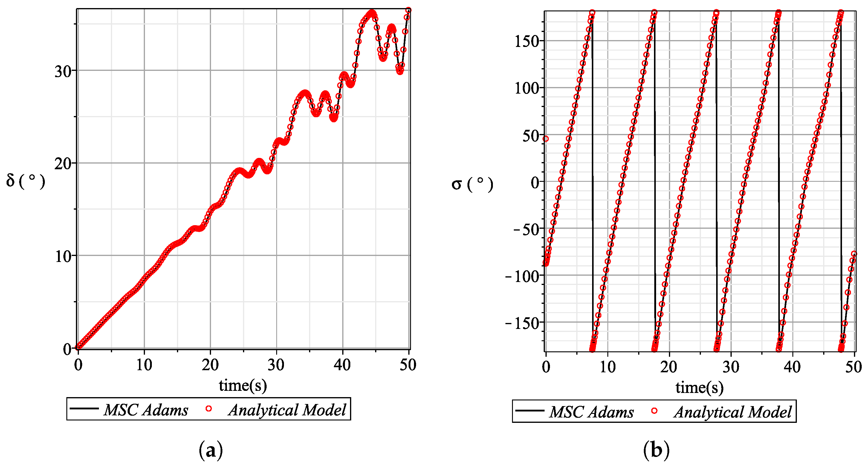
Figure 9.
(a) Proposed architecture in the study in [32] (——). (b) Proposed architecture of the current wrist-gripper assembly (——).
Figure 9.
(a) Proposed architecture in the study in [32] (——). (b) Proposed architecture of the current wrist-gripper assembly (——).

Table 1.
State-of-the-art wrist (wrist-gripper assembly) specifications.
| Reference | DOFs | Range of Motion | Parallel Gripper |
|---|---|---|---|
| Sone et al. [35] | 2 | Tilt = 90, Azimuth = | |
| Ogata et al. [36] | 2 | Pitch = , Yaw = | |
| Ueda et al. [8] | 2 | Pitch = , Yaw = | |
| Cammarata [10] | 2 | Tilt = 90, Azimuth = | |
| Ghaedrahmati and Gosselin [32] | 2 | Tilt = 90, Azimuth = | |
| OMNI Wrist III [19] | 2 | Tilt = 90, Azimuth = | |
| Kim et al. [37] | 3 | Tilt = 90, Azimuth = , Pitch = | |
| Takeda et al. [38] | 3 | Tilt = , Azimuth = , Roll = −40–0 | |
| Bazman et al. [39] | 4 | Pitch = , Yaw = , Roll = |
Disclaimer/Publisher’s Note: The statements, opinions and data contained in all publications are solely those of the individual author(s) and contributor(s) and not of MDPI and/or the editor(s). MDPI and/or the editor(s) disclaim responsibility for any injury to people or property resulting from any ideas, methods, instructions or products referred to in the content. |
© 2023 by the authors. Licensee MDPI, Basel, Switzerland. This article is an open access article distributed under the terms and conditions of the Creative Commons Attribution (CC BY) license (https://creativecommons.org/licenses/by/4.0/).
Share and Cite
MDPI and ACS Style
Ghaedrahmati, R.; Gosselin, C. Kinematic Analysis of a New 3-DOF Parallel Wrist-Gripper Assembly with a Large Singularity-Free Workspace. Actuators 2023, 12, 421. https://doi.org/10.3390/act12110421
AMA Style
Ghaedrahmati R, Gosselin C. Kinematic Analysis of a New 3-DOF Parallel Wrist-Gripper Assembly with a Large Singularity-Free Workspace. Actuators. 2023; 12(11):421. https://doi.org/10.3390/act12110421
Chicago/Turabian StyleGhaedrahmati, Ramin, and Clément Gosselin. 2023. "Kinematic Analysis of a New 3-DOF Parallel Wrist-Gripper Assembly with a Large Singularity-Free Workspace" Actuators 12, no. 11: 421. https://doi.org/10.3390/act12110421
Note that from the first issue of 2016, this journal uses article numbers instead of page numbers. See further details here.