
Evaluation Method of Soil Surface Roughness after Ditching Operation Based on Wavelet Transform


1
College of Engineering, Anhui Agricultural University, Hefei 230036, China
2
Anhui Province Engineering Laboratory of Intelligent Agricultural Machinery and Equipment, Hefei 230036, China
*
Author to whom correspondence should be addressed.
Actuators 2022, 11(3), 87; https://doi.org/10.3390/act11030087
Submission received: 12 January 2022
/
Revised: 5 March 2022
/
Accepted: 8 March 2022
/
Published: 12 March 2022
(This article belongs to the Special Issue Recent Advances and Challenges in Agricultural Robotics, Unmanned Agricultural Machinery and Autonomous Farming Technologies)
Abstract
:Soil surface roughness (SSR) is an important parameter affecting surface hydrology, erosion, gas exchange and other processes. The surface roughness of the farmland environment is directly related to the tillage process. In order to accurately characterize the random roughness (RR) parameters of the surface after ditching, a three-dimensional (3D) digital model of the surface was obtained by laser scanning under the conditions of an indoor ditching test, and the influence of oriented roughness components formed by removing ridge characteristics on the RR of the surface was analyzed by introducing the wavelet processing method. For this reason, four groups of ditching depths and two types of surface conditions (whether the surface was agglomerated or not) were designed in this paper. By comparing the root mean squared height (RMSH) and correlation length (CL) data calculated before and after wavelet processing under each group of tests, it was concluded that the RMSH values of the four groups before and after wavelet processing all change more than 200%, the change amplitude reached 271.02% under the treatment of 12 cm ditching depth, meanwhile, the average CL value of five cross-sections under each group of ditching depths decreased by 1.43–2.28 times, which proves that the oriented roughness component formed by furrows and ridges has a significant influence on the calculation of RR. By further analyzing the roughness value differences of clods and pits in different directions and local areas before and after wavelet transform, it was shown that the wavelet transform can effectively remove the surface anisotropy characteristics formed in the tillage direction and provide a uniform treatment method for the evaluation of surface RR at different ditching depths.
1. Introduction
Soil surface roughness (SSR), defined as the spatial variation of soil surface height, is one of the important soil surface characteristics affecting surface hydrology, erosion, gas exchange and other processes [1,2]. It is also an important parameter that affects the stable walking of small agricultural robots in the field [3,4]. Changes of SSR in farmland are mainly controlled by natural factors such as agricultural tillage and field management activities, wind, rain, and gravity, as well as the physical and chemical properties of soil itself [5]. Human agricultural activities can dramatically change surface roughness in a short time, while natural factors change SSR more slowly [6]. In order to quantitatively describe SSR changes, most previous studies were mainly represented by root mean squared height (RMSH), correlation length (CL) and autocorrelation function (ACF) of soil surface. Given the values of the above three parameters, the height changes of soil surface can be determined.
The roughness characteristics of farmland soil surface are mainly manifested in three scales of small, medium, and large [7]: (1) random roughness (RR) of surface height variation caused by random spatial arrangement of individual clods; (2) oriented roughness of surface height changes due to rows or furrows generated by agricultural machinery operation; and (3) terrain roughness, which is the result of height variations on topographic scales. RR, which can truly reflect the quality of surface tillage (size of surface clods or aggregates, geometric dimensions of surface bulges or pits), is a key factor affecting seedling emergence and growth uniformity.
The current research on SSR mainly focuses on two aspects: measurement methods and evaluation methods, among them, measurement methods can be divided into two categories: contact and non-contact. The pin meter method [8] and the chain method [9] are the main contact measuring methods, they are simple and feasible in field measurement, but there are problems such as limited measuring range, labor-intensiveness and destruction of surface structure. The non-contact measuring methods do not touch the soil during the measuring process and can accurately measure the soil surface elevation information. The measuring process is usually carried out utilizing laser scanner [10,11], camera [12,13], sound wave sensor [14], infrared [15], etc. Laser scanning equipment based on the principle of laser ranging can be classified as single-point laser [16], line laser [17] and 3D laser [18]. While the measurement area and measurement efficiency of the three are successively improved, the equipment cost also increases successively. Photogrammetric methods have also been widely used in the 3D reconstruction of farmland surfaces, but photogrammetric methods are very demanding to illumination conditions and are rarely used in field ditch environments [19]. Compared with laser and camera technology, acoustic wave measurement and infrared measurement technology do not have advantages in measurement efficiency and accuracy, so they are less applied [20]. In recent years, unmanned aerial vehicle (UAV) technology has also been applied in SSR measurement. Compared with ground measurement technology, UAV has higher efficiency and larger measuring area, but also higher cost [21,22].
With the rapid development of sensor technology, the commonly used non-contact measurement methods can meet the measurement requirements of farmland SSR in terms of measurement accuracy. However, since the soil surface after agricultural operations usually produces ridge structures and small ditches along the farming direction, the existence of this oriented roughness will lead to the anisotropy and multi-scale of SSR [11], so there are still many problems in the quantitative method and evaluation basis of roughness parameters [19]. Although many parameters and indexes can be used to quantify surface roughness, none of them are universally applicable [23], especially in the presence of oriented roughness components formed by ridges and furrows, the calculation results of quantitative parameters such as RMSH and CL are quite different from the surface evaluation parameters of the non-oriented roughness under the same tillage intensity [24]. Therefore, quantitative parameters such as RMSH and CL cannot be directly correlated with farming intensity. In order to solve the above problems and make the oriented roughness parameters not affect the evaluation results of RR, we introduce a wavelet-based method to remove the oriented roughness information introduced by the undulation of ridges and furrows, thus accurately describing the RR information contributed by bulges or pits formed by local surface undulations or clods. Furthermore, this method can accurately quantify the RR of cultivated surface without the influence of oriented roughness component.
The purpose of this study is to quantify the impact of different ditching depths and surface agglomeration (formed by simulated rainfall) on the RR of the surface based on the above method. In order to accurately obtain the influence relationship, seedbeds with ditching depths of 5 cm and 8 cm under original surface environment and 10 cm and 12 cm under surface agglomeration were created in an indoor soil bin environment, four groups of tests in total. The laser radar is used to collect the 3D elevation data of the soil surface after the ditching operation, and the data is processed by MATLAB to extract the wavelet datum reflecting the change of the ridges and furrows, so as to calculate the random surface roughness after removing the oriented roughness. Through the analysis and comparison of the obtained data, the influence relationship of the soil under different ditching depths and whether the surface is agglomerated on the random surface roughness is obtained, and an SSR evaluation method that eliminates the influence of oriented roughness is proposed.
2. Materials and Methods
2.1. Design of Ditching Test and Measurement of Surface Roughness
2.1.1. Indoor Soil Bin Test Design
A 4-m-long and 0.8-m-wide soil bin was designed in the Midwest Comprehensive Building of Anhui Agricultural University. The ditching shovel (Figure 1) was installed on a horizontally moving support driven by a motor. The soil in the soil bin was filled up and four sets of experiments were set up. The ditching depths were 5 cm, 8 cm, 10 cm and 12 cm respectively. The ditching depths of 10 cm and 12 cm were treated with the same amount of artificial precipitation. The Initial landform is shown in Figure 2. We could adjust the ditching depth of the ditching shovel through the installation hole position. After starting the test equipment, the motor drove the ditching shovel to create a furrow on the ground, as shown in Figure 3.
2.1.2. Preparation and Measurement of SSR Measuring Device
The roughness measuring device was installed on the surface after tillage to measure SSR. The non-contact surface roughness measurement device includes laser radar (LMS511–10100 PRO), bracket, stepper motor, motor driver and portable computer. The device is shown in Figure 4. Among this, a linear guide rail was installed on the bracket, and the laser radar was fixedly connected to the guide rail, which could move linearly under the drive of a stepper motor. The stepper motor is controlled by interactive software in the portable computer, which can realize precise rotation. After finishing the laser radar sampling parameters setting and stepper motor moving speed setting, the equipment could start to work. During the LiDAR moving with the slider, the collected soil surface elevation data was transmitted to the portable computer via Ethernet communication. The test process and data collection process is shown in Figure 5.
2.2. Evaluation of SSR
2.2.1. Data Preprocessing
The data collected by LiDAR is recorded in polar coordinates, so it needs to be converted into rectangular coordinates. To this end, a Python program was developed to achieve rapid conversion and generate the required 3D coordinate data. In order to avoid the boundary effect caused by the boundary of soil bin, 3D point cloud data were imported into MATLAB and cut to a distance of 5 cm from the edge of soil bin. The interpolation processing was carried out on the LiDAR data generated from each set of tests, and the regular elevation data with 5 mm interval in the X and Y directions were obtained for subsequent calculation and processing.
2.2.2. Extraction of Random Surface Roughness Features Based on Wavelet Transform
In order to eliminate the influence of oriented roughness such as ridges and furrows on the RRS evaluation, this study draws on the experience of detecting clods based on the wavelet method introduced by Vannier et al. [25], combines the application of wavelet transform analysis in evaluating 3D surface morphology of parts and automatic monitoring [26,27,28] and applies wavelet transform to the analysis of soil roughness.
(1) Mathematical Model and Principle
Decompose the surface elevation into an approximate value and the sum of N details , where N represents the number of wavelet decomposition, under different decomposition times N:
The approximations and details of the surface are computed by recurrence:
where denotes the summation of the horizontal, vertical and diagonal detail surfaces:
At each intermediate level are calculated using decimated and undecimated algorithms to generate sub-images with the same size as the original image. In fact, the frequency plan is subdivided into two parts, low frequency and high frequency, along each dimension x and y. The approximation is the low-low frequency part, the horizontal detail the high-low frequency part, the vertical detail is the low-high frequency part, and the diagonal detail is the high-high frequency part [29].
(2) Optimal Wavelet Selection and Number of Wavelet Decomposition
Wavelet transform contains many wavelets basis functions, and the results of wavelet datum extraction using different wavelet functions are quite different [30]. Therefore, the selection of appropriate wavelet functions becomes a key point. As far as the current selection criteria are concerned, there is no uniform standard, and the selection is generally based on experience or experiment. In this paper, the appropriate wavelet function is selected by comparing the reconstruction error of common wavelet functions to data.
The extraction accuracy of wavelet datum is also related to the decomposition times of wavelet [30]. In this study, according to the energy conservation principle of wavelet decomposition and the characteristics of exponential change [31], the high-frequency energy under decomposition coefficients of each layer is fitted exponentially in order. When the energy percentage of a layer deviates from the curve, the number of previous decomposition layers is the optimum number of wavelet decompositions. One of the 3D elevation surface data measured in this experiment is decomposed nine times, and the high-frequency energy percentage under the decomposition coefficient of each layer after wavelet decomposition is calculated by programming. The exponential function is used for fitting, as shown in Figure 6. The fitting curve clearly shows that the optimal wavelet decomposition number is five times.
2.2.3. Evaluation Parameters of 3D Morphology
In the evaluation study of surface roughness, predecessors have listed a variety of evaluation parameters [32,33]. RMSH and CL are commonly used parameters to characterize the random surface roughness.
RMSH reflects the degree of deviation of the surface micro-topography from the average height and plays an important role in evaluating the soil quality after farming with agricultural machinery. Since this study is based on discrete point data obtained by LiDAR scanning, RMSH can be expressed as:
where M is the number of columns in the sampling area, N is the number of rows in the sampling area, is the number of columns, is the number of rows, is the height of sampling points corresponding to row and , and is the average height of all sampling points.
Different from RMSH, CL reflects the change of soil surface height in the horizontal direction and reflects the correlation between sampling points. CL is determined by the normalized ACF. For discrete data, the ACF is defined as:
where is the distance between two sampling points, let be the distance between two adjacent coordinates in the coordinate direction, then . n is the number of sampling points and is an integer greater than or equal to 1. When the correlation function , the interval is called CL.
2.3. Data Analysis
Each group of test data after data preprocessing in Section 2.2.1 is processed by wavelet transform to obtain two types of digital elevation models (DEM) before and after wavelet processing. To analyze the influence of sampling window size on SSR calculation results, RMSH values (window width is the total width of DEM) of window data corresponding to three lengths (200 mm, 400 mm and 600 mm) along the tillage direction were counted. Means and standard deviations of RMSH were calculated in ten areas randomly selected under each window length. The CL results were calculated by intercepting five cross-section data at equal distances perpendicular to the farming direction. In addition, in order to study the anisotropic characteristics of SSR, three sections perpendicular to tillage direction (0°, 45° and 90°) were selected for RMSH and CL calculation in four test treatments to compare SSR data differences in different directions.
3. Results and Discussion
3.1. Digital Model of Soil Surface under Different Ditching Depths
According to the data preprocessing in Section 2.2.1, the 3D digitized models of soil surface at four different depths of ditching were established by MATLAB, as shown in Figure 7.
It can be seen from Figure 7 that due to the action of the ditching shovel, furrows of different depths are formed on the ground along the cultivation direction. In the test with ditching depths of 10 cm and 12 cm, due to the agglomeration of the surface, it can be clearly seen that there are clods or large aggregates on the surface. At the same time, from the pictures of the above four ditching depths, there is obvious anisotropy in the roughness of cross-sections in different directions of the surface due to the existence of furrows and ridges, which poses a challenge to the accurate evaluation of surface roughness.
3.2. Digital Model of Soil Surface after Wavelet Transform
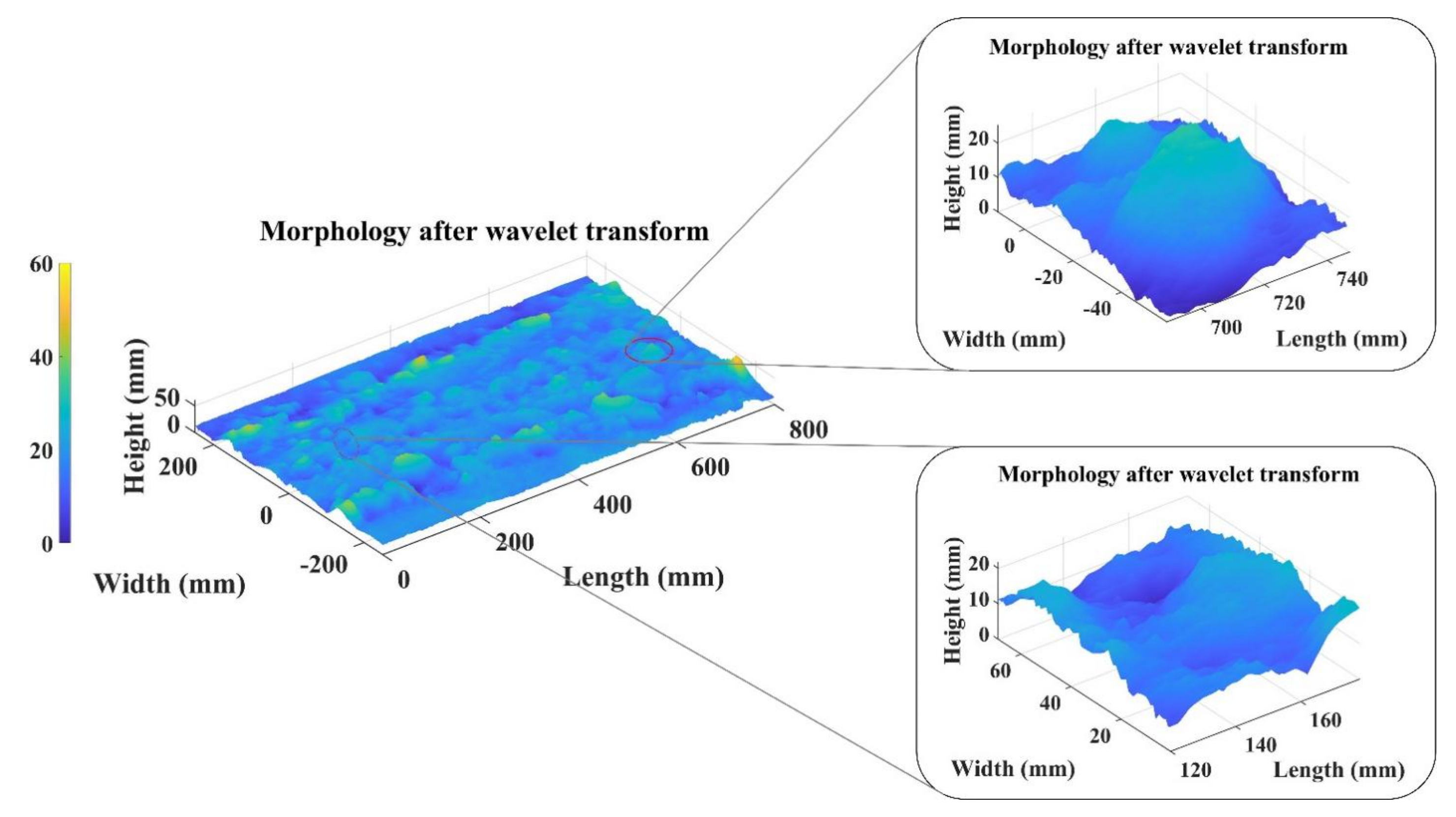
Based on the four digital models of the soil surface with different ditching depths obtained in Section 3.1, the corresponding wavelet datum plane is extracted according to the above wavelet transform principle. By subtracting the height data of corresponding points on the wavelet datum from the elevation data of the original ground surface, we can obtain the surface elevation data without the orientation trend of ridges and furrows. As shown in Figure 8, the 3D digitized model pictures under different ditching depths are shown, in which the left picture under each depth is the extracted wavelet datum surface and the right picture is the DEM of soil surface after wavelet transform.
It can be seen from Figure 8 that the soil surface after wavelet processing no longer shows the phenomenon of ridges and furrows caused by the cultivation direction, and the anisotropy of the roughness parameters in different cross-sections of the soil surface is significantly weakened. At the same time, compared with Figure 7 and Figure 8, it can be seen that the surface micro-undulations formed by clods or soil aggregates on the soil surface are well restored after wavelet transform, and the RR characteristics of the soil surface are not deformed due to wavelet transform.
Figure 9 shows one digital model cross-section of the soil surface under different ditching depths and the corresponding cross-section of the wavelet datum. It can be seen from the curve in the figure that the extraction of the wavelet datum plane is very accurate, which can reflect the fluctuation trend of the soil surface accurately. Especially for the two treatments with a ditching depth of 5 cm and 8 cm, due to the small soil particle size in the soil bin, the cross-section of the wavelet datum is almost coincident with the corresponding cross-section of the soil surface after ditching.
3.3. Analysis of Surface Roughness Calculation Results
3.3.1. Analysis of RMSH Calculation Results
According to the data processing method described in Section 2.3, the surface roughness parameters under four ditching depths were statistically analyzed, and the RMSH results before and after soil surface wavelet transform under different ditching depths and different sampling window sizes were obtained, as shown in Figure 10. Among these, Figure 10a shows two operation depths without simulated rainfall treatment, and Figure 10b shows two operation depths with agglomeration on the surface after simulated rainfall treatment.
It can be seen that with the increase of ditching depth, the value of RMSH is positively correlated. The two depths of 5 cm and 8 cm have smaller soil disturbance areas, so there is no significant increase in the number of RMSH. From the tests of two groups of surface after simulated rainfall treatment (10 cm and 12 cm), it can be seen that in addition to the impact of the increase of ditching depth on RMSH, the size of soil disturbance area, clods or soil aggregate changes greatly compared with the untreated surface, so the RMSH values also show great differences. As the sampling window increases in the farming direction, although the mean value of RMSH does not show a great difference in value, the standard deviation of the results of 10 samplings gradually decreases, which shows that a larger sampling window can make the calculation results more stable. Many studies have thoroughly discussed the impact of the size of sampling window on the roughness evaluation results, and this study will not be carried out again [34].
Table 1 shows the comparison of RMSH values of different ditching depths before and after wavelet transform. It can be seen from the most concerned issues in this study that the RMSH values have changed greatly before and after wavelet processing. The changing amplitude of the RMSH values of the four groups of processing before and after wavelet processing exceeded 200%, and the change amplitude of the largest group of data reached 271.02%. Significantly, the RMSH values after wavelet processing were relatively close, in which the RMSH values after wavelet transform in 5 cm and 8 cm groups were almost equal, and the RMSH values after wavelet transform in 10 cm and 12 cm groups were only 0.54 mm. It can be considered that the RMSH values after wavelet processing are not significantly different when the difference in ditching depths is small (the difference is 2 cm).
3.3.2. Analysis of CL Calculation Results
In the four experimental treatments, five soil cross-sections before and after wavelet transform are selected equidistantly perpendicular to the farming direction, and the CL of each cross-section data is calculated according to Equation (6). The results are shown in Table 2.
Combining the ACF of one group of data (Figure 11), it can be seen that the cross-sectional CL after wavelet processing was reduced, the average CL value of five cross-sections under each group of ditching depths decreased by 1.43–2.28 times, and the five groups of cross-sectional CL data processed by each experiment maintain a good consistency. As the ditching depth increased, the value of CL also shows an increasing trend, especially after the surface agglomerates, CL increased significantly, from 23.42 mm at a depth of 8 cm to 41.89 mm at a depth of 10 cm. By comparing the CL after wavelet processing, it can be found that the difference of CL under different ditching depths is not obvious, which shows that the wavelet processing has removed the influence of the oriented roughness produced by ridges and furrows on the CL.
Figure 11 also clearly shows the changing trend of the ACF curve before and after wavelet processing. In the original soil surface, the number of peak and valley values of surface ACF is small, which mainly reflects the distribution of furrows and ridges. After wavelet transform, there are multiple extreme points of surface ACF, which is mainly the result of the distribution of clods or aggregates on the surface.
3.3.3. Comparative Analysis of Roughness Parameters in Different Directions
In the previous analysis, it was mentioned that the direction of the ditching operation produced anisotropic characteristics of the surface roughness. Previous studies in this area only focused on the comparison of roughness values in different directions [35]. In order to further explore the impact of different directions on surface roughness parameters before and after wavelet processing, three cross-sections perpendicular to tillage direction 0°, 45° and 90° were selected for RMSH and CL calculation in four test treatments. The results are shown in Table 3.
It can be seen that among the four groups of data before wavelet transform, the RMSH in the 90° direction is the smallest, because the cross-section in this direction is parallel to the direction of the ditching, and the structure of the furrows and ridges has little impact on the calculation of RMSH, while the cross-sections in the 0° and 45° directions span the furrows and ridges, so the corresponding RMSH values are both large, this is consistent with the previous research conclusion [24,35]. Comparing the results after wavelet processing, it can be seen that the RMSH values of the cross-sections at 0° and 45° are significantly different before and after the wavelet processing, and the value of CL also has the same trend, which is consistent with the results in Section 3.3.1 and Section 3.3.2. In comparison, the RMSH value after wavelet processing in the 90° direction cross-section has a smaller change than before. From the results of wavelet processing, it can also be seen that the RMSH values under each experimental treatment have relatively small differences in the three cross-sectional directions, which also verifies that wavelet processing is very effective in removing the oriented roughness formed by ridges and furrows.
3.4. Impact of Ridges and Furrows on Evaluation of Surface Roughness in Local Area
The oriented roughness caused by the undulation of ridges and furrows formed by tillage will significantly affect the calculated value of RR, and with the increase of tillage depth, the surface elevation data generated by the ridge and furrow effect will weaken the contribution of RR generated by the random distribution of clods to the calculated value of roughness, while the effect of ridge and furrow effect can be effectively eliminated by wavelet processing. In order to further verify the above discussion, 3D elevation data of soil surface in Test 3 were selected as the research object, and two areas on the slope of the ditch were intercepted, one area with clods on the slope and the other area with pits on the slope, as shown in Figure 12. According to Equation (5), the initial RMSH of the two areas were calculated respectively, and then, the soil surface of Test 3 was processed with wavelet transform and the same location above was intercepted (Figure 13), and finally, RMSH was calculated respectively. The RR changes of selected areas before and after wavelet transform were analyzed and the results are shown in Table 4.
From the statistical data analysis in Table 4, it can be seen that after the wavelet transform, the roughness of the two selected areas change by 47.78% and 46.41% respectively, with obvious differences in value before and after transformation. Based on the above two situations, the influence of ridges and furrows undulations on the calculation of soil roughness is verified, and this effect can be effectively removed by using wavelet transform. Compared with the scheme of removing the tilt trend [32], this method does not need to remove the trend separately for each small area to be calculated, and has higher processing efficiency. This study provides a unified calculation standard for random surface roughness evaluation under different tillage intensities.
4. Conclusions
In this study, we proposed a method based on wavelet processing to remove the oriented roughness formed by rows in indoor soil bin test and provide a unified evaluation method for the RR formed by clods distribution under different ditching depths. Based on this method, we have studied the influence of different ditching depths and whether the surface is agglomerated on the RR of the soil surface, and obtained the following conclusions:
(1) By comparing the RMSH and CL data calculated before and after the wavelet processing in each group of experiments, it can be seen that the SSR results before and after the wavelet processing have changed significantly. The RMSH values of the four groups before and after the wavelet processing all change more than 200%, and the change amplitude reached 271.02% under 12 cm ditching depth treatment—this result indicates that if the oriented roughness component formed by the furrow and ridge features is not removed, the contribution of clods or local pits to the RR will be severely weakened.
(2) From the SSR data results of four groups of tests, it can be seen that with the increase of ditching depths, the results of RMSH are positively correlated regardless of whether the DEM of each group of tests is processed by wavelet or not, and the value of CL maintains an increasing trend basically, in particular, after the surface agglomeration is processed, the results of RMSH show a significant upward trend. In contrast, the results of CL values at different depths after wavelet processing are relatively close. We also studied the changes of the roughness data of cross-sections in different directions before and after wavelet processing, and further verified that wavelet processing can remove the influence of oriented roughness component on roughness result evaluation.
(3) By extracting the clods and pits at the same position on the DEM before and after wavelet processing, the changes in the results of RMSH are counted. It can be seen that after the wavelet transform, the roughness of the two selected areas change by 47.78% and 46.41% respectively, which proves that the wavelet processing can also remove the slope trend on a small scale, and the statistical results after wavelet transform can better represent the influence of clods or pits on RR.
Author Contributions
Conceptualization, L.C.; methodology, L.L.; software, Q.B.; validation, Q.Z.; data analysis, Q.B.; investigation, D.B.; resources, L.C.; data curation, L.L.; writing—original draft preparation, L.L.; writing—review and editing, L.C.; supervision, J.T.; project administration, L.L.; funding acquisition, L.C. All authors have read and agreed to the published version of the manuscript.
Funding
This study was funded by Universities Natural Science Research Project of Anhui Province (Grant No. KJ2020A0105) and Collaborative Innovation Project of Colleges and Universities of Anhui Province (Grant No. GXXT-2020-011).
Institutional Review Board Statement
Not applicable.
Informed Consent Statement
Not applicable.
Data Availability Statement
The data presented in this study are available on request from the corresponding author.
Conflicts of Interest
The authors declare no conflict of interest.
References
- Darboux, F.; Davy, P.; Gascuel-Odoux, C.; Huang, C. Evolution of soil surface roughness and flowpath connectivity in overland flow experiments. Catena 2002, 46, 125–139. [Google Scholar] [CrossRef]
- Peñuela, A.; Javaux, M.; Bielders, C.L. How do slope and surface roughness affect plot-scale overland flow connectivity? J. Hydrol. 2015, 528, 192–205. [Google Scholar] [CrossRef]
- Zhiqang, L.; Liqing, C.; Quan, Z.; Xianyao, D.; Lu, Y. Control of a path following caterpillar robot based on a sliding mode variable structure algorithm. Biosyst. Eng. 2019, 186, 293–306. [Google Scholar]
- Liqing, C.; Pinpin, W.; Peng, Z.; Quan, Z.; Jin, H.; Qingjie, W. Performance analysis and test of a maize inter-row self-propelled thermal fogger chassis. Int. J. Agric. Biol. Eng. 2018, 11, 100–107. [Google Scholar]
- Xingming, Z.; Tao, J.; Xiaofeng, L.; Yanling, D.; Kai, Z. The temporal variation of farmland soil surface roughness with various initial surface states under natural rainfall conditions. Soil Tillage Res. 2017, 170, 147–156. [Google Scholar] [CrossRef]
- Gessesse, G.D.; Fuchs, H.; Mansberger, R.; Klik, A.; Rieke-Zapp, D.H. Assessment of erosion, deposition and rill development on irregular soil surfaces using close range digital photogrammetry. Photogramm. Rec. 2010, 25, 299–318. [Google Scholar] [CrossRef]
- Beaudoin, A.; Le Toan, T.; Gwyn, Q. SAR observations and modeling of the C-band backscatter variability due to multiscale geometry and soil moisture. IEEE Trans. Geosci. Remote Sens. 1990, 28, 886–895. [Google Scholar] [CrossRef]
- Moreno, R.G.; Alvarez, M.D.; Requejo, A.S.; Delfa, J.V.; Tarquis, A. Multiscaling analysis of soil roughness variability. Geoderma 2010, 160, 22–30. [Google Scholar] [CrossRef]
- Thomsen, L.; Baartman, J.; Barneveld, R.; Starkloff, T.; Stolte, J. Soil surface roughness: Comparing old and new measuring methods and application in a soil erosion model. Soil 2015, 1, 399–410. [Google Scholar] [CrossRef] [Green Version]
- Polyakov, V.; Nearing, M. A simple automated laser profile meter. Soil Sci. Soc. Am. J. 2019, 83, 327–331. [Google Scholar] [CrossRef] [Green Version]
- Xingming, Z.; Lei, L.; Chunmei, W.; Leran, H.; Tao, J.; Xiaojie, L.; Zhuangzhuang, F. Measuring surface roughness of agricultural soils: Measurement error evaluation and random components separation. Geoderma 2021, 404, 115393. [Google Scholar] [CrossRef]
- Xu, L.; Zheng, C.; Wang, Z.; Nyongesah, M. A digital camera as an alternative tool for estimating soil salinity and soil surface roughness. Geoderma 2019, 341, 68–75. [Google Scholar] [CrossRef]
- Grundy, L.; Ghimire, C.; Snow, V. Characterisation of soil micro-topography using a depth camera. MethodsX 2020, 7, 101144. [Google Scholar] [CrossRef] [PubMed]
- Lou, S.; He, J.; Lu, C.; Liu, P.; Li, H.; Zhang, Z. A Tillage Depth Monitoring and Control System for the Independent Adjustment of Each Subsoiling Shovel. Actuators 2021, 10, 250. [Google Scholar] [CrossRef]
- Mohammadi, F.; Maleki, M.R.; Khodaei, J. Control of variable rate system of a rotary tiller based on real-time measurement of soil surface roughness. Soil Tillage Res. 2022, 215, 105216. [Google Scholar] [CrossRef]
- Ehlert, D.; Adamek, R.; Horn, H.J. Laser rangefinder-based measuring of crop biomass under field conditions. Precis. Agric. 2009, 10, 395–408. [Google Scholar] [CrossRef]
- Jensen, T.; Karstoft, H.; Green, O.; Munkholm, J.L. Assessing the effect of the seedbed cultivator leveling tines on soil surface properties using laser range scanners. Soil Tillage Res. 2017, 167, 54–60. [Google Scholar] [CrossRef]
- Foldager, F.F.; Pedersen, J.M.; Haubro Skov, E.; Evgrafova, A.; Green, O. Lidar-based 3d scans of soil surfaces and furrows in two soil types. Sensors 2019, 19, 661. [Google Scholar] [CrossRef] [Green Version]
- Riegler, T.; Rechberger, C.; Handler, F.; Prankl, H. Image processing system for evaluation of tillage quality. Landtechnik 2014, 69, 125–131. [Google Scholar]
- Jiang, C.; Fang, H.; Wei, S. Review of Land Surface Roughness Parameterization Study. Adv. Earth Sci. 2012, 27, 292–303. [Google Scholar]
- Fanigliulo, R.; Antonucci, F.; Figorilli, S.; Pochi, D.; Pallottino, F.; Fornaciari, L.; Costa, C. Light drone-based application to assess soil tillage quality parameters. Sensors 2020, 20, 728. [Google Scholar] [CrossRef] [PubMed] [Green Version]
- Onnen, N.; Eltner, A.; Heckrath, G.; Van Oost, K. Monitoring soil surface roughness under growing winter wheat with low-altitude UAV sensing: Potential and limitations. Earth Surf. Process. Landf. 2020, 45, 3747–3759. [Google Scholar] [CrossRef]
- Martinez-Agirre, A.; Alvarez-Mozos, J.; Gimenez, R. Evaluation of surface roughness parameters in agricultural soils with different tillage conditions using a laser profile meter. Soil Tillage Res. 2016, 161, 19–30. [Google Scholar] [CrossRef] [Green Version]
- Turner, R.; Panciera, R.; Tanase, M.A.; Lowell, K.; Hacker, J.M. Estimation of soil surface roughness of agricultural soils using airborne LiDAR. Remote Sens. Environ. 2014, 140, 107–117. [Google Scholar] [CrossRef]
- Vannier, E.; Ciarletti, V.; Darboux, F. Wavelet-based detection of clods on a soil surface. Comput. Geosci. 2009, 35, 2259–2267. [Google Scholar] [CrossRef]
- Barton, D.; Federhen, J.; Fleischer, J. Retrofittable vibration-based monitoring of milling processes using wavelet packet transform. Procedia CIRP 2021, 96, 353–358. [Google Scholar] [CrossRef]
- Hou, W.; Zhang, D.; Wei, Y.; Guo, J.; Zhang, X. Review on computer aided weld defect detection from radiography images. Appl. Sci. 2020, 10, 1878. [Google Scholar] [CrossRef] [Green Version]
- Wang, H.; Chi, G.; Jia, Y.; Ge, C.; Yu, F.; Wang, Z.; Wang, Y. Surface roughness evaluation and morphology reconstruction of electrical discharge machining by frequency spectral analysis. Measurement 2021, 172, 108879. [Google Scholar] [CrossRef]
- Vannier, E.; Dusséaux, R.; Taconet, O.; Darboux, F. Wavelet-based clod segmentation on digital elevation models of a soil surface with or without furrows. Geoderma 2019, 356, 113933. [Google Scholar] [CrossRef]
- Liu, Y.; Zheng, Y.; Li, J.; Jing, D.; Gu, Y. Study on Surface Morphology of Vibration Assisted Cutting. Procedia CIRP 2018, 71, 65–70. [Google Scholar] [CrossRef]
- Youming, Z. Wavelet Packet Time-Frequency Analysis and Its Property. J. Vib. Meas. Diagn. 2009, 29, 170. [Google Scholar]
- Xingming, Z.; Kai, Z.; Xiaojie, L.; Yangyang, L.; Jianhua, R. Improvements in farmland surface roughness measurement by employing a new laser scanner. Soil Tillage Res. 2014, 143, 137–144. [Google Scholar] [CrossRef]
- Yang, P.; Jiang, S. The study on the 3D assessment of surface roughness. Mach. Des. Res. 2002, 18, 64–67. [Google Scholar]
- Sanner, A.; Nöhring, W.G.; Thimons, L.A.; Jacobs, T.D.B.; Pastewka, L. Scale-dependent roughness parameters for topography analysis. Appl. Surf. Sci. Adv. 2022, 7, 100190. [Google Scholar] [CrossRef]
- Zhixiong, L.; Nan, C.; Perdok, U.; Hoogmoed, W. Characterisation of Soil Profile Roughness. Biosyst. Eng. 2005, 91, 369–377. [Google Scholar] [CrossRef]
Figure 1.
Ditching shovel.
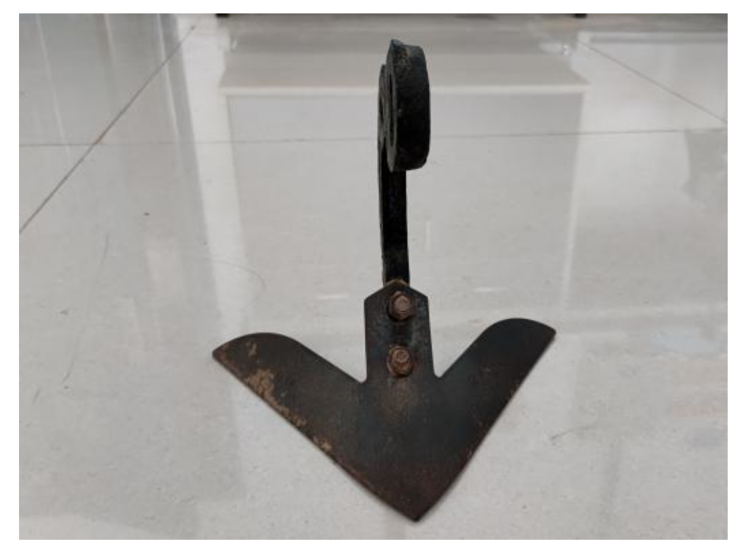
Figure 2.
Initial landform.
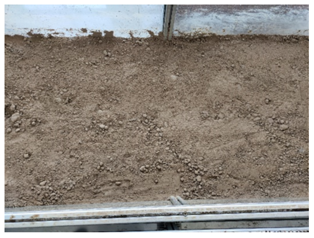
Figure 3.
Landform after ditching.
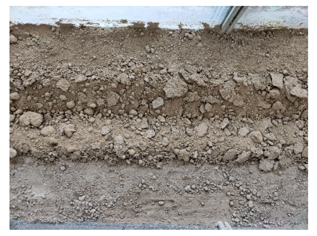
Figure 4.
Measuring device.
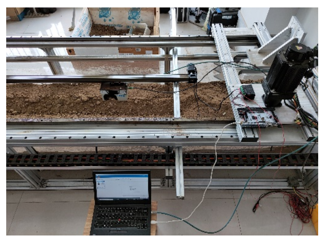
Figure 5.
The test process and data collection process.
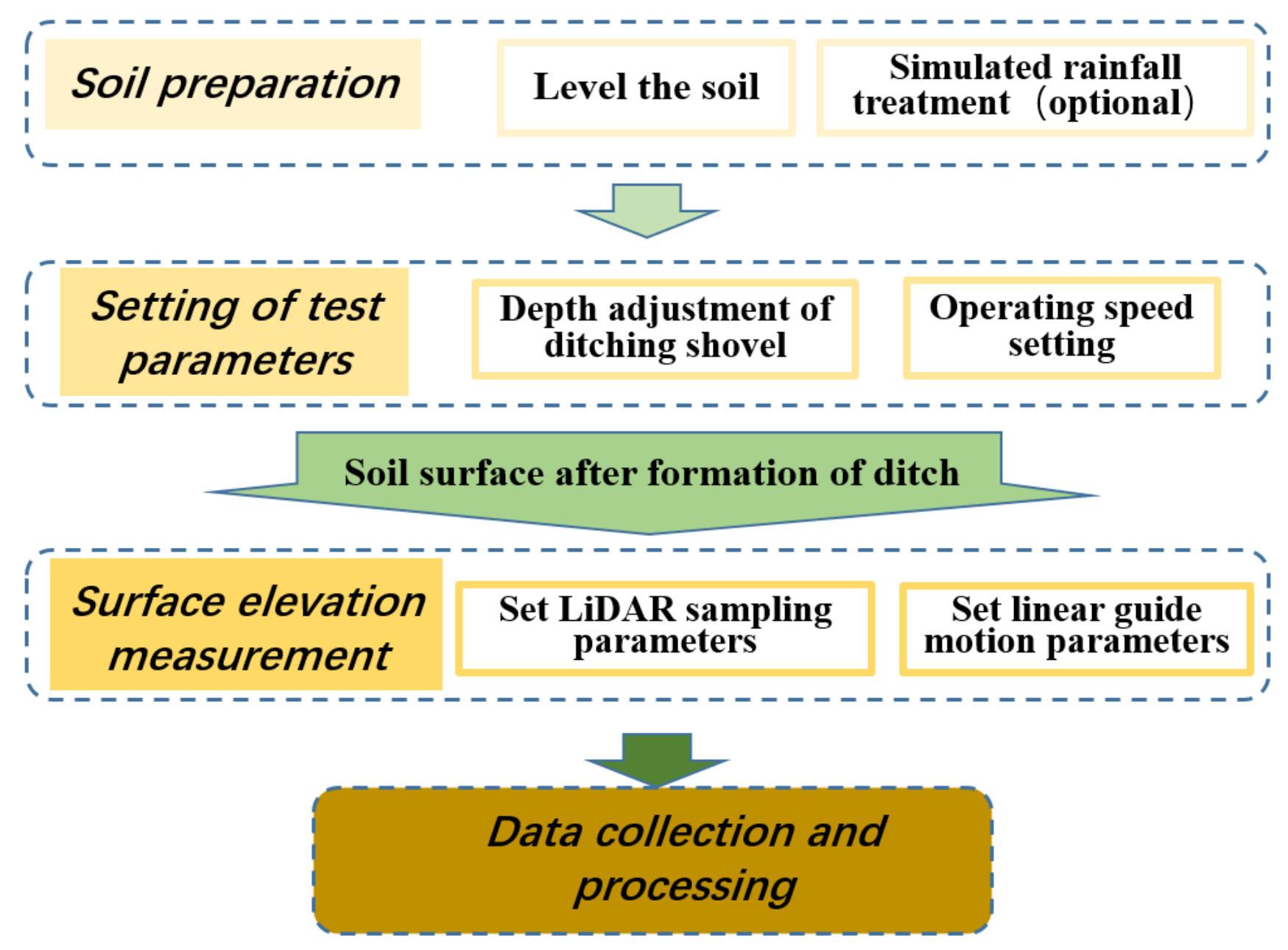
Figure 6.
Relation between the number of wavelet decompositions and the proportion of energy.
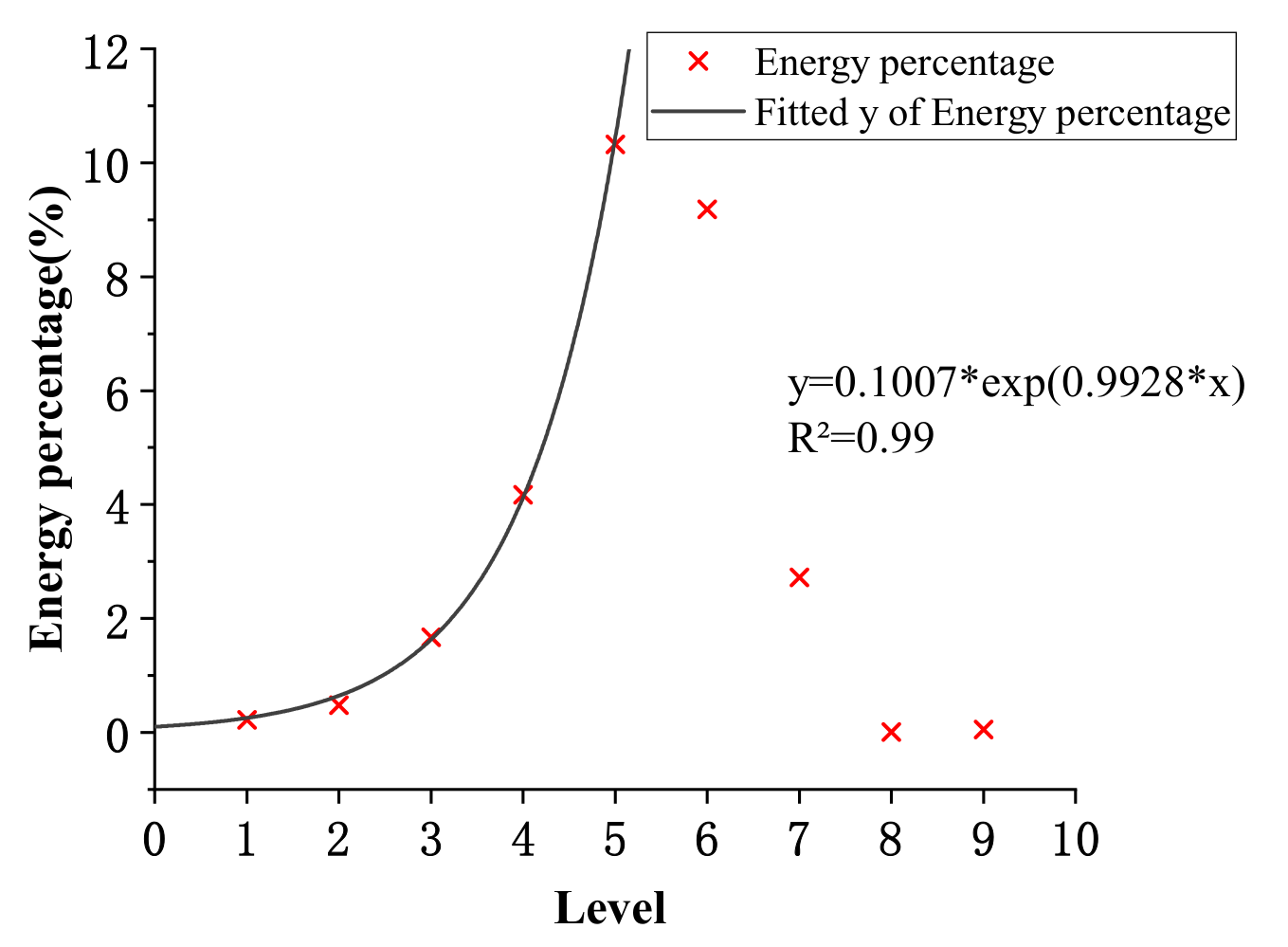
Figure 7.
Digital model of soil surface. (a) Ditching depth of 5 cm. (b) Ditching depth of 8 cm. (c) Ditching depth of 10 cm. (d) Ditching depth of 12 cm.
Figure 7.
Digital model of soil surface. (a) Ditching depth of 5 cm. (b) Ditching depth of 8 cm. (c) Ditching depth of 10 cm. (d) Ditching depth of 12 cm.
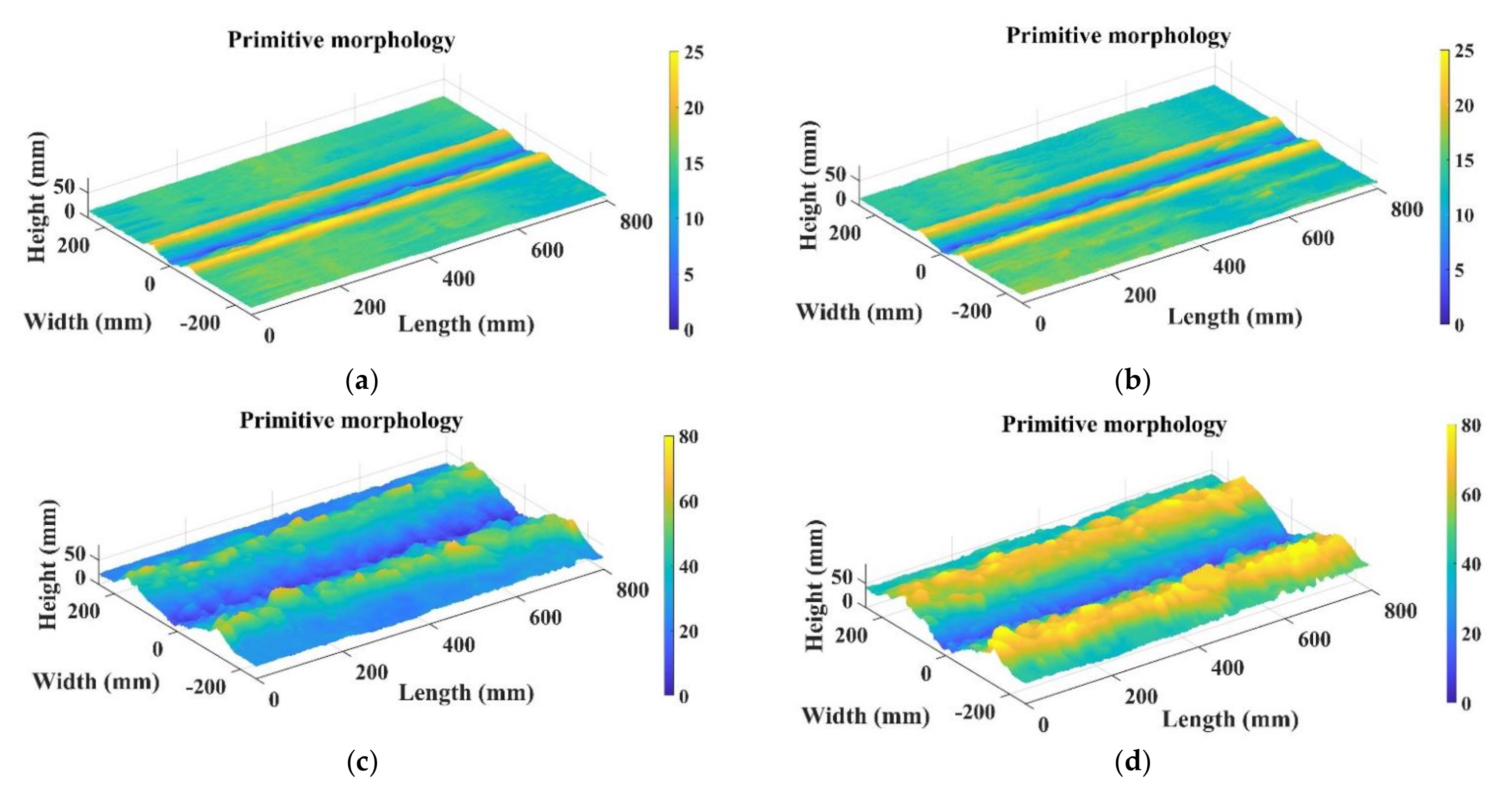
Figure 8.
Wavelet datum and DEM after wavelet transform. (a) Ditching depth of 5 cm. (b) Ditching depth of 8 cm. (c) Ditching depth of 10 cm. (d) Ditching depth of 12 cm.
Figure 8.
Wavelet datum and DEM after wavelet transform. (a) Ditching depth of 5 cm. (b) Ditching depth of 8 cm. (c) Ditching depth of 10 cm. (d) Ditching depth of 12 cm.

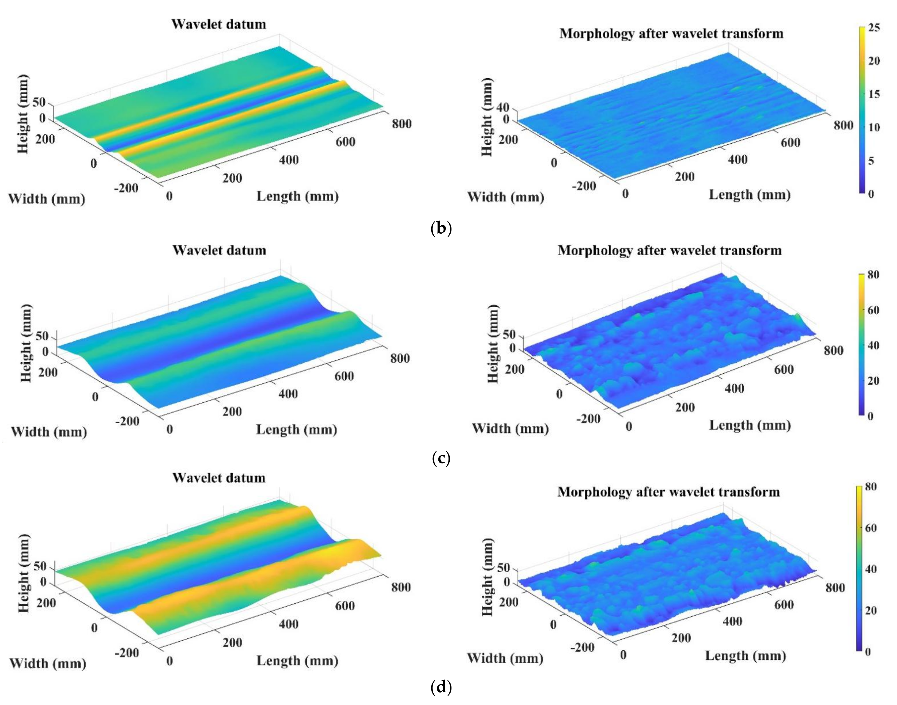
Figure 9.
Cross-sections of digital model and wavelet datum surface under different ditching depths. (a) Ditching depth of 5 cm. (b) Ditching depth of 8 cm. (c) Ditching depth of 10 cm. (d) Ditching depth of 12 cm.
Figure 9.
Cross-sections of digital model and wavelet datum surface under different ditching depths. (a) Ditching depth of 5 cm. (b) Ditching depth of 8 cm. (c) Ditching depth of 10 cm. (d) Ditching depth of 12 cm.

Figure 10.
The roughness of soil surface before and after wavelet transform under different ditching depths and different sampling intervals. (a) Ditching depth of 5 and 8 cm. (b) Ditching depth of 10 and 12 cm.
Figure 10.
The roughness of soil surface before and after wavelet transform under different ditching depths and different sampling intervals. (a) Ditching depth of 5 and 8 cm. (b) Ditching depth of 10 and 12 cm.

Figure 11.
The ACF of the original surface and the soil surface after wavelet transform under different ditching depths. (a) Ditching depth of 5 cm and 8 cm. (b) Ditching depth of 10 cm and 12 cm.
Figure 11.
The ACF of the original surface and the soil surface after wavelet transform under different ditching depths. (a) Ditching depth of 5 cm and 8 cm. (b) Ditching depth of 10 cm and 12 cm.
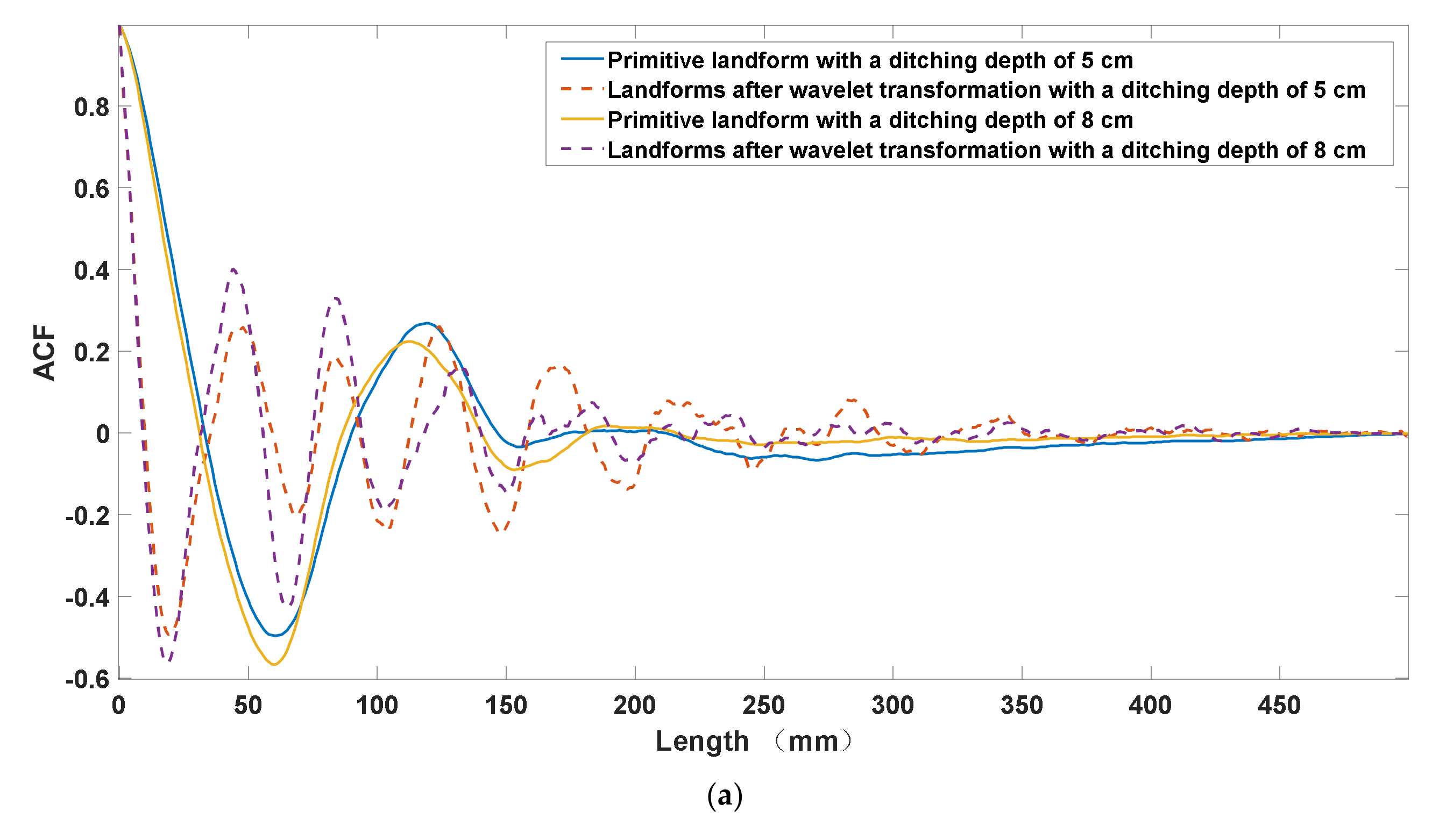
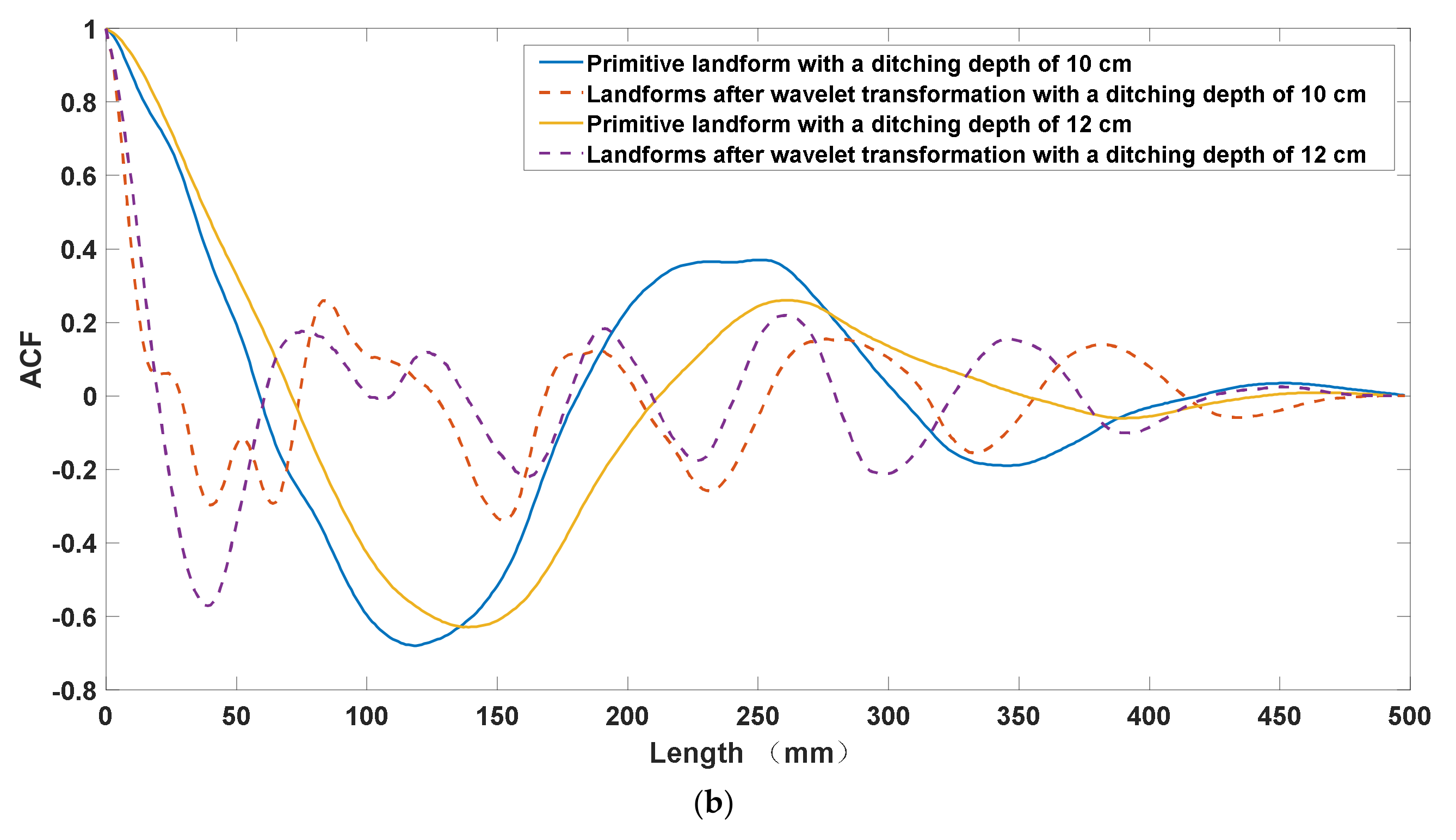
Figure 12.
Concave and convex areas intercepted by 3D digital model of original surface.

Figure 13.
Concave and convex regions at the same position intercepted by the 3D digital model of the soil surface after wavelet transform.
Figure 13.
Concave and convex regions at the same position intercepted by the 3D digital model of the soil surface after wavelet transform.

Table 1.
Comparison of RMSH values of different ditching depths before and after wavelet processing.
Table 1.
Comparison of RMSH values of different ditching depths before and after wavelet processing.
| Ditching Depth/cm | 5 | 8 | 10 | 12 |
|---|---|---|---|---|
| Before wavelet transform/mm | 3.37 | 3.45 | 12.16 | 17.03 |
| After wavelet transform/mm | 1.11 | 1.12 | 4.05 | 4.59 |
| Range of change/% | 203.60 | 208.04 | 200.24 | 271.02 |
Table 2.
Statistical results of original surface and surface CL after wavelet transform with different tillage depth.
Table 2.
Statistical results of original surface and surface CL after wavelet transform with different tillage depth.
| Ditching Depth | Data Type | Cross-Section Serial Number | Average Value | ||||
|---|---|---|---|---|---|---|---|
| 1 | 2 | 3 | 4 | 5 | |||
| 5 cm | Original surface CL | 23.26 | 24.11 | 21.78 | 21.44 | 21.73 | 22.46 |
| Surface CL after wavelet transform | 16.73 | 15.15 | 16.94 | 15.19 | 14.38 | 15.68 | |
| 8 cm | Original surface CL | 23.65 | 23.55 | 23.89 | 23.13 | 22.88 | 23.42 |
| Surface CL after wavelet transform | 15.02 | 15.15 | 14.47 | 16.39 | 17.08 | 15.62 | |
| 10 cm | Original surface CL | 43.11 | 41.73 | 38.78 | 45.09 | 40.76 | 41.89 |
| Surface CL after wavelet transform | 18.94 | 15.73 | 17.78 | 20.76 | 18.80 | 18.40 | |
| 12 cm | Original surface CL | 49.91 | 47.40 | 50.08 | 51.18 | 53.01 | 50.32 |
| Surface CL after wavelet transform | 23.26 | 24.11 | 21.78 | 21.44 | 21.73 | 22.46 | |
Table 3.
The RMSH and CL values of cross-sections in different directions before and after wavelet processing.
Table 3.
The RMSH and CL values of cross-sections in different directions before and after wavelet processing.
| Ditching Depth (cm) | Before Wavelet Transform | After Wavelet Transform | ||||||||||
|---|---|---|---|---|---|---|---|---|---|---|---|---|
| 0° | 45° | 90° | 0° | 45° | 90° | |||||||
| RMSH | CL | RMSH | CL | RMSH | CL | RMSH | CL | RMSH | CL | RMSH | CL | |
| 5 | 3.34 | 21.32 | 3.18 | 21.24 | 1.30 | 48.74 | 1.06 | 6.29 | 1.03 | 6.77 | 1.08 | 32.33 |
| 8 | 3.37 | 19.86 | 3.82 | 24.48 | 0.96 | 20.14 | 1.18 | 7.05 | 1.01 | 6.01 | 0.78 | 10.42 |
| 10 | 13.34 | 38.50 | 13.26 | 39.27 | 5.91 | 32.91 | 4.76 | 17.52 | 3.64 | 12.86 | 4.62 | 17.68 |
| 12 | 17.36 | 51.48 | 15.96 | 48.56 | 5.16 | 26.69 | 4.57 | 15.96 | 4.54 | 12.97 | 3.78 | 13.40 |
Table 4.
Statistical analysis of RR before and after concave and convex wavelet transform.
| Area | RMSH (Mm) | RMSH after Wavelet Transform (Mm) | Amplitude of Change (%) |
|---|---|---|---|
| Convex area | 7.57 | 5.12 | 47.78 |
| Concave area | 5.14 | 3.51 | 46.41 |
Publisher’s Note: MDPI stays neutral with regard to jurisdictional claims in published maps and institutional affiliations. |
© 2022 by the authors. Licensee MDPI, Basel, Switzerland. This article is an open access article distributed under the terms and conditions of the Creative Commons Attribution (CC BY) license (https://creativecommons.org/licenses/by/4.0/).
Share and Cite
MDPI and ACS Style
Liu, L.; Bi, Q.; Zhang, Q.; Tang, J.; Bi, D.; Chen, L. Evaluation Method of Soil Surface Roughness after Ditching Operation Based on Wavelet Transform. Actuators 2022, 11, 87. https://doi.org/10.3390/act11030087
AMA Style
Liu L, Bi Q, Zhang Q, Tang J, Bi D, Chen L. Evaluation Method of Soil Surface Roughness after Ditching Operation Based on Wavelet Transform. Actuators. 2022; 11(3):87. https://doi.org/10.3390/act11030087
Chicago/Turabian StyleLiu, Lichao, Quanpeng Bi, Qianwei Zhang, Junjie Tang, Dawei Bi, and Liqing Chen. 2022. "Evaluation Method of Soil Surface Roughness after Ditching Operation Based on Wavelet Transform" Actuators 11, no. 3: 87. https://doi.org/10.3390/act11030087
Note that from the first issue of 2016, this journal uses article numbers instead of page numbers. See further details here.