Research on the Identification of Tyre-Road Peak Friction Coefficient under Full Slip Rate Range Based on Normalized Tyre Model

Abstract

The accurate estimation of the tyre-road peak friction coefficient is the key basis for the normal operation of the vehicle active safety control system. The estimation algorithm needs to be able to adapt to various conditions encountered in the actual driving process of the vehicle and obtain the estimation results timely and accurately. Therefore, a new normalized strategy is proposed in this paper. The core is the equal ratio between the peak friction coefficient and the utilization friction coefficient between adjacent typical roads. This strategy can establish the direct connection (normalization) between tyre force and tyre-road peak friction coefficient through most tyre models in the field of vehicle dynamics and accomplish estimation by combining with the filtering algorithm. In addition, most of the vehicle dynamic estimation algorithms are limited by road excitation, and it is difficult to obtain satisfactory estimation results. This strategy can greatly reduce the system error caused by insufficient road excitation (slip rate is not 0.15–0.20) and improve the applicability of the estimation algorithm to the actual driving process of the vehicle. Finally, the magic formula (MF) tyre model is selected to describe the tyre characteristics after treatment of the normalized strategy; the tyre-road peak friction coefficient is estimated by combining the extended Kalman filter and vehicle dynamics model. Satisfactory estimation results are obtained in both simulation and real vehicle tests, which verifies the effectiveness of the proposed normalized strategy.

1. Introduction

The tyre-road friction coefficient can describe the friction between the tyre and the road, which is very important for vehicle active safety control technology. The accurate estimation of the tyre-road friction coefficient helps to control vehicle driving performance, reduce slippage, and improve vehicle-handling stability. A large number of studies on vehicle stability have clearly put forward the use of the tyre-road friction coefficient to promote the improvement of vehicle safety control systems [1,2,3]. Therefore, the real-time and accurate estimation of the tyre-road friction coefficient is of great significance to improve the performance of vehicle control systems, such as the anti-lock braking system (ABS), electronic stability control (ESC), and active yaw control system (AYC) [2,4,5,6].

In recent years, scholars have conducted extensive research on the estimation method of the tyre-road friction coefficient and basically formed two kinds of estimation methods [7,8,9]: experiment-based and model-based.

The experiment-based method mainly measures the relevant signals (such as road surface morphology, tyre deformation, and noise) directly by sensors and establishes the corresponding relationships to obtain the tyre-road friction coefficient [7]. Among them, Leng B. et al. [10] accomplished road recognition and classification by extracting road color and texture features; Hong S. et al. [11] placed piezoelectric sensors inside the tyre to measure the lateral deflection of the tyre section and to estimate the tyre-road friction coefficient; J. Alonso et al. [12] used acoustic sensors to select and extract tyre noise to accomplish road recognition. The advantage of this kind of method is that it has a wide range of identification and a predictive effect [7,13]. However, its effectiveness is easily affected by the environment, and the sensors that need to be matched are relatively expensive [14], which is difficult for large-scale promotion.

The model-based estimation method only uses the common low-cost sensors of vehicles to measure or estimate the dynamic response change on the wheel or car body caused by the change in the tyre-road friction coefficient and then calculates the tyre-road friction coefficient [7]. Due to the wide applicability and high precision of this kind of algorithm, scholars have conducted a large body of research, which can be roughly divided into four kinds. The first is the tyre-road friction coefficient estimation method based on the slip-slope relationship. Gustafsson F. [15,16] proposed a tyre-road friction coefficient estimation method based on slip-slope, which has high accuracy only when the slip rate is less than 0.05. Wang J. et al. [17] improved the literature [15,16] and accomplished the coefficient identification of large-scale, slip rate driving conditions, but the estimation results cannot be updated at very low slip rates. The second is the estimation method based on nonlinear formula fitting. Germann S. et al. [18] fitted the nonlinear function based on the linear function, and Castro R.D. et al. [19] fitted the nonlinear equation based on the feedforward neural network (FFNN), both combined with the recursive least squares estimator to accomplish the online estimation of the tyre-road friction coefficient. This method is simple in principle, but it is difficult to guarantee the real-time performance. The third is the estimation method based on road state characteristic factors. Wang B. et al. [20] accomplished road recognition by constructing an eigenvalue that can represent typical road characteristic parameters. The method covers almost all the roads where cars normally travel and requires less sensor signals, but it is limited to straight braking conditions.

The fourth is the estimation method of the tyre-road friction coefficient based on tyre model, which is divided into two categories. The first category is based on the relationship between the tyre mechanical properties and the tyre-road friction coefficient, the slip rate in tyre model. By observing the tyre mechanical state (such as longitudinal force and lateral force), the parameters characterizing the tyre-road friction coefficient in tyre models (such as Dugoff [21,22], LuGre [23,24], Brush [25,26]) are calculated. In the second category, the tyre force is normalized based on the tyre model (such as Dugoff [27,28], Hsri [29], MF [30,31], Uni-tyre [32]), and the tyre-road friction coefficient is separated from the normalized force, which is suitable for establishing the system equation. The tyre-road friction coefficient is estimated by combining the filtering algorithm or iterative algorithm. This method based on the tyre model is called the normalized method according to the following reason. Since there are a large number of mature tyre model studies that can be referred to, different tyre models can be used to study different tyre dynamics fields, which offers great potential for the normalization methods based on tyre model. However, the estimation method based on a certain tyre model is limited in terms of accuracy, adaptability, and real-time performance.

The problems in the above model-based research are: most are based on longitudinal or lateral studies, with little regard to longitudinal- and lateral-coupling processes; most only consider a certain segment of the slip rate interval [0, 1]; they do not consider the corresponding relationship between the slip rate and the estimated tyre-road friction coefficient; the robustness and accuracy of the estimation algorithm cannot be guaranteed; as some novel algorithms only rely on Simulink, CarSim, and other simulation software to verify and do not use real vehicle verification, the actual feasibility is not verified; although some estimation algorithms have high estimation accuracy, they have large amounts of calculations and cannot guarantee real-time performance.

It can be seen from the above content that the characteristics of the estimation algorithm should be simple and practical and should have strong robustness, fast convergence, and strong incentive sensitivity. In the model-based estimation method, the principle of the estimation method based on the tyre model is easy to understand, the estimation accuracy is controllable, and the plasticity is strong. Among them, the normalization method based on a tyre model is simple and has a standard estimation process, which has the potential to apply to use most of the tyre models in the field of vehicle dynamics and makes this method most likely to have the above four excellent characteristics at the same time.

However, the performance of the normalization method based on a tyre model depends on the type of tyre model, and the algorithm can achieve the best performance by matching the high-precision tyre model in the research field. However, not all tyre models can be directly used for normalization. Usually, the more accurate the tyre model is, the more complex it is. Few simple tyre models can accurately reproduce the friction performance of the tyre-road interface while maintaining a simple form [33]. Therefore, a high precision tyre model is difficult to be used in this method.

In view of the difficulties faced by the normalized method based on tyre model, a new normalized strategy is proposed in this paper. This strategy establishes a direct connection between the tyre force output from the tyre model and the tyre-road peak friction coefficient according to the equal ratio relationship between tyre-road peak friction coefficient and the utilization of the friction coefficient on the adjacent typical roads. Normalization is achieved by introducing parameters from outside to avoid complex internal functions. The normalized tyre model is combined with the filtering algorithm and vehicle dynamics model to estimate the tyre-road peak friction coefficient. The normalized strategy can be applied to most tyre models in the field of vehicle dynamics, which means that almost all tyre models can be used to estimate the tyre-road peak friction coefficient. Different tyre models have high-fitting accuracy in different fields, which greatly expands the application scope of the tyre-road friction coefficient estimation algorithm based on tyre model.

In addition, most estimation algorithms can obtain accurate results only when the slip rate is within optimal range [0.15, 0.2], but the actual value of slip rate rarely reaches the optimal level in the vehicle-driving process. Additionally, at the optimal slip ratio stage, the road excitation on the tyre is too intense, which will negatively affect the vehicle-handling stability and comfort [5]. The system error in the non-optimal slip rate stage can be avoided using the equal ratio relationship. Therefore, in full slip rate range conditions, this algorithm can obtain accurate estimation results, and the robustness of the algorithm and high sensitivity to road excitation are ensured.

Finally, the classic MF tyre model is selected as the representative of complex tyre models. Combining the vehicle dynamics model and the extended Kalman filter, the tyre-road peak friction coefficient is estimated. The above algorithm is verified in simulation and in a real vehicle test.

The other parts are set as follows: the first part establishes the vehicle dynamics model; the second part mainly introduces the normalized strategy; the third part introduces the extended Kalman filter; the fourth and fifth parts are simulation and experimental verification; the sixth part is the conclusion.

2. Establish Vehicle Dynamics Model

The 3 DOF vehicle dynamics model is established, as shown in Figure 1.

The following motion differential equations are established.

Longitudinal equation:

$$m_z({\dot{v}}_x-v_y\gamma )=F_{xfl}\cos {\delta }_f-F_{yfl}\sin {\delta }_f+F_{xfr}\cos {\delta }_f-F_{yfr}\sin {\delta }_f+F_{xrl}+F_{xrr}$$

(1)

Lateral equation:

$$m_z({\dot{v}}_y+v_x\gamma )=F_{xfl}\sin {\delta }_f+F_{yfl}\cos {\delta }_f+F_{xfr}\sin {\delta }_f+F_{yfr}\cos {\delta }_f+F_{yrl}+F_{yrr}$$

(2)

Yaw equation:

$$\dot{\gamma }{I}_z=a(F_{xfl}\sin {\delta }_f+F_{yfl}\cos {\delta }_f+F_{xfr}\sin {\delta }_f+F_{yfr}\cos {\delta }_f)+\frac{T}{2}(F_{xrr}+F_{xfr}\cos {\delta }_f-F_{yfr}\sin {\delta }_f)-\frac{T}{2}(F_{xfl}\cos {\delta }_f-F_{yfl}\sin {\delta }_f+F_{xrl})-(F_{yrl}+F_{yrr})b$$

(3)

The load on each wheel can be expressed as:

$$F_{zfl}=\frac{b}{2L}{m}_{z}g-\frac{b{h}_g}{LT}{m}_b{a}_y-\frac{m_b{a}_x{h}_g}{2L}+k_{\psi }{\psi }_b$$

(4)

$$F_{zfr}=\frac{b}{2L}{m}_{z}g+\frac{b{h}_g}{LT}{m}_b{a}_y-\frac{m_b{a}_x{h}_g}{2L}+k_{\psi }{\psi }_b$$

(5)

$$F_{zrl}=\frac{a}{2L}{m}_{z}g-\frac{a{h}_g}{LT}{m}_b{a}_y+\frac{m_b{a}_x{h}_g}{2L}+k_{\psi }{\psi }_b$$

(6)

$$F_{zrr}=\frac{a}{2L}{m}_{z}g+\frac{a{h}_g}{LT}{m}_b{a}_y+\frac{m_b{a}_x{h}_g}{2L}+k_{\psi }{\psi }_b$$

(7)

where $F_{xfl}, F_{xfr}, F_{xrl}, F_{xrr}, F_{yfl}, F_{yfr}, F_{yrl}, \mathrm{and}{F}_{yrr}$ are the longitudinal and lateral forces of the four wheels, respectively; $v_x \mathrm{and}{v}_y$ are the longitudinal and lateral velocities of the vehicle centroid, respectively; $\gamma , {\psi }_b, \mathrm{and}{\delta }_f$ are the yaw rate, roll angle, and front wheel angle, respectively; g is $9.8$ m/s², $a_x \mathrm{and} a_y$ are the longitudinal and lateral accelerations of the vehicle centroid, respectively. The main parameters of the vehicle dynamics model are shown in

Table 1. The main parameters of the test vehicle.

Symbol	Value	Notes
mz	880 kg	Vehicle mass
mb	788 kg	Sprung mass
L	2.040 m	Wheel base
a	1.145 m	Distance from centroid to front axle
b	0.895 m	Distance from centroid to rear axle
hg	0.54 m	Centroid height
T	1.3 m	Wheel track width
Iz	832.3 kg·m2	Moment of inertia about the z-axis
KΨ	25,041 N/rad	Tyre slip angle stiffness

.

3. Normalized Strategy

3.1. Estimation Algorithm Process

The overall estimation algorithm process is shown in Figure 2.

The sensor signals from CarSim or real vehicle tests are processed to obtain the required parameters. Based on the Kiencke tyre model [34], the equal ratio relationship is proposed. Normalization of tyre model can be accomplished by this relationship. The normalized strategy framework is shown in Figure 3. The MF tyre model [35,36,37] is selected as the representative of high precision and high complexity tyre model. The normalized tyre model is matched with the vehicle dynamics model, and the estimated value of the tyre-road peak friction coefficient is obtained by the extended Kalman filter [38,39].

3.2. Construction of Normalized Strategy

3.2.1. Kiencke Tyre Model

The Kiencke tyre model optimized the Buckhardt tyre model [40], as shown in Equation (8).

$${\mu }_{Res}(s_{Res})=(c_1(1-e^{-c_2{s}_{Res}})-c_3{s}_{Res})\cdot e^{-c_4\cdot s_{Res}\cdot v_c}\cdot (1-c_5{F}_Z^2)$$

(8)

where ${\mu }_{Res}$ is the tyre-road utilization friction coefficient, $s_{Res}$ is slip rate, and $v_c$ is the speed of the vehicle center of gravity. $F_z$ is the vertical load on the vehicle. $c_1$, $c_2$, and $c_3$ change with road conditions. The parameter values of six typical roads are given in

Table 2. $c_2$ and $c_3$ fitting coefficient.

Road Surface Type	c1	c2	c3
Dry asphalt	1.2801	23.99	0.52
Wet asphalt	0.857	33.822	0.347
Cement	1.1973	25.168	0.5373
Wet pebbles	0.4004	33.7080	0.1204
Ice	0.05	306.39	0
Snow	0.1946	94.129	0.0646

[40]. The value of $c_4$ is between $0.002$ s/m and $0.004$ s/m, and the value of $c_5$ is $0.00015$ (1/kN)² [34].

3.2.2. Similarity Analysis

According to the Kiencke tyre model, the relationship between the tyre-road utilization friction coefficient and the slip rate on the typical roads can be obtained, as shown in Figure 4.

It can be seen from Figure 4 that under six typical roads, the change trend of the curve between the tyre-road utilization friction coefficient and slip rate is similar, especially between adjacent typical roads, such as asphalt and cement and wet pebbles and snow. Therefore, the relationship between the tyre-road utilization friction coefficient and the peak friction coefficient can be expressed as [41]:

$$\frac{{\mu }_{\mathrm{Re}sg}}{{\mu }_{\mathrm{R}\max g}}=\frac{{\mu }_{\mathrm{Re}sh}}{{\mu }_{\mathrm{R}\max h}}$$

(9)

assuming that road g and h are adjacent, and they are the target road and the adjacent road, respectively. ${\mu }_{\mathrm{Re}sg}$ and ${\mu }_{\mathrm{Re}sh}$ are the tyre-road utilization friction coefficients of road g and h, respectively. ${\mu }_{\mathrm{R}\max g}$ and ${\mu }_{\mathrm{R}\max h}$ are the tyre-road peak friction coefficients of road g and h, respectively.

3.3. Tyre Model

The tyre force driving on the known road can be obtained by the tyre model. There are many tyre models in the field of vehicle dynamics, such as Dugoff, MF, LuGre, and Uni-Tyre. Therefore, in the control process, we can select the tyre model with the highest accuracy according to the tyre dynamic field studied.

The MF tyre model is widely used in vehicle dynamics simulation and analysis due to its high simulation accuracy and wide application range [7]. Because of its complex form and numerous and interrelated parameters, the MF tyre model is difficult to use directly for the normalized estimation algorithm.

To verify the normalized strategy, this paper will take the MF tyre model as an example to study the estimation of the tyre-road peak friction coefficient.

3.3.1. MF Tyre Model

In a single condition, the general expression of the longitudinal tyre force, $F_{x0}$, and the lateral tyre force, $F_{y0}$, is

$$F_{x0}=D_x\sin \{C_x{\tan }^{-1}[B_x{\kappa }_x-E_x(B_x{\kappa }_x-{\tan }^{-1}(B_x{\kappa }_x))]\}+S_{Vx}$$

(10)

$$F_{y0}=D_y\sin \{C_y{\tan }^{-1}[B_y{\alpha }_y-E_y(B_y{\alpha }_y-{\tan }^{-1}(B_y{\alpha }_y))]\}+S_{Vy}$$

(11)

Under combined conditions, the longitudinal tyre force and lateral tyre force can be expressed as

$$\{\begin{array}{l}{F}_x=\frac{\left|{\sigma }_x\right|}{\sigma }{F}_{x0}\\ F_y=\frac{\left|{\sigma }_y\right|}{\sigma }{F}_{y0}\end{array}$$

(12)

The factors can be expressed as

$$\{\begin{array}{l}{\sigma }_x=\frac{\kappa }{1+\kappa }\\ {\sigma }_y=\frac{\tan \alpha }{1+\kappa }\\ \sigma =\sqrt{{\sigma }_x^2+{\sigma }_x^2}\end{array}$$

(13)

Longitudinal slip rate can be expressed as

$${\kappa }_x=\frac{\omega r_e-v_{tx}}{v_{tx}}$$

(14)

where $r_e$ is the effective rolling radius of the wheel.

The tyre sideslip angle can be expressed as

$$\alpha =\delta -{\tan }^{-1}(\frac{v_{ty}}{\left|v_{tx}\right|})$$

(15)

where $v_{tx}$ is the longitudinal wheel speed and $v_{ty}$ is lateral wheel speed. For other parameters, see Appendix A.

3.3.2. Normalization of Tyre Model

Under pure longitudinal or pure lateral conditions, the MF tyre model can be expressed as

$$F=D\sin \{C{\tan }^{-1}[B\kappa -E(B\kappa -{\tan }^{-1}(B\kappa ))]\}+S_v$$

(16)

Tyre force can be expressed as [36]

$$F={\mu }_{R\max g}{F}_z$$

(17)

Combined with Equation (9), it can be extended to adjacent typical roads with different friction coefficients [40], which is

$$\frac{F_g}{{\mu }_{R\max g}}=\frac{F_h}{{\mu }_{R\max h}}$$

(18)

$F_g$ is the tyre force when the vehicle runs on the target road. $F_h$ is the tyre force when the vehicle runs on the adjacent road.

Equation (18) is simply transformed to

$$F_g=\frac{{\mu }_{R\max g}{F}_h}{{\mu }_{R\max h}}$$

(19)

Among them, ${\mu }_{R\max g}$ is the tyre-road peak friction coefficient which is to be identified.

In summary, for pure longitudinal conditions and pure lateral conditions, the tyre force can be expressed as:

$$F_{xg}=\frac{{\mu }_{R\max g}{F}_{xh}}{{\mu }_{R\max h}}$$

(20)

$$F_{yg}=\frac{{\mu }_{R\max g}{F}_{yh}}{{\mu }_{R\max h}}$$

(21)

where $F_{xg}$ is the tyre force when the vehicle is in the pure longitudinal condition and runs on the target road. $F_{\mathrm{y}g}$ is the tyre force when the vehicle is in the pure lateral condition and runs on the target road.

According to Equations (10)–(12), the tyre force in the combined conditions can be expressed as

$$F_x={\mu }_{R\max g}{F}_x^0$$

(22)

$$F_x^0=\frac{\left|{\sigma }_x\right|}{{\mu }_{R\max h}\sigma }\{D_x\sin [C_x{\tan }^{-1}[B_x{\kappa }_x-E_x(B_x\kappa -{\tan }^{-1}(B_x{\kappa }_x))]]+S_{Vx}\}$$

(23)

$$F_y={\mu }_{R\max g}{F}_y^0$$

(24)

$$F_y^0=\frac{\left|{\sigma }_y\right|}{{\mu }_{{}_{R\max h}}\sigma }\{D_y\sin [C_y{\tan }^{-1}[B_y{\alpha }_y-E_y(B_y{\alpha }_y-{\tan }^{-1}(B_y{\alpha }_y))]]+S_{Vy}\}$$

(25)

where $F_x^0$ and $F_y^0$ are the longitudinal and lateral normalized forces, respectively, independent of the tyre-road peak friction coefficient to be identified.

3.3.3. Establish System Equation

The following equations are used to estimate the tyre-road peak friction coefficient and are according to Equations (1)–(3), (22) and (24)

$${\dot{v}}_x-v_y\gamma ={\mu }_{fl}(\frac{F_{{}_{xfl}}^0\cos {\delta }_f}{m_z}-\frac{F_{{}_{yfl}}^0\sin {\delta }_f}{m_z})+{\mu }_{rl}\frac{F_{{}_{xrl}}^0}{m_z}+{\mu }_{fr}(\frac{F_{{}_{xfr}}^0\cos {\delta }_f}{m_z}-\frac{F_{{}_{yfr}}^0\sin {\delta }_f}{m_z})+{\mu }_{rr}\frac{F_{{}_{xrr}}^0}{m_z}$$

(26)

$${\dot{v}}_y+v_x\gamma ={\mu }_{rl}\frac{F_{{}_{yrl}}^0}{m_z}+{\mu }_{rr}\frac{F_{{}_{yrr}}^0}{m_z}+{\mu }_{fl}(\frac{F_{{}_{xfl}}^0\sin {\delta }_f}{m_z}+\frac{F_{{}_{yfl}}^0\cos {\delta }_f}{m_z})+{\mu }_{fr}(\frac{F_{{}_{xfr}}^0\sin {\delta }_f}{m_z}+\frac{F_{{}_{yfr}}^0\cos {\delta }_f}{m_z})$$

(27)

$$\begin{array}{l}\dot{\gamma }={\mu }_{fl}(\frac{a}{I_z}{F}_{{}_{xfl}}^0\sin {\delta }_f-\frac{T}{2I_z}{F}_{{}_{xfl}}^0\cos {\delta }_f+\frac{a}{I_z}{F}_{{}_{yfl}}^0\cos {\delta }_f+\frac{T}{2I_z}{F}_{{}_{yfl}}^0\sin {\delta }_f)\\ +{\mu }_{fr}(\frac{a}{I_z}{F}_{{}_{xfr}}^0\sin {\delta }_f+\frac{T}{2I_z}{F}_{{}_{xfr}}^0\cos {\delta }_f+\frac{a}{I_z}{F}_{{}_{yfr}}^0\cos {\delta }_f-\frac{T}{2I_z}{F}_{{}_{yfr}}^0\sin {\delta }_f)\\ -{\mu }_{rl}(\frac{T}{2I_z}{F}_{{}_{xrl}}^0+\frac{b}{I_z}{F}_{{}_{yrl}}^0)+{\mu }_{rr}(\frac{T}{2I_z}{F}_{{}_{xrr}}^0-\frac{b}{I_z}{F}_{{}_{yrr}}^0)\end{array}$$

(28)

The state equation and measurement equation can be obtained by Equations (26)–(28). The state equation is:

$$\left(\begin{array}{c}{\mu }_{fl}(n+1)\\ {\mu }_{fr}(n+1)\\ {\mu }_{rl}(n+1)\\ {\mu }_{rr}(n+1)\end{array}\right)=\left(\begin{array}{cccc}1& 0& 0& 0\\ 0& 1& 0& 0\\ 0& 0& 1& 0\\ 0& 0& 0& 1\end{array}\right)\left(\begin{array}{l}{\mu }_{fl}(n)\\ {\mu }_{fr}(n)\\ {\mu }_{rl}(n)\\ {\mu }_{rr}(n)\end{array}\right)+w(t)$$

(29)

The measurement equation can be expressed as:

$$\left(\begin{array}{c}({\dot{v}}_x-v_y\gamma )\\ {\dot{v}}_y+v_x\gamma \\ \dot{\gamma }\end{array}\right)=\left(\begin{array}{cccc}H(1,1)& H(1,2)& H(1,3)& H(1,4)\\ H(2,1)& H(2,2)& H(2,3)& H(2,4)\\ H(3,1)& H(3,2)& H(3,3)& H(3,4)\end{array}\right)\left(\begin{array}{l}{\mu }_{fl}\\ {\mu }_{fr}\\ {\mu }_{rl}\\ {\mu }_{rr}\end{array}\right)+v(t)$$

(30)

$$\{\begin{array}{l}H(1,1)=\frac{F_{{}_{xfl}}^0\cos {\delta }_f}{m_z}-\frac{F_{{}_{yfl}}^0\sin {\delta }_f}{m_z}\\ H(1,2)=\frac{F_{{}_{xfr}}^0\cos {\delta }_f}{m_z}-\frac{F_{{}_{yfr}}^0\sin {\delta }_f}{m_z}\\ H(1,3)=\frac{F_{{}_{xrl}}^0}{m_z},H(1,4)=\frac{F_{{}_{xrr}}^0}{m_z}\\ H(2,1)=\frac{F_{{}_{xfl}}^0\sin {\delta }_f}{m_z}+\frac{F_{{}_{yfl}}^0\cos {\delta }_f}{m_z}\\ H(2,2)=\frac{F_{{}_{xfr}}^0\sin {\delta }_f}{m_z}+\frac{F_{{}_{yfr}}^0\cos {\delta }_f}{m_z}\\ H(2,3)=\frac{F_{{}_{yrl}}^0}{m_z},H(2,4)=\frac{F_{{}_{yrr}}^0}{m_z}\\ H(3,1)=\frac{a}{I_z}{F}_{{}_{xfl}}^0\sin {\delta }_f-\frac{T}{2I_z}{F}_{{}_{xfl}}^0\cos {\delta }_f+\frac{a}{I_z}{F}_{{}_{yfl}}^0\cos {\delta }_f+\frac{T}{2I_z}{F}_{{}_{yfl}}^0\sin {\delta }_f\\ H(3,2)=\frac{a}{I_z}{F}_{{}_{xfr}}^0\sin {\delta }_f+\frac{T}{2I_z}{F}_{{}_{xfr}}^0\cos {\delta }_f+\frac{a}{I_z}{F}_{{}_{yfr}}^0\cos {\delta }_f-\frac{T}{2I_z}{F}_{{}_{yfr}}^0\sin {\delta }_f\\ H(3,3)=-\frac{T}{2I_z}{F}_{{}_{xrl}}^0-\frac{b}{I_z}{F}_{{}_{yrl}}^0\\ H(3,4)=\frac{T}{2I_z}{F}_{{}_{xrr}}^0-\frac{b}{I_z}{F}_{{}_{yrr}}^0\end{array}$$

(31)

Among them, ${\mu }_{xij}(ij=fl,fr,rl,rr)$ represents the peak friction coefficient between the four tyres and the target road, and the random variables, $w(t)$ and $v(t)$, are process noise and measurement noise, respectively.

3.4. Determination of Adjacent Road

According to the existing research and experimental data [2], the tyre-road friction coefficient in Figure 4 is higher than the actual value. However, this does not affect the equal ratio relationship between the tyre-road utilization friction coefficient and the peak friction coefficient.

In the simulation part, the tyre-road peak friction coefficient is set to 0.85 and 0.9, respectively. The real vehicle test road is dry asphalt road; thus, the adjacent road is cement road.

4. EKF Estimation Algorithm

The extended Kalman filter estimation process [38] is shown in Figure 5.

The initial value in the filtering process can be expressed as the measurement noise covariance, $R=0.03\times I_{3\times 3}$, and the process noise covariance is $P=0.01\times I_{4\times 4}$, the initial covariance matrix is $P_0=0.02\times I_{4\times 4}$, and the initial estimate states matrix is ${\mu }_{\mathrm{R}\max }={[0,0,0,0]}^T$.

The systematic equations are illustrated in Section 3.3.3.

5. Simulation Analysis and Verification

In this paper, Carsim and Matlab/Simulink are used for the simulation of the linear-braking condition and the curve-braking condition.

5.1. Simulation on High Adhesion Road

5.1.1. Linear-Braking Condition

The tyre-road peak friction coefficient is set to 0.85, and the initial velocity is 120 km/h. The simulation [42] results, shown in Figure 6a–c, are based on the four wheels of the car on the road with the same friction coefficient road, while considering the length of the article and taking the right front wheel as an example.

It can be seen from Figure 6a–c that the braking deceleration is close to 5.5 m/s². The slip rate of the right front wheel remains around 0.08, which is not enough to reach the range [0.15, 0.20] of slip rate corresponding to sufficient road excitation. However, the tyre-road peak friction coefficient converges to 0.85 before 0.4 s, and the overall situation is stable.

5.1.2. Curve-Braking Combined Condition

The annular road [43] with 33 m radius is set, the tyre-road peak friction coefficient is 0.9, and the initial speed is 60 km/h. Taking the right front wheel as an example, the simulation results are shown in Figure 6d–h.

It can be seen from Figure 6d–h that the maximum steering wheel angle is close to 170 degrees, the maximum braking deceleration is close to 4 m/s², and the slip rate is close to [0.15–0.20] at 0.2–1.4 s. At this time, the road excitation is close to sufficient. Under this condition, the estimated value of the tyre-road peak friction coefficient converges to 0.9 at about 0.2 s, remains stable to 1 s, then decreases to 0.87, lasts to 2.3 s, and then rises to 0.93. The overall value is maintained at about 0.9, and the error is maintained within [−0.04, 0.04].

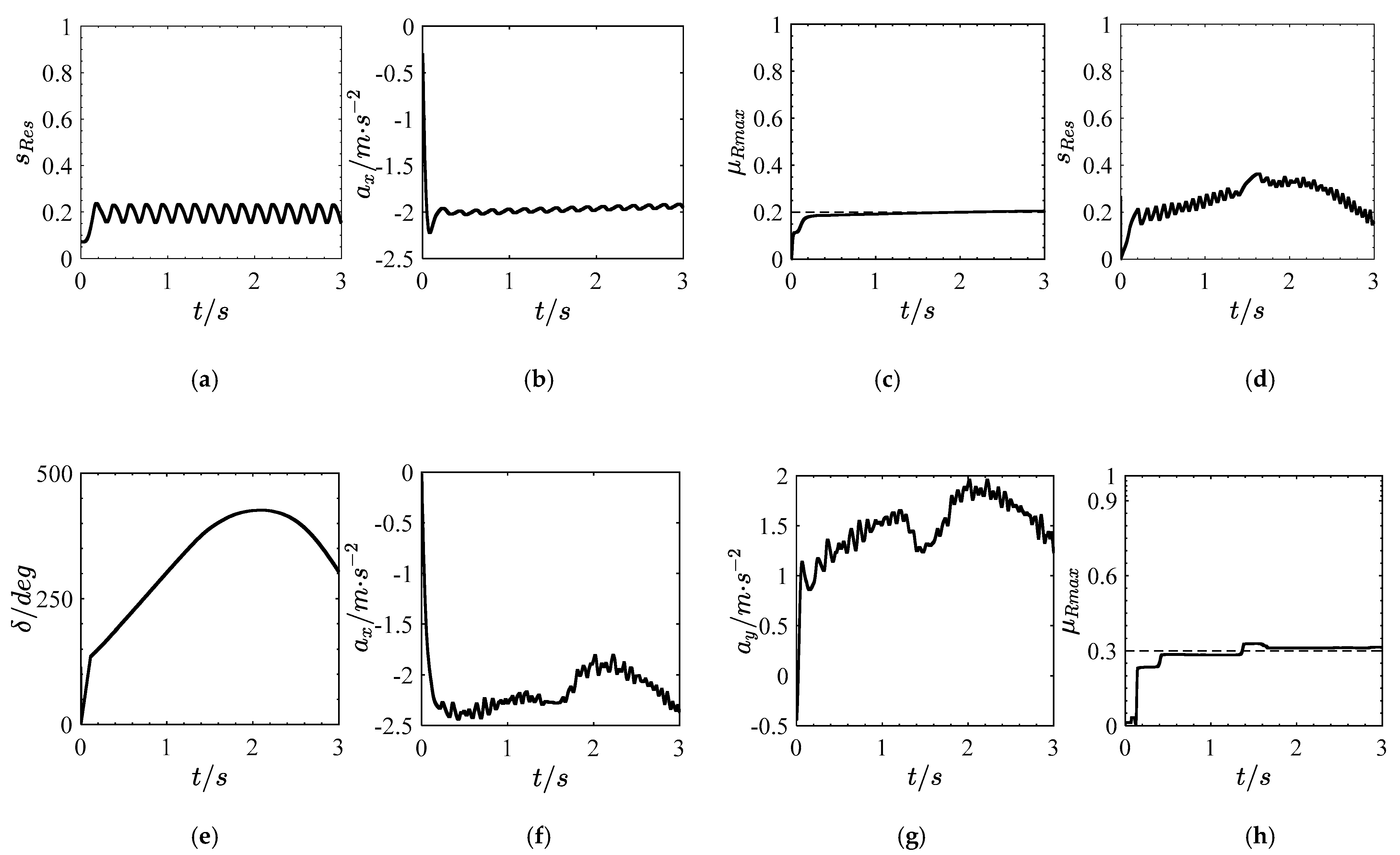
5.2. Simulation on Low Adhesion Road

5.2.1. Linear-Braking Condition

The tyre-road peak friction coefficient is set to 0.2, and the initial velocity is 120 km/h. Taking the right front wheel as an example, the simulation results are shown in Figure 7a–c.

It can be seen from Figure 7a–c that the slip rate remains in [0.15, 0.24], which shows the road excitation is sufficient relatively. The braking deceleration is close to 2 m/s². Additionally, the tyre-road peak friction coefficient converges to 0.2 at about 0.2 s and then remains basically stable.

5.2.2. Curve-Braking Combined Condition

The tyre-road peak friction coefficient is set to 0.3. Under turning conditions on low adhesion road, the initial speed is reduced to 35 km/h. Taking the right front wheel as an example, the simulation results are shown in Figure 7d–h.

It can be seen from Figure 7d–h that the slip rate fluctuates between [0.15 and 0.36] and mostly lies outside the optimum interval, which indicates the road excitation level is insufficient. The maximum longitudinal deceleration can reach 2.5 m/s², and the maximum lateral acceleration can reach 2 m/s². The estimation result converges to 0.3 before 0.45 s, and the estimation error is maintained within [−0.05, 0.05].

6. Test Verification

6.1. Calibration Test of Tyre-Road Peak Friction Coefficient

The BM-III pendulum friction coefficient tester [44] was used to calibrate the tyre-road peak friction coefficient of the test asphalt road surface. The test road is a 100 m straight road; the test results are shown in Figure 8.

Figure 8 shows that the actual value range of the tyre-road peak friction coefficient on the measured dry asphalt test road is [0.8, 0.92].

6.2. Real Vehicle Test

As shown in Figure 9, the test platform is a wire-controlled, modified UTV (Utility Vehicle), and the drive mode is four-wheel independent drive. The vehicle is equipped with a variety of sensors to check the test results. Sensors include GPS, inertial navigation, steering wheel angle sensors, etc.

6.2.1. Straight Line Test

The road of the straight-line test [42] is dry asphalt road, as shown in Figure 8a. The speed is variable, and the average speed is 35 km/h. Taking the right front wheel as an example, the test results are shown in Figure 10a–c.

It can be seen from Figure 10a–c that the slip rate fluctuates between 0.015 and 0.038 during the whole straight-driving stage. Under the insufficient road excitation, the peak friction coefficient converges to 0.8 at 0.2 s, then fluctuates within the range of [0.8, 0.92], and produces weak fluctuation errors at 1 s, 1.2 s, and 2.8 s, respectively.

6.2.2. Steady-State-Turning Test

The steady-state-turning test road [43] is a dry asphalt ring road with a radius of 33 m. The speed is variable, and the average speed is 40 km/h. The real vehicle test results are shown in Figure 10d–h.

Figure 10d–h shows that the maximum slip rate can reach 0.05 in the process of turning. Under insufficient road excitation, the estimated value of tyre-road peak friction coefficient converges to 0.8 before 0.4 s, and then stabilizes in [0.8, 0.92].

7. Conclusions

Based on the equal ratio relationship between the peak friction coefficient and the utilization friction coefficient on the adjacent typical roads, the novel normalized strategy is proposed. According to the strategy, the normalization process which is applicable to most tyre models in the field of vehicle dynamics is accomplished. In this paper, the normalized MF tyre model is combined with the vehicle dynamics model and EKF to estimate the tyre-road peak friction coefficient.

According to the simulation and real vehicle test results, when the vehicle is running on the dry asphalt road or the low adhesion road, the general braking or acceleration conditions cannot ensure that sufficient road excitation is triggered, which makes it hard to obtain an accurate estimation using most of the estimation methods based on vehicle dynamics. After the treatment of the normalized strategy and even in the case of insufficient road excitation, the estimation algorithm can also obtain accurate estimated results in time. The universality and high incentive sensitivity of the normalized strategy are verified.

In summary, the new normalized strategy proposed in this paper has great inclusiveness for tyre model, and the normalized estimation algorithm has strong sensitivity to road excitation. It greatly expands the application scope of the normalized estimation algorithm based on the tyre model and improves the robustness of the algorithm. In addition, the algorithm is simple and quick. It plays a great role in promoting the formation of a perfect tyre-road friction coefficient estimation algorithm and plays a positive role in promoting the development of the vehicle active safety system.

Highlights

• The proposed strategy can improve the estimation algorithm’s compatibility for the tyre model and expand the application scope.
• The proposed strategy can improve the sensitivity to road excitation and improve adaptability to vehicle-driving conditions.
• Satisfactory estimation results are obtained in both simulation and real vehicle tests.

References

- Guo, C.; Wang, X.; Su, L.; Wang, Y. Safety distance model for longitudinal collision avoidance of logistics vehicles considering slope and road adhesion coefficient. Proc. Inst. Mech. Eng. Part D J. Automob. Eng. 2020, 235, 498–512. [Google Scholar] [CrossRef]
- Rajamani, R. Vehicle Dynamics and Control, 2nd ed.; Springer Science: London, UK, 2012. [Google Scholar]
- Hu, J.; Rakheja, S.; Zhang, Y. Tire–road friction coefficient estimation based on designed braking pressure pulse. Proc. Inst. Mech. Eng. Part D J. Automob. Eng. 2021, 235, 1876–1891. [Google Scholar] [CrossRef]
- Ma, B.; Lv, C.; Liu, Y.; Zheng, M.; Yang, Y.; Ji, X. Estimation of Road Adhesion Coefficient Based on Tire Aligning Torque Distribution. J. Dyn. Syst. Meas. Control 2017, 140, 051010. [Google Scholar] [CrossRef]
- Manuel, A.; Stratis, K.; Mike, B. Road friction virtual sensing: A review of estimation techniques with emphasis on low excitation approaches. Appl. Sci. 2017, 7, 1230. [Google Scholar]
- Peng, Y.; Chen, J.; Ma, Y. Observer-based estimation of velocity and tire-road friction coefficient for vehicle control systems. Nonlinear Dyn. 2019, 96, 363–387. [Google Scholar] [CrossRef]
- Khaleghian, S.; Emami, A.; Taheri, S. A technical survey on tyre-road friction estimation. Friction 2017, 5, 123–146. [Google Scholar] [CrossRef] [Green Version]
- Meyer, W.E.; Walter, J.D. Frictional Interaction of Tire and Pavement; ASTM International: Philadelphia, PA, USA, 1983. [Google Scholar]
- Ping, X.; Cheng, S.; Yue, W.; Du, Y.; Wang, X.; Li, L. Adaptive estimations of tyre–road friction coefficient and body’s sideslip angle based on strong tracking and interactive multiple model theories. Proc. Inst. Mech. Eng. Part D J. Automob. Eng. 2020, 234, 3224–3238. [Google Scholar] [CrossRef]
- Leng, B.; Jin, D.; Xiong, L.; Yang, X.; Yu, Z. Estimation of tire-road peak adhesion coefficient for intelligent electric vehicles based on camera and tire dynamics information fusion. Mech. Syst. Signal Process. 2020, 150, 107275. [Google Scholar] [CrossRef]
- Hong, S.; Erdogan, G.; Hedrick, K.; Borrelli, F. Tyre-road friction coefficient estimation based on tyre sensors and lateral tyre deflection: Modelling, simulations and experiments. Veh. Syst. Dyn. 2013, 51, 627–647. [Google Scholar] [CrossRef]
- Alonso, J.; López, J.; Pavón, I.; Recuero, M.; Asensio, C.; Arcas, G.; Bravo, A. On-board wet road surface identification using tyre/road noise and Support Vector Machines. Appl. Acoust. 2014, 76, 407–415. [Google Scholar] [CrossRef]
- Xiong, Y.; Yang, X. A review on in-tire sensor systems for tire-road interaction studies. Sens. Rev. 2018, 38, 231–238. [Google Scholar] [CrossRef]
- Zhang, Z.; Zheng, L.; Wu, H.; Zhang, Z.; Li, Y.; Liang, Y. An estimation scheme of road friction coefficient based on novel tyre model and improved SCKF. Veh. Syst. Dyn. 2021. [Google Scholar] [CrossRef]
- Gustafsson, F. Slip-based tire-road friction estimation. Automatica 1997, 33, 1087–1099. [Google Scholar] [CrossRef]
- Gustafsson, F. Monitoring tire-road friction using the wheel slip. IEEE Control Syst. 1998, 18, 42–49. [Google Scholar]
- Wang, J.; Alexander, L.; Rajamani, R. Friction Estimation on Highway Vehicles Using Longitudinal Measurements. J. Dyn. Syst. Meas. Control 2004, 126, 265–275. [Google Scholar] [CrossRef]
- Germann, S.; Wurtenberger, M.; Daiss, A. Monitoring of the friction coefficient between tyre and road surface. In Proceedings of the Third IEEE Conference on Control Applications, Scotland, UK, 24–26 August 1994; Volume 1, pp. 613–618. [Google Scholar]
- de Castro, R.; Araujo, R.E.; Cardoso, J.S.; Freitas, D. A new linear parametrization for peak friction coefficient estimation in real time. In Proceedings of the 2010 IEEE Vehicle Power and Propulsion Conference, Lille, France, 1–3 September 2010. [Google Scholar] [CrossRef] [Green Version]
- Wang, B.; Guan, H.; Lu, P.; Zhang, A. Road surface condition identification approach based on road characteristic value. J. Terramech. 2014, 56, 103–117. [Google Scholar] [CrossRef]
- Ghandour, R.; Victorino, A.; Doumiati, M.; Charara, A. Tire/road friction coefficient estimation applied to road safety. In Proceedings of the 18th Mediterranean Conference on Control and Automation, MED’10, Marrakech, Morocco, 23–25 June 2010; pp. 1485–1490. [Google Scholar]
- Chen, L.; Bian, M.; Luo, Y.; Li, K. Maximum tire road friction estimation based on modified Dugoff tire model. In Proceedings of the International Conference on Mechanical and Automation Engineering IEEE, Jiujang, China, 21–23 July 2013; pp. 56–61. [Google Scholar]
- Xin, W.; Liang, G.; Mingming, D.; Xiaolei, L. State estimation of tire-road friction and suspension system coupling dynamic in braking process and change detection of road adhesive ability. Proc. Inst. Mech. Eng. Part D J. Automob. Eng. 2021. [Google Scholar] [CrossRef]
- Sharifzadeh, M.; Senatore, A.; Farnam, A.; Akbari, A.; Timpone, F. A real-time approach to robust identification of tyre–road friction characteristics on mixed-μ roads. Veh. Syst. Dyn. 2018, 57, 1338–1362. [Google Scholar] [CrossRef]
- Zhao, J.; Zhang, J.; Zhu, B. Coordinative traction control of vehicles based on identification of the tyre–road friction coefficient. Proc. Inst. Mech. Eng. Part D J. Automob. Eng. 2016, 230, 1585–1604. [Google Scholar] [CrossRef]
- Gao, L.; Xiong, L.; Lin, X.; Xia, X.; Liu, W.; Lu, Y.; Yu, Z. Multi-sensor Fusion Road Friction Coefficient Estimation during Steering with Lyapunov Method. Sensors 2019, 19, 3816. [Google Scholar] [CrossRef] [Green Version]
- Wu, Z.C. Research on the Algorithm of the Road Friction Coefficient Estimation Based on the Extended Kalman Filter; Jilin University: Changchun, China, 2008. [Google Scholar]
- Li, G.; Fan, D.S.; Wang, Y.; Xie, R.C. Study on vehicle driving state and parameters estimation based on triple cubature Kalman filter. Int. J. Heavy Veh. Syst. 2020, 27, 126–144. [Google Scholar] [CrossRef]
- Zong, C.; Hu, D.; Zheng, H. Dual extended Kalman filter for combined estimation of vehicle state and road friction. Chin. J. Mech. Eng. 2013, 26, 313–324. [Google Scholar] [CrossRef]
- Ren, Y.; Yin, G.; Li, G.; Xia, T.; Liang, J.; Meyer, V. Tire-Road Friction Coefficient Estimators for 4WID Electric Vehicles on Diverse Road Conditions. J. Mech. Eng. 2019, 55, 80–92. (In Chinese) [Google Scholar]
- Yi, K.; Hedrick, K.; Lee, S.C. Estimation of Tire-Road Friction Using Observer Based Identifiers. Veh. Syst. Dyn. Int. J. Veh. Mech. Mobil. 2010, 31, 233–261. [Google Scholar] [CrossRef]
- Zhang, L. The Research of Vehicle Stability Control Test and Control Algorithm in Ashered Limit State; China Agricultural University: Beijing, China, 2016. (In Chinese) [Google Scholar]
- Chen, L.; Bian, M.; Luo, Y.; Li, K. Real-time identification of the tyre–road friction coefficient using an unscented Kalman filter and mean-square-error-weighted fusion. Proc. Inst. Mech. Eng. Part D J. Automob. Eng. 2015, 230, 788–802. [Google Scholar] [CrossRef]
- Kiencke, U.; Nielsen, L. Automotive Control Systems: For Engine, Driveline, and Vehicle; Springer: Berlin/Heidelberg, Germany, 2005. [Google Scholar]
- Kuiper, E.; Van Oosten, J.J.M. The PAC2002 advanced handling tyre model. Veh. Syst. Dyn. 2007, 45, 153–167. [Google Scholar] [CrossRef]
- Bakker, E.; Nyborg, L.; Pacejka, H.B. Tyre Modeling for Use in Vehicle Dynamics Studies; SAE International Congress and Exposition: Detroit, MI, USA, 1987. [Google Scholar] [CrossRef]
- Song, Y.; Shu, H.; Chen, X.; Luo, S. Direct-yaw-moment control of four-wheel-drive electrical vehicle based on lateral tyre–road forces and tyre slip angle observer. IET Intell. Transp. Syst. 2019, 13, 303–312. [Google Scholar] [CrossRef]
- Yoon, J.H.; Eben Li, S.; Ahn, C. Estimation of vehicle sideslip angle and tire-road friction coefficient based on magnetometer with GPS. Int. J. Automot. Technol. 2016, 17, 427–435. [Google Scholar] [CrossRef]
- Hu, J.; Rakheja, S.; Zhang, Y. Real-time estimation of tire–road friction coefficient based on lateral vehicle dynamics. Proc. Inst. Mech. Eng. Part D J. Automob. Eng. 2020, 234, 2444–2457. [Google Scholar] [CrossRef]
- Burckhardt, M. Wheel Slip Control Systems; Vogel Verlag: Würzburg, Germany, 1993. [Google Scholar]
- Yuan, C.C.; Zhang, L.F.; Chen, L.; He, Y.; Shen, J.; Bei, S. A Research on the Algorithm for Identifying the Peak Adhesion Coefficient of Road Surface. Automot. Eng. 2017, 39, 1268–1273. (In Chinese) [Google Scholar]
- ISO 21994:2007; Passenger Cars—Stopping Distance at Straight-Line Braking with ABS—Openloop Test Method. International Organization for Standardization: Geneva, Switzerland, 2007.
- ISO 4138:2004; Passengers Cars—Steady-State Circular Driving Behaviour—Open-Loop Test Methods. International Organization for Standardization: Geneva, Switzerland, 2012.
- Jafari, K.; Toufigh, V. Interface between Tire and Pavement. J. Mater. Civ. Eng. 2017, 29, 04017123. [Google Scholar] [CrossRef]
Figure 1.
3 DOF vehicle dynamics model.
Figure 2.
Estimation algorithm flow chart.
Figure 3.
Normalized strategy framework.
Figure 4.
Variation curve of utilization friction coefficient of typical road with slip rate.
Figure 5.
EKF flow chart.
Figure 6.
Simulation results on high adhesion road. (a) Slip rate. (b) Longitudinal acceleration. (c) Estimation results under linear braking condition. (d) Slip rate. (e) Steering wheel angle. (f) Longitudinal acceleration. (g) Lateral acceleration. (h) Estimation results of curve braking combined condition.
Figure 7.
Simulation results on low adhesion road. (a) Slip rate. (b) Longitudinal acceleration. (c) Estimation results under linear braking condition. (d) Slip rate. (e) Steering wheel angle. (f) Longitudinal acceleration. (g) Lateral acceleration. (h) Estimation results of curve braking combined condition.
Figure 8.
Calibration test results. (a) Dry asphalt test road. (b) Test results.
Figure 9.
Real vehicle test platform.
Figure 10.
Real vehicle test results. (a) Longitudinal acceleration. (b) Slip rate. (c) Estimation results of straight-line test. (d) Slip rate. (e) Steering wheel angle. (f) Longitudinal acceleration. (g) Lateral acceleration. (h) Estimation results of steady-state-turning test.