


Secure Control of Networked Inverted Pendulum Visual Servo Systems Based on Active Disturbance Rejection Control


Shanghai Key Laboratory of Power Station Automation Technology, School of Mechatronic Engineering and Automation, Shanghai University, Shanghai 200444, China
*
Author to whom correspondence should be addressed.
Actuators 2022, 11(12), 355; https://doi.org/10.3390/act11120355
Submission received: 2 November 2022
/
Revised: 25 November 2022
/
Accepted: 27 November 2022
/
Published: 30 November 2022
(This article belongs to the Special Issue Applications of Finite-Time Disturbance Rejection Control Method)
Abstract
:This paper investigates secure control of Networked Inverted Pendulum Visual Servo Systems (NIPVSSs) based on Active Disturbance Rejection Control (ADRC). Firstly, considering the network- and image-induced delays in conjuction with computational errors caused by image processing and image attacks, the model of NIPVSSs is established. Secondly, the limitations of the traditional Single-Input-Single-Output (SISO) ADRC used in NIPVSSs with disturbance are revealed. The limitations are that the ESO used in the traditional SISO ADRC brings large steady-state error, and the NLSEF used in the traditional SISO ADRC can achieve stable control of pendulum angle, but cannot achieve stable control of cart position. Thirdly, a new Single-Input-Multi-Output (SIMO) ADRC method is proposed for NIPVSSs with disturbance. In the new SIMO ADRC method, the new ESO is designed by introducing additional first and second derivatives of error to reduce the steady-state error. In addition, the new NLSEF is developed by taking both the calculated cart position and pendulum angle as inputs to achieve dual stable control of pendulum angle and cart position. Finally, combined with the designed ADRC parameter-tuning strategy, the results from simulation and real-world experiments confirm the effectiveness and feasibility of the proposed method.
1. Introduction
The inverted pendulum has strong coupling, multivariable, nonlinear characteristics, etc., [1,2,3]. This can reflect many core problems, (e.g., robustness, follow-up, stabilization, tracking) in control theory and engineering, and is thus used as a typical control experiment platform. When the designed control algorithms are verified on the inverted pendulum, they can be applied to control spacecraft attitude [4], robot balance [5], ship self-balance [6] and so forth. With the rapid development of machine vision [7,8,9] and network communication [10,11,12], visual sensing has facilitated improvements in control quality owing to its excellent characteristics, particularly regarding non-contact and comprehensive information. This transforms the traditional inverted pendulum system into networked inverted pendulum visual servo systems (NIPVSSs) [13].
The application of network and visual sensing increases the flexibility of NIPVSSs, but introduces disturbances. The disturbances include delays caused by information transmission via network, and image computational errors caused by image processing and image attacks [14] (, i.e., attacks against images, such as pepper and salt attacks, shearing attacks). In this case, the system performance will be degraded, or even cause system instability.
To cope with the disturbances, several works have developed techniques to control the inverted pendulum. For instance, in view of the unknown periodic external disturbance, an adaptive tracking controller is given [15]; In view of the nonlinear disturbance as a form of external disturbance or uncertainty, a disturbance-observer-based dynamic surface control is given [16]; In view of a disturbance manifested as time-varying delay, a sliding mode controller is given [17]; In view of the disturbance manifesting as time-varying input delay and external disturbance, a Fuzzy adaptive control is given for the inverted pendulum [18]; In view of the disturbance as a form of structured uncertainty caused by measurement error, a robust controller is given [19]; In view of the disturbance as form of multiple time-varying delays from network and computational errors from image processing, an controller is given [13]. However, the existing techniques are often constrained by range of disturbances. In particular, when wide-range disturbance is caused by image attacks, the feasible controller bears certain limitations. Therefore, it is necessary to search for a disturbance rejection mechanism to control the inverted pendulum.
Active Disturbance Rejection Control (ADRC) [20] is a popular disturbance rejection mechanism. The core idea of ADRC is to take the simple integral series as the standard type and treat the parts of the system dynamics that differ from the standard type as the total disturbance. ADRC adopts Extended State Observer (ESO) to estimate and eliminate the total disturbance in real time, and then relies on NonLinear State Error Feedback (NLSEF) control law to achieve system stability. ADRC has gradually been applied to the active suspension system of motor trains [21], dynamic parafoil control [22], hydraulic servo systems [23], speed control of stepping motors and permanent magnet motors [24], etc.
This paper investigates the ADRC-based anti-disturbance secure control of NIPVSSs. The main contributions of this paper are summarized as follows:
- (1)
- The limitations of the traditional Single-Input-Single-Output (SISO) ADRC employed in NIPVSSs with disturbance are revealed. The limitations are that the ESO used in the traditional SISO ADRC brings large steady-state error, and the NLSEF employed in the traditional SISO ADRC can achieve stable control of pendulum angle, but cannot achieve stable control of cart position.
- (2)
- A new Single-Input-Multi-Output (SIMO) ADRC method is proposed for NIPVSSs with disturbance. In the new SIMO ADRC method, the new ESO is designed by introducing additional first and second derivatives of error to reduce the steady-state error, and the new NLSEF is developed by taking both the calculated cart position and pendulum angle as its inputs to achieve dual stable control of pendulum angle and cart position.
To simplify for the sake of understanding the problem of concern in this paper, Figure 1 summarizes the problem and the proposed mechanism. Regarding the problem of secure control of NIPVSSs with disturbance caused by delays and computational errors, the traditional SISO ADRC can achieve stable control of pendulum angle, but cannot achieve stable control of cart position. The proposed SIMO can achieve dual stable control of pendulum angle and cart position even under image attacks.
2. NIPVSSs and Traditional ADRC
2.1. NIPVSSs
The NIPVSSs framework is shown in Figure 2, and the model is shown in Figure 3. Firstly, the industrial camera captures the inverted pendulum image in real-time motion. The image is then encrypted via an image encryption unit and the next image is captured by an industrial camera through an event-triggered mechanism. Secondly, the encrypted image is sent to a remote control unit through the network, and the image encryption unit encrypts the image. Furthermore, the image-processing unit calculates the state of the inverted pendulum and then sends it to the controller that calculates the corresponding control input according to the state. Finally, the calculated control input is transmitted to an actuator through the network, and the actuator gives the corresponding drive pulse to the inverted pendulum according to the control input, thus allowing the inverted pendulum to run smoothly at the balance point.
Remark 1.
The image encryption unit adopts the image encryption algorithm employed in [25]. It firstly uses the bilinear difference method to scale the image for reducing the initial amount of image data. Then, Hough transform is used to determine the pendulum of the inverted pendulum image, and the encrypted area is set to further reduce the computational complexity. Finally, according to the key area, a small number of random rows and columns are generated by chaotic mapping, and these rows and columns are rotated to encrypt the image. This algorithm not only guarantees the security of image transmission through the network, but also meets the high real-time requirements of NIPVSSs.
The model of inverted pendulum based on acceleration is, cf. [13],
where is system state; , , and , respectively, represent the cart position, pendulum angle, cart velocity and pendulum angle velocity of the inverted pendulum; u is control input; Y is system output; A, B, C and D are constant matrices. Further considering the delays (including image-encryption- and decryption-induced delay, image-processing-induced delay, network-induced delay) and the external disturbance (e.g., image-processing errors caused by environmental noise and image attacks), the above (1) is further rewritten as, cf. [26],
where , and
and are the uncertainties of the original cart position and pendulum angle caused by um-modeled dynamics and other external disturbances (e.g., environmental noise), and are the uncertainties of the cart position and pendulum angle caused by the image attack; is image-induced delay, is network-induced delay; is the k-th image-sampling instant, is the k-th image encryption time, is the k-th network transmission time from sensor to controller, is the k-th image decryption time, is the k-th image-processing time, is the k-th network transmission time from controller to actuator.
Remark 2.
The general nonlinear differential equation of a single inverted pendulum is
where l is the length from the pivot to the center of the pendulum, m represents the mass of the pendulum, g is the acceleration of the gravity, J denotes the moment of the inertia about the pivot of the pendulum, the values of l, m, g, J can be found in [13], and is the control input. By linearizing (3) in (i.e., and in ), A and B of (1) can be obtained, i.e.,
The cart position α and pendulum angle θ can be extracted from the image captured by the industrial camera (i.e., ), and thus C and D of (1) can be obtained, i.e.,
Remark 3.
The values of and when and can be obtained according to statistical analysis. For example, in the NIPVSSs experiment, 2000 image frames are collected and the relative errors and between cart position in addition to pendulum angle from the encoder and those from the image extraction are obtained in Figure 4. Considering and , it can be observed from Figure 4 that and when and .
Remark 4.
Since the inverted pendulum swings violently back and forth at the balance point, resulting in rapid changes of the cart velocity and pendulum angle velocity, their uncertainties are ignored.
Remark 5.
The control of (2) belongs to secure control. The difference between traditional control and secure control lies on whether the uncertainties and caused by image attacks are zero. In the traditional control, the uncertainties and are zero. However, in the secure control, the uncertainties and are not zero, and thus a better disturbance rejection mechanism should be adopted.
2.2. Traditional ADRC
ADRC [27] mainly includes: Tracking Differentiator (TD), Extened State Observer (ESO), Nonlinear State Error Feedback (NLSEF) and disturbance compensation. A typical second-order ADRC structure is shown in Figure 5.
(1) Plant. The general second-order plant in Figure 5 is, cf. [28],
where and are system state; y is system output; is the disturbance; is the total disturbance; b is a constant scalar. Let and denote , and the above (4) becomes
(2) TD [27]. Set v as the given value of the system, and the form of the second-order TD is
where is the tracking value, is the differential value, and r is the speed factor.
(3) ESO [27]. The second-order ADRC requires the third-order ESO, i.e.,
where , and are, respectively, the estimated value of , and ;
is the estimated value of b; , and are parameters with respect to ESO bandwidth.
Remark 6.
(4) NLSEF [27]. According to the given value and actual output value of the system, the classical PID control is formed by simple linear-weighting combination of proportion, integral and differential. However, since the ESO estimates the total disturbance of the system, including the disturbance caused by the steady-state error, the integration link can be ignored. Therefore, the NLSEF becomes the error combination between TD and ESO, i.e.,
where and .
(5) Disturbance compensation [27]. To compensate the total disturbance of the system estimated by ESO, it follows that
Finally, the compensated system becomes
3. ADRC-Based Secure Control of NIPVSSs
3.1. Traditional SISO ADRC-Based Secure Control of NIPVSSs
ADRC has the ability to suppress the uncertainties and in (2), especially and caused by image attacks. For the delays , and , this paper mainly uses the delay-free method, i.e., these delays are transformed as a part of the total system disturbance. Therefore, , , , and in the system comprise all the total disturbances of the system, and can be estimated directly through ESO and compensated accordingly. Even if the image is attacked, ESO can still estimate the total disturbances and compensate that.
The traditional ADRC is a single-input-single-output system, while the inverted pendulum is a single-input-multiple-output system. To apply ADRC in the form of (4), the cart position can be treated as the internal disturbance of the system [30], as shown in Figure 6.
(1) Plant. From (2), we can know that u is with the delay and the pendulum angle is with uncertainty , so it follows that
where , is the disturbance caused by the parameter uncertainty and multiple time-varying time delays in the system, is the total disturbance.
The above (12) becomes
where , and . The system (13) uses ADRC to estimate and compensate the disturbance.
(2) TD for pendulum angle reference. Set as the reference of the pendulum angle, and the second-order TD for the pendulum angle is
where is the tracking value of and is the differential value of .
(3) ESO for pendulum angle. The third-order ESO for pendulum angle is
(4) NLSEF for pendulum angle. The NLSEF for pendulum angle is
where and .
(5) Disturbance compensation. To compensate the total disturbance of the system estimated by ESO, it follows that (10). Finally, the compensated system becomes (11).
According to the previous analysis, it can be known that the controller of the form (9) can control the pendulum angle, but cannot control the cart position. After using traditional ADRC, the subsequent simulation results are shown in Figure 7. The simulation results show that the pendulum angle can be stabilized at the balance point; however, the cart position tends infinitely in the negative direction, and it is difficult to control the cart position. Therefore, to achieve dual control of the cart position and pendulum angle, it is necessary to further improve ADRC.
3.2. New SIMO ADRC-Based Secure Control of NIPVSSs
The traditional SISO ADRC is analyzed above, and the results show that stable control cannot be achieved. Therefore, to solve the problem of dual control over the cart position and pendulum angle, the new ADRC is shown in Figure 8 by adding the cart position control to NLSEF.
TDs for pendulum angle reference, cart position reference and cart position. The TD for the pendulum reference is (14). The TD for cart position reference is
where is the tracking value of and is the differential value of . The TD for cart position is
where is the tracking value of and is the differential value of .
Remark 7.
Considering the control objective of NIPVSSs is to stabilize the cart position and pendulum angle at the origin, i.e., and , to make , , and equal to 0. Therefore, the TD (14) of pendulum angle reference and the TD (17) cart position reference can be omitted, and thus further reducing the calculation time of TD.
3.2.1. The New ESO
(1) Design of the new ESO. In the traditional ESO, all , and tracking , and are based on the error , thereby leading to a defect: excessive steady-state error will reduce the system performance, or even destabilize the system. Therefore, this paper proposes a new ESO to reduce the steady-state error.
Re-write (15) as
Let and . In (22), there are
Therefore, the new ESO can be given by
Remark 8.
(2) Comparison of steady-state error between the new and traditional ESO. To compare the steady-state error of (23) and (15), it is necessary to calculate them separately. However, both (23) and (15) contain nonlinear terms , which is not conducive for the calculation of steady-state error. However, it is continuous and smooth at any small range, so the function can be converted into a linear function. Therefore, the above (23) can be simplified into a linear form, and the new linear ESO is
where ; is composed of and ; is composed of and . Since the control gain parameters in linear ADRC generally take values greater than 1 [31], there are , and being greater than 1.
Then, the system-state equation containing errors of the improved ESO is
Assumption 1.
, is ESO bandwidth.
Theorem 1.
Proof of Theorem 1.
The solution of (26) is
Taking the norm on both sides of the above (28) leads to
Since the matrix is Schur stable and according to [32], it follows that
where and are given positive constants.
Furthermore, when (25) enters the steady state, the left-hand of the system (25) converges to zero, i.e., when the system (25) enters the steady state, there is
According to (25), the steady-state error of the improved ESO is
Similarly, according to [33], the steady-state error of traditional ESO is
The steady-state errors of traditional ESO and new ESO are shown in Table 1. Since the gains , and of ESO are greater than 1, when the coefficient values are the same, the steady-state errors of new ESO are clearly smaller than those of traditional ESO.
Remark 9.
It is acknowledged that the steady state of nonlinear ESO cannot be reduced to a linear state directly. However, on the one hand, it is expected that the steady-state error of nonlinear ESO bears almost the same characteristics as that of linear ESO since the nonlinear function is continuous and smooth at any small range. On the other hand, the main purpose of this subsection is to compare the steady-state error between the linear new ESO and linear traditional ESO, and thus the nonlinear new ESO is converted into the linear new ESO.
3.2.2. The New NLSEF
Due to the addition of the control of the cart position, the traditional second-order ADRC NLSEF (16) is re-written as
where , , and ; and are repectively the control component of controlling the cart position and cart velocity ; and are repectively the control component of controlling the pendulum angle and pendulum angular velocity ; the control gain tuning formulas , , , and and are the bandwidth of the controller gain.
Remark 10.
The above (35) controls both the cart position and pendulum angle, avoiding single-variable control of the pendulum angle in (16) and overcoming the limitation of (16) that the cart position is used as a disturbance variable. Therefore, it control the stability of both the cart position and pendulum angle of NIPVSSs.
3.2.3. Stability of Closed-Loop System
For simplicity, we will analyse the stability of new SIMO ADRC-based NIPVSSs with new linear ESO and new linear NLSEF. The new ESO is (24). The new linear NLSEF can be converted from (35), i.e.,
where is composed of and ; is composed of and . The following Assumption 2 guarantees that the stability of new SIMO ADRC-based NIPVSSs with new linear ESO and new linear NLSEF will approaches that of new SIMO ADRC-based NIPVSSs with new nonlinear ESO and new nonlinear NLSEF.
Assumption 2.
The bounds of errors between the nonlinear function and linear equation are bounded: , , , .
To analyse the closed-loop system, the closed-loop model should be established. For simplicity, consider the following Assumption 3.
Assumption 3.
The control objective of NIPVSSs is to make the cart position and pendulum angle stable at the origin, i.e., and , to make , , and equal to 0.
According to the above Assumption 3 and considering (12), (13) and (17)–(36) and , the closed-loop model of new SIMO ADRC-based NIPVSSs with new linear ESO and new linear NLSEF is
where , ,
Theorem 2.
Proof of Theorem 2.
The proof is similar to that of Theorem 1, and is thus omitted. □
4. Simulation and Real-Time Control Experiment
In the practical application of ADRC, since the computer control system cannot achieve continuous ADRC, it needs to be discretized [34,35]. In combination with the improved ESO and the discrete form of the second-order fastest TD in [36], Figure 9 shows the complete discrete form of ADRC algorithm.
Remark 11.
4.1. Parameter Tuning
According to the second-order ADRC algorithm introduced earlier, the parameters to be set include the speed factor r and h of TD link, , , , and of ESO link, , , , , and of NLSEF link. Since , , and are nonlinear parameters, small changes to a parameter will greatly affect the tuning of other parameters. Therefore, once these parameters are determined, they are not easy to modify, and the other parameters can be tuned online. Since the three parts of ADRC are designed, the separation principle [36] is adopted. Each link is set separately, and the relevant parameters are then adjusted slightly. To achieve real-time control of ADRC, first set a buffer in the image-processing unit to store the state information obtained by the image-processing unit, then set to update state information, and save the control input in the zero-order hold until the next control input arrives. The parameters of the entire NIPVSSs controller are shown in Table 2.
Remark 12.
The separation principle [36], control variates method, and trial-and-error method are used to obtain the parameters displayed in Table 2. Separation principle details that the parameters of ESO and NLSEF are set separately, and the relevant parameters are then adjusted slightly. The control variates method defines that the nonlinear parameters , , and will be first determined, and the other parameters can be tuned online. The trial-and-error method details the testing of numerous parameter values until the expected control performance is achieved. Although the trial-and-error method cannot guarantee optimal parameters, the parameters set in Table 2 are sufficient for stabilizing the NIPVSSs.
Remark 13.
In the process of ESO parameter tuning, the first step is to tune (that is close to b when the model is known). Then, tune , and under the condition of keeping the system stable. The larger the value of , the smaller the disturbance lag of the system. However, if the value of is excessively large, the estimated value of the total disturbance will overshoot and oscillate. The values of and bear little impact on the performance of the control system, but if the values are too large, the system will oscillate.
Remark 14.
The experiments shows that the total disturbance of the system with is conspicously smaller than that of the system with . In addition, if TD is not used, the total disturbance of the system with is clearly smaller than that of the system with when TD is used. Based on the above analysis, TD link may not be used in subsequent experiments for the following reasons: (1) The total system disturbance without TD is less than that with TD; (2) Removal of TD link can appropriately reduce calculation delay, thus improving the robustness of the system.
4.2. Experiment Analysis
In the previous section, single-input-multiple-output ADRC was designed for NIPVSSs and a group of parameters was given, with the simulation results verifying the effectiveness of this group of parameters. To further verify the effectiveness of parameters under real-time control, the simulation and experimental results are shown in Figure 10 and Figure 11. The simulation and experimental results show that the system can still operate stably after the ADRC method is employed to estimate and compensate the total disturbance under parameter uncertainty and multiple time-varying delays.
Remark 15.
The simulation results in Figure 10 are superior to the experimental results in Figure 11, where the control system in Figure 10 requires about 3 or 4 s to reach zero while the time in Figure 11 increases to 10 s. The reasons behind this include that the simulation does not account for many real-world factors, including parameters drift of the inverted pendulum, real-time distributions of multiple time-varying delay and image-processing error, the usage of a digital controller, saturation characteristics of the actuator, etc.
Next, we will further analyze the tolerance of different anti-image-attack systems under ADRC.
4.2.1. Analysis of the Influence of Salt and Pepper Attack on the Performance of NIPVSSs
A salt and pepper attack refers to the injection of salt and pepper noise into an image by an attacker, thus degrading the image with pure white or black pixels of a certain intensity. Salt and pepper attacks of different intensities (0.1%, 0.9%, 1.3%, 1.4%, 1.5%) are injected into the inverted pendulum image, and the ADRC method is used to conduct the inverted pendulum real-time control experiment in turn. The cart position and pendulum angle of the real-time control experiment are shown in Figure 12 and Figure 13. These figures demonstrate that when the salt and pepper salt attack intensity is 0.1%, 0.9% or 1.3%, there is no significant difference in cart position and pendulum angle; however, when the intensity is 1.4% or 1.5%, the cart position stops with the violent movement of the pendulum angle. Meanwhile, the mean and standard deviation of cart position and pendulum angle are used to display the stability performance of the inverted pendulum, as shown in Table 3. It can be seen from Table 3 that: When the salt and pepper attack intensity is less than or equal to 1.3%, the cart position and pendulum angle are in stable operation; However, with an increase in salt and pepper attack intensity, the mean cart position gradually shifts away from the balance point 0 m, the pendulum angle gradually moves away from the balance point 0 rad, and the standard deviation of the cart position and pendulum angle gradually increases. However, there is no sharp increase when; the salt and pepper attack intensity starts at 1.4%; the mean and standard deviation of the cart position and pendulum angle increase sharply. To more intuitively display the impact of salt and pepper attacks of different intensities on the cart position and pendulum angle, the mean and standard deviation of cart position and pendulum angle are shown in Figure 14 and Figure 15. Figure 12, Figure 13, Figure 14 and Figure 15 show that after the system suffers from a salt and pepper attack of a certain intensity, and with the intensity gradually increasing, the control law designed by ADRC can achieve stable control of the NIPVSSs, and although its stability can suffer slightly, there is no obvious fluctuation. When the salt and pepper attack intensity is greater than 1.3%, the designed control law cannot achieve stable control of NIPVSSs, resulting in the divergence of NIPVSSs. The real-time control experiment shows that NIPVSSs can tolerate a maximum salt and pepper attack intensity of 1.3% after adopting ADRC method.
Remark 16.
The salt and pepper attack intensity is decided by the attacker whose aim is to destabilize the system. Figure 12 and Figure 13, and Table 3, show that (1) the intensities of 0.1%, 0.9% or 1.3% are slight and the system remains stable, and (2) the intensities of 1.4% or 1.5% are unmanageable and lead to system destabilization.
4.2.2. Analysis of the Influence of Shearing Attack on the Performance of NIPVSSs
Shearing attacks at different shearing rates (1%, 4%, 7%, 8%, 9%) are injected into the inverted pendulum image, and the ADRC method is used to conduct real-time control experiments of the inverted pendulum in turn. The cart position and pendulum angle of the real-time control experiment are shown in Figure 16 and Figure 17, where one can observe there is no significant difference between the cart position and pendulum angle when the shearing rate is 1%, 4% or 7%. However, when the shearing rate is 8% or 9%, the cart position stops with violent movement of the pendulum angle. Meanwhile, the mean value and standard deviation of cart position and pendulum angle are shown in Table 4. It can be seen from Table 4 that: When the shearing rate is less than or equal to 7%, both cart position and pendulum angle are in stable operation. However, with the increase of shearing rate, the mean value of cart position is gradually away from the balance point 0 m, and the mean value of pendulum angle is gradually away from the balance point 0 rad, and the standard deviation of cart position and pendulum angle is gradually increased, but there is no sharp increase; When the shearing rate starts from 8%, the mean and standard deviation of cart position and pendulum angle increase sharply. To more intuitively display the impact of different shearing attacks on the cart position and pendulum angle, the mean and standard deviation of cart position and pendulum angle are shown in Figure 18 and Figure 19. Figure 16, Figure 17, Figure 18 and Figure 19 show that after the system is subjected to a shearing attack at a certain shearing rate, with the shear rate gradually increasing, the control law designed by ADRC can achieve the stability control of NIPVSSs, and its stability can be slightly worse, but there is no obvious fluctuation; When the shearing rate is greater than 7%, the designed control law cannot achieve the stable control of NIPVSSs, resulting in the divergence of NIPVSSs. The real-time control experiment shows that NVIPCS can tolerate 7% of the maximum shearing rate after using ADRC method.
4.2.3. Analysis of the Influence of Gaussian Attack on the Performance of NIPVSSs
Gaussian attacks with different distributions , , , and are injected into the inverted pendulum image, and the ADRC method is used to conduct the inverted pendulum real-time control experiment in turn. The cart position and pendulum angle of the real-time control experiment are shown in Figure 20 and Figure 21, demonstrating that when the Gaussian attack obeys , , , or , there is no significant difference between the cart position and pendulum angle; however, when the Gaussian attack obeys or , the cart position stops with violent movement of the pendulum angle. Meanwhile, the mean and standard deviation of cart position and pendulum angle are shown in Table 5. It can be seen from Table 5 that: when or increases, both the mean and standard deviation of cart position increase, while the mean of the pendulum angle does not increase; however, the standard deviation increases rapidly, which indicates that with an increase in or of Gaussian attack, the pendulum angle becomes increasingly divergent, leading to system instability. To more intuitively display the influence of Gaussian attacks subject to different distributions on the cart position and pendulum angle, the mean and standard deviation of cart position and pendulum angle are shown in Figure 22 and Figure 23. Figure 20, Figure 21, Figure 22 and Figure 23 show that when the system is subjected to a Gaussian attack with a certain Gaussian distribution, the control law designed by ADRC can achieve stable control of NIPVSSs with an increase in the Gaussian attack, and its stability can be slightly affected; however, there is no conspicuous fluctuation. When or of the Gaussian attack increases, the designed controller cannot achieve stable control of NIPVSSs, resulting in the divergence of NIPVSSs. The real-time control experiment shows that the system can operate stably with ADRC method under the Gaussian attack obeying and .
4.2.4. Analysis of the Influence of Salt and Pepper Attack and Gaussian Attack Simultaneously on the Performance of NIPVSSs
Figure 24 shows the experimental results of NIPVSSs under a salt and pepper attack of intensity 0.5% and Gaussian attack simultaneously, with consequent destablization of NIPVSSs.
4.2.5. Comparison of Control [13], Sliding Mode Control [17] and the Proposed SIMO ADRC Control
To more intuitively compare the control [13], sliding mode control [17] and the proposed SIMO ADRC control, the results of control [13] and sliding mode control [17] on NIPVSSs are shown in Figure 25 and Figure 26. It can be seen from Figure 11, Figure 25 and Figure 26 that control [13] and sliding mode control [17] cannot achieve stable control of NIPVSSs, while the proposed SIMO ADRC control can achieve stable control of NIPVSSs.
5. Conclusions
This paper investigated the ADRC-based secure control of NIPVSSs. The main contributions are: (1) The limitations of the traditional SISO ADRC used in NIPVSSs with disturbance are revealed. These limitations are that the ESO used in the traditional SISO ADRC leads to large steady-state error, while the NLSEF employed in the traditional SISO ADRC can achieve stable control of pendulum angle, but cannot achieve stable control of cart position. (2) A new SIMO ADRC method is proposed for the NIPVSSs with disturbance. In the new SIMO ADRC method, the new ESO is designed by introducing additional first and second derivatives of error to reduce the steady-state error. Additionally, the new NLSEF is developed by taking both the calculated cart position and pendulum angle as inputs to achieve dual stable control of pendulum angle and cart position.
The simulation and real-time control verify the effectiveness and feasibility of the proposed method, i.e., NIPVSSs bear a certain ability to resist image attacks after adopting the new SIMO ADRC method. Furthermore, the new SIMO ADRC method has low computational cost since the mathematical functions employed (e.g., addition, subtraction, multiplication, division, sign function and exponential function) are common, and include finite as well as small numbers. Moreover, the new SIMO ADRC method is achieved via software coding, and thus no additional facilities are used in the experiment. However, the main difficulty of using the new SIMO ADRC method concerns parameter tuning. By using the separation principle, control variates method and trial-and-error method, a large number of parameter values are tested until the expected control system is obtained.
To better solve real-world disturbance rejection problem, some meta-heuristic learning algorithms have been widely utilized, e.g., neuroadaptive learning [37], output feedback adaptive control [38] and multilayer neuroadaptive force control [39]. The application of meta-heuristic learning algorithms to NIPVSSs presents an interesting idea for future work.
Author Contributions
Conceptualization, D.W. and Q.L.; Methodology, Q.L.; Software, Q.L.; Validation, Q.L.; Formal Analysis, Q.L.; Investigation, Q.L.; Resources, Q.L.; Data Curation, Q.L.; Writing—Original Draft Preparation, Q.L.; Writing—Review and Editing, D.W. and Q.L.; Visualization, Q.L.; Supervision, D.W.; Project Administration, D.W.; Funding Acquisition, D.W. All authors have read and agreed to the published version of the manuscript.
Funding
This research was supported by Scientific and Technological Innovation 2030-“New Generation Artificial Intelligence” of the Ministry of Science and Technology in China [grant numbers 2021ZD0110600 and 2021ZD0110601].
Institutional Review Board Statement
Not applicable.
Informed Consent Statement
Not applicable.
Data Availability Statement
Not applicable.
Acknowledgments
We thank the anonymous reviewers for providing critical comments and suggestions that improved the manuscript.
Conflicts of Interest
The authors declare no conflict of interest.
Abbreviations
The following abbreviations are used in this manuscript:
| NIPVSSs | Networked inverted pendulum visual servo systems |
| ADRC | Active Disturbance Rejection Control |
| ESO | Extended state observer |
| TD | Trace differentiator |
| NLSEF | Nonlinear state error feedback |
References
- Yang, X.; Zheng, X. Swing-Up and Stabilization Control Design for An Underactuated Rotary Inverted Pendulum System: Theory and Experiments. IEEE Trans. Ind. Electron. 2018, 65, 7229–7238. [Google Scholar] [CrossRef]
- Mondal, R.; Dey, J. Performance Analysis and Implementation of Fractional Order 2-DOF Control on Cart–Inverted Pendulum System. IEEE Trans. Ind. Appl. 2020, 56, 7055–7066. [Google Scholar] [CrossRef]
- Zhang, F.; Zhu, C.; Hou, X. Analysis of Swinging Method of Straight Inverted Pendulum. In Proceedings of the 2021 33rd Chinese Control and Decision Conference (CCDC), Kunming, China, 22–24 May 2021; pp. 4719–4723. [Google Scholar]
- Ashrafiuon, H.; Erwin, R. Sliding Mode Control of Underactuated Multibody Systems and Its Application to Shape Change Control. Int. J. Control 2008, 81, 1849–1858. [Google Scholar] [CrossRef]
- Kim, S.; Ryu, S.; Won, J.; Kim, H.S.; Seo, T. 2-Dimensional Dynamic Analysis of Inverted Pendulum Robot with Transformable Wheel for Overcoming Steps. IEEE Robot. Autom. Lett. 2022, 7, 921–927. [Google Scholar] [CrossRef]
- Chen, H.; Sun, N. Nonlinear Control of Underactuated Systems Subject to Both Actuated and Unactuated State Constraints with Experimental Verification. IEEE Trans. Ind. Electron. 2020, 67, 7702–7714. [Google Scholar] [CrossRef]
- Yang, X.; Wu, J.; Zhang, K.; Zhang, P.; Xie, C. Research on Machine Vision Based Networked Supervisory Control System. In Proceedings of the 2016 UKACC 11th International Conference on Control (CONTROL), Belfast, UK, 31 August–2 September 2016; pp. 1–6. [Google Scholar]
- Jun, Z.; Liu, G.P. Design and Implementation of Networked Real-time Control System with Image Processing Capability. In Proceedings of the 2014 UKACC International Conference on Control (CONTROL), Loughborough, UK, 9–11 July 2014; pp. 39–43. [Google Scholar]
- Shi, Y.; Shen, C.; Fang, H.; Li, H. Advanced Control in Marine Mechatronic Systems: A Survey. IEEE/ASM Trans. Mechatron. 2017, 22, 1121–1131. [Google Scholar] [CrossRef]
- Hill, J. Real Time Control of a Robot with a Mobile Camera. In Proceedings of the 9th International Symposium on Industrial Robots, Detroit, MI, USA, 13–15 March 1979; pp. 233–246. [Google Scholar]
- Zhang, J.; Fridman, E. Dynamic Event-Triggered Control of Networked Stochastic Systems with Scheduling Protocols. IEEE Trans. Autom. Control 2021, 66, 6139–6147. [Google Scholar] [CrossRef]
- Pang, Z.; Luo, W.; Liu, G.; Han, Q.-L. Observer-Based Incremental Predictive Control of Networked Multi-Agent Systems with Random Delays and Packet Dropouts. IEEE Trans. Circuits Syst. II Express Briefs 2021, 68, 426–430. [Google Scholar] [CrossRef]
- Du, D.; Zhang, C.; Song, Y.; Zhou, H.; Li, W. Real-Time H∞ Control of Networked Inverted Pendulum Visual Servo Systems. IEEE Trans. Cybern. 2020, 50, 5113–5126. [Google Scholar] [CrossRef]
- Du, D.; Wu, L.; Zhang, C.; Fei, Z.; Yang, L.; Fei, M.; Zhou, H. Co-Design Secure Control Based on Image Attack Detection and Data Compensation for Networked Visual Control Systems. IEEE Trans. Instrum. Meas. 2022, 71, 1–14. [Google Scholar] [CrossRef]
- Sun, W.; Su, S.; Xia, J.; Wu, Y. Adaptive Tracking Control of Wheeled Inverted Pendulums with Periodic Disturbances. IEEE Trans. Cybern. 2020, 50, 1867–1876. [Google Scholar] [CrossRef]
- Huang, J.; Ri, S.; Liu, L.; Wang, Y.; Kim, J.; Pak, G. Nonlinear Disturbance Observer-Based Dynamic Surface Control of Mobile Wheeled Inverted Pendulum. IEEE Trans. Control Syst. Technol. 2015, 23, 2400–2407. [Google Scholar] [CrossRef]
- Song, Y.; Du, D.; Zhou, H.; Fei, M. Sliding mode variable structure control for inverted pendulum visual servo systems. IFAC-PapersOnline 2019, 52, 262–267. [Google Scholar] [CrossRef]
- Wang, T.; Wu, J.; Wang, Y.; Ma, M. Adaptive Fuzzy Tracking Control for a Class of Strict-Feedback Nonlinear Systems with Time-Varying Input Delay and Full State Constraints. IEEE Trans. Fuzzy Syst. 2020, 28, 3432–3441. [Google Scholar] [CrossRef]
- Takahashi, N.; Sato, O.; Kono, M. Robust Control Method for the Inverted Pendulum System with Structured Uncertainty Caused by Measurement Error. Artif. Life Robot. 2009, 14, 574–577. [Google Scholar] [CrossRef]
- Li, J.; Qi, X.; Wan, H.; Xia, Y. Active Disturbance Rejection Control: Theoretical Results Summary and Future Researches. Control Theory Appl. 2017, 34, 281–295. [Google Scholar]
- Wang, H.; Lu, Q.; Tian, Y.; Christov, N. Fuzzy Sliding Mode Based Active Disturbance Rejection Control for Active Suspension System. Proc. Inst. Mech. Eng. Part D-J. Automob. Eng. 2020, 234, 449–457. [Google Scholar] [CrossRef]
- Tao, J.; Sun, Q.; Tan, P.; Chen, Z.; He, Y. Active Disturbance Rejection Control (ADRC)-Based Autonomous Homing Control of Powered Parafoils. Nonlinear Dyn. 2016, 86, 1461–1476. [Google Scholar] [CrossRef]
- Wang, C.; Quan, L.; Zhang, S.; Meng, H.; Lan, Y. Reduced-Order Model Based Active Disturbance Rejection Control of Hydraulic Servo System with Singular Value Perturbation Theory. ISA Trans. 2017, 67, 455–465. [Google Scholar] [CrossRef]
- Wang, Z.; Hu, C.; Zhu, Y.; He, S.; Yang, K.; Zhang, M. Neural Network Learning Adaptive Robust Control of An Industrial Linear Motor-Driven Stage with Disturbance Rejection Ability. IEEE Trans. Ind. Inf. 2017, 13, 2172–2183. [Google Scholar] [CrossRef]
- Xing, R.; Du, D.; Zhang, C. An Novel Selective Image Encryption Algorithm for Networked Visual Inverted Pendulum. IFAC-PapersOnLine 2020, 53, 379–384. [Google Scholar] [CrossRef]
- Lu, Q.; Du, D.; Zhang, C.; Fei, M.; Rakic, A. Guaranteed Cost Control of Networked Inverted Pendulum Visual Servo System with Computational Errors and Multiple Time-Varying Delays. Commun. Comput. Inf. Sci. 2021, 1469, 583–592. [Google Scholar]
- Han, J. From PID to Active Disturbance Rejection Control. IEEE Trans. Ind. Electron. 2009, 56, 900–906. [Google Scholar] [CrossRef]
- Jin, H.; Liu, L.; Lan, W. On Stability Condition of Linear Active Disturbance Rejection Control for Second-order Systems. Acta Autom. Sin. 2018, 44, 1725–1728. [Google Scholar]
- Li, J.; Qi, X.; Xia, Y.; Gao, Z. On Linear/Nonlinear Active Disturbance Rejection Switching Control. Acta Autom. Sin. 2016, 42, 202–212. [Google Scholar]
- Gao, Q.; Chen, S.; Li, Y. Application of LADRC on Inverted Pendulum System. Electri. Drive 2014, 44, 49–53. [Google Scholar]
- Zhou, R.; Han, W.; Tan, W. On Applicability and Tuning of Linear Active Disturbance Rejection Control. Control Theory Appl. 2018, 35, 1654–1662. [Google Scholar]
- Park, G.; Lee, C.; Shim, H.; Eun, Y.; Johansson, K. Stealthy Adversaries Against Uncertain Cyber-Physical Systems: Threat of Robust Zero-Dynamics Attack. IEEE Trans. Autom. Control 2019, 64, 4907–4919. [Google Scholar] [CrossRef]
- Shao, X.; Wang, H. Performance Analysis on Linear Extended State Observer and Its Extension Case with Higher Extended Order. Control Decis. 2015, 30, 815–822. [Google Scholar]
- Ji, P.; Ma, F.; Min, F. Terminal Traction Control of Teleoperation Manipulator with Random Jitter Disturbance Based on Active Disturbance Rejection Sliding Mode Control. IEEE Access 2020, 8, 220246–220262. [Google Scholar] [CrossRef]
- Du, B.; Wu, S.; Han, S.; Cui, S. Application of Linear Active Disturbance Rejection Controller for Sensorless Control of Internal Permanent-Magnet Synchronous Motor. IEEE Trans. Ind. Electron. 2016, 63, 3019–3027. [Google Scholar] [CrossRef]
- Han, J. Active Disturbance Rejection Control Technique—The Technique for Estimating and Compensating the Uncertainties, 1st ed.; National Defense Industry Press: Beijing, China, 2008. [Google Scholar]
- Yang, G.; Yao, J.; Dong, Z. Neuroadaptive learning algorithm for constrained nonlinear systems with disturbance rejection. Int. J. Robust Nonliear Control 2022, 32, 6127–6147. [Google Scholar] [CrossRef]
- Yang, G.; Zhu, T.; Yang, F.; Cui, L. Output feedback adaptive RISE control for uncertain nonlinear systems. Asian J. Control, 2022; early view. [Google Scholar] [CrossRef]
- Yang, G.; Yao, J. Multilayer neuroadaptive force control of electro-hydraulic load simulators with uncertainty rejection. Appl. Soft Comput. 2022, 130, 109672. [Google Scholar] [CrossRef]
Figure 1.
A summary of the problem and the proposed mechanism in this paper.
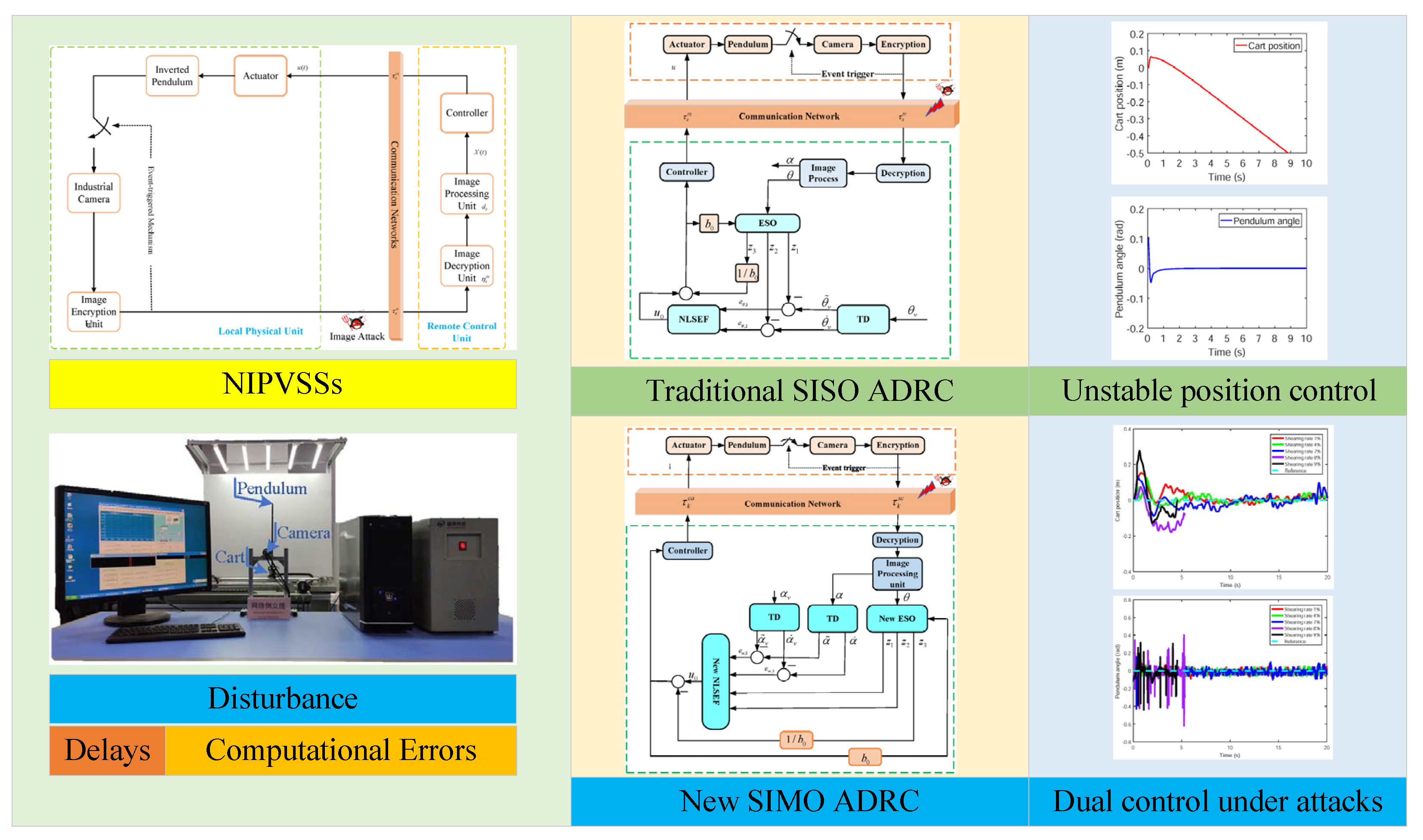
Figure 2.
Structure of NIPVSSs’ Fused Image Encryption and Decryption.
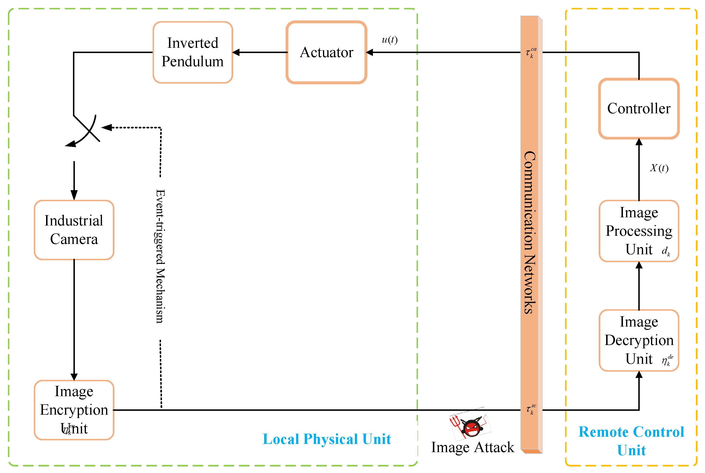
Figure 3.
NIPVSSs Model.

Figure 4.
Statistics of and .

Figure 5.
Typical second-order ADRC structure.
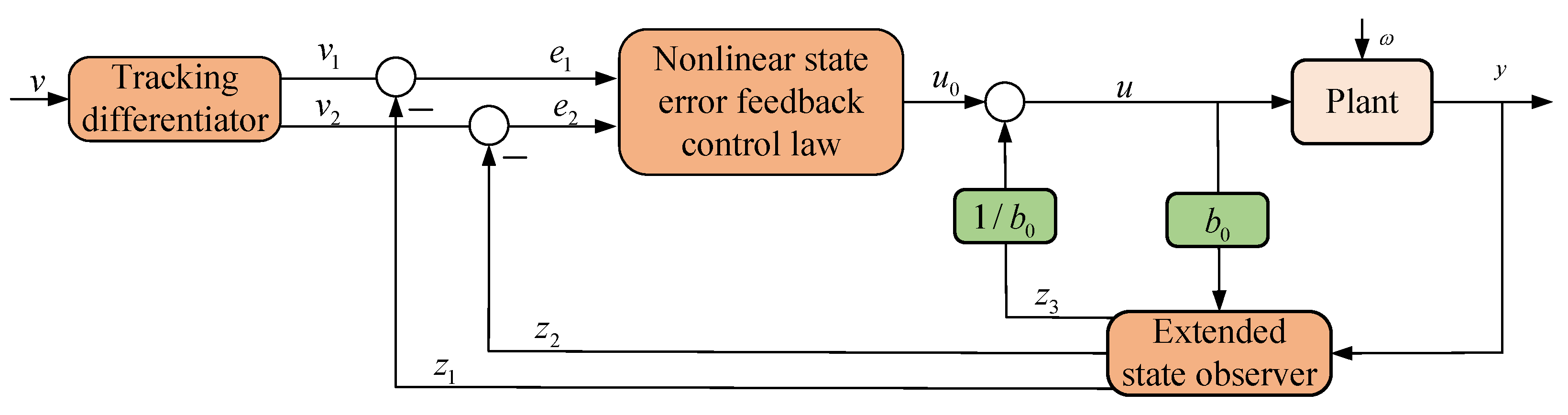
Figure 6.
Single-input-single-output ADRC with single target of pendulum angle.
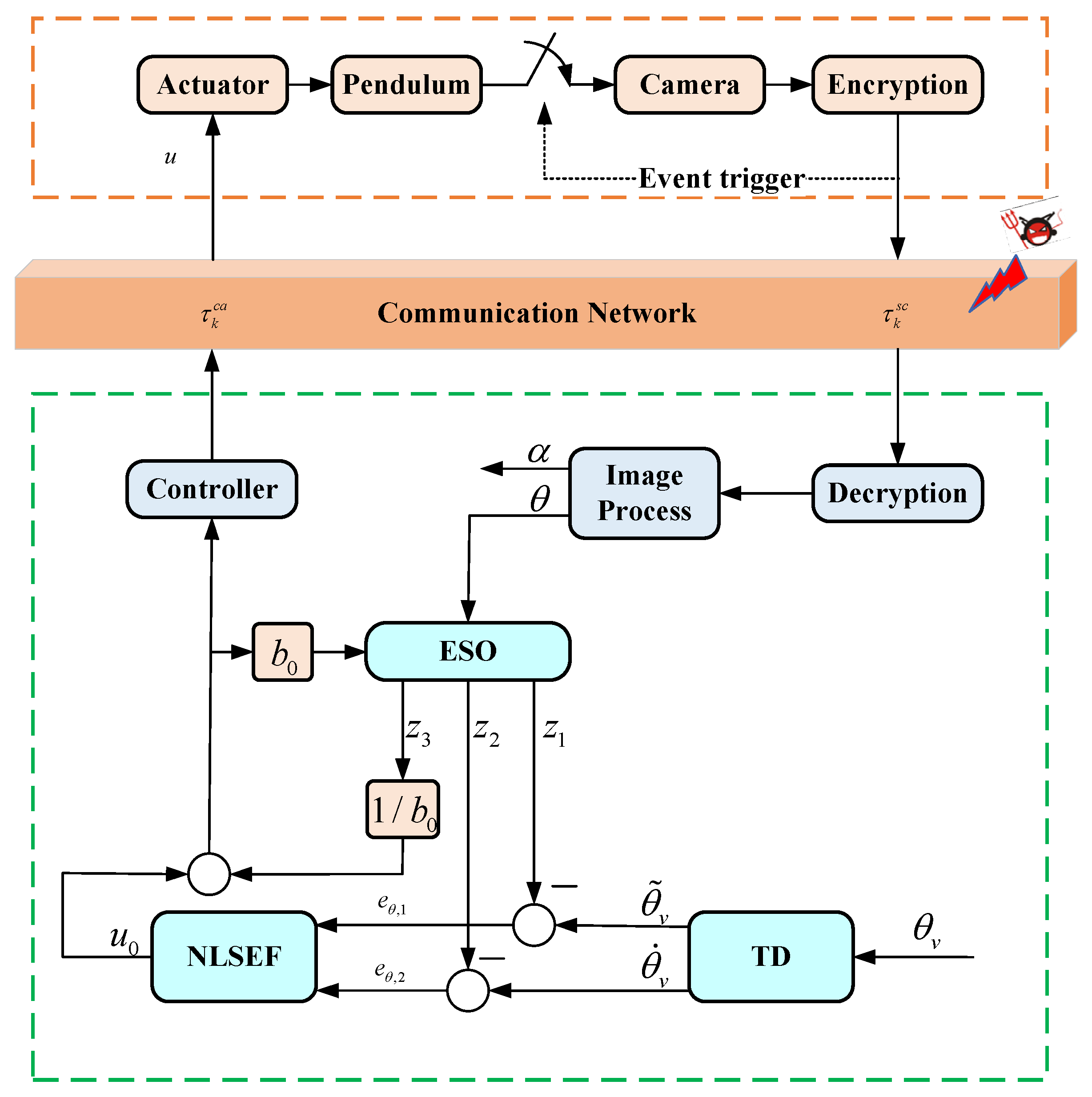
Figure 7.
Simulation results of traditional ADRC.
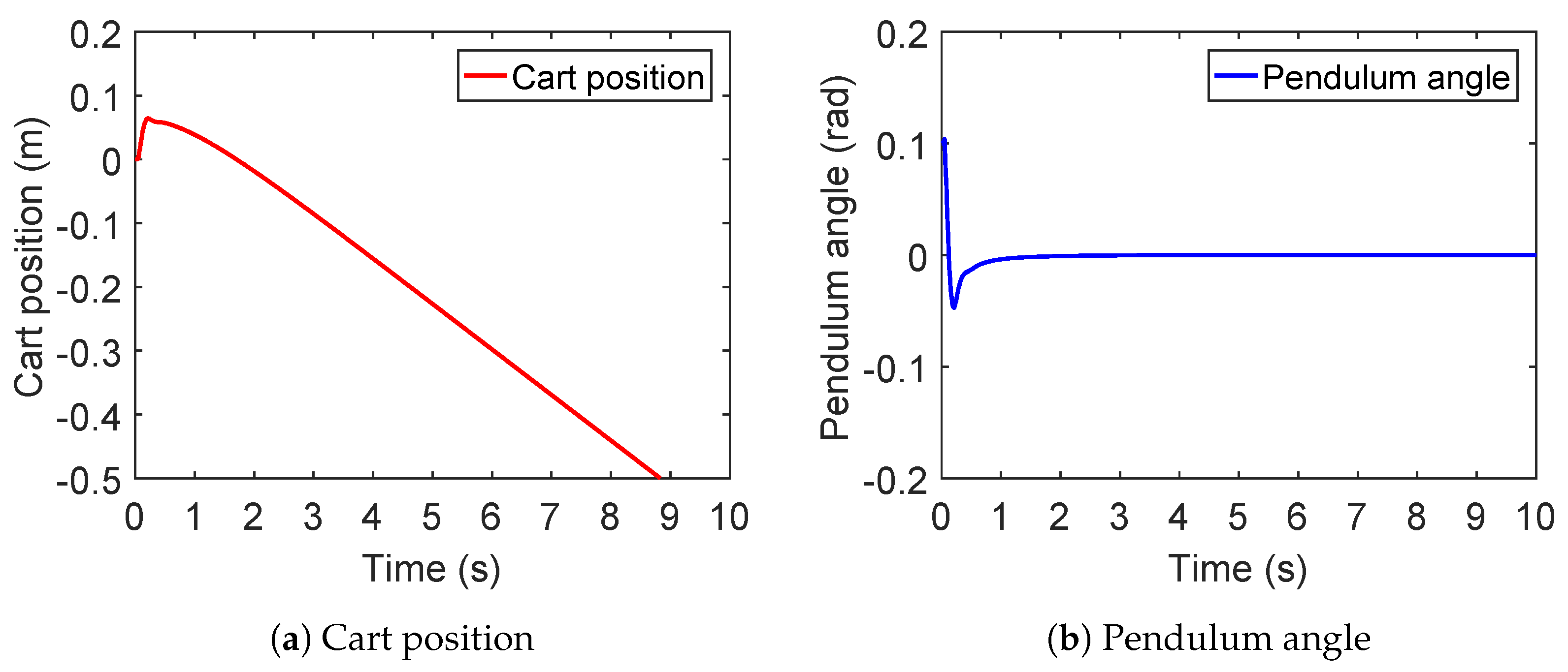
Figure 8.
Single-input-multi-output ADRC considering cart position and pendulum angle.

Figure 9.
Complete discrete-time improved ADRC algorithm.
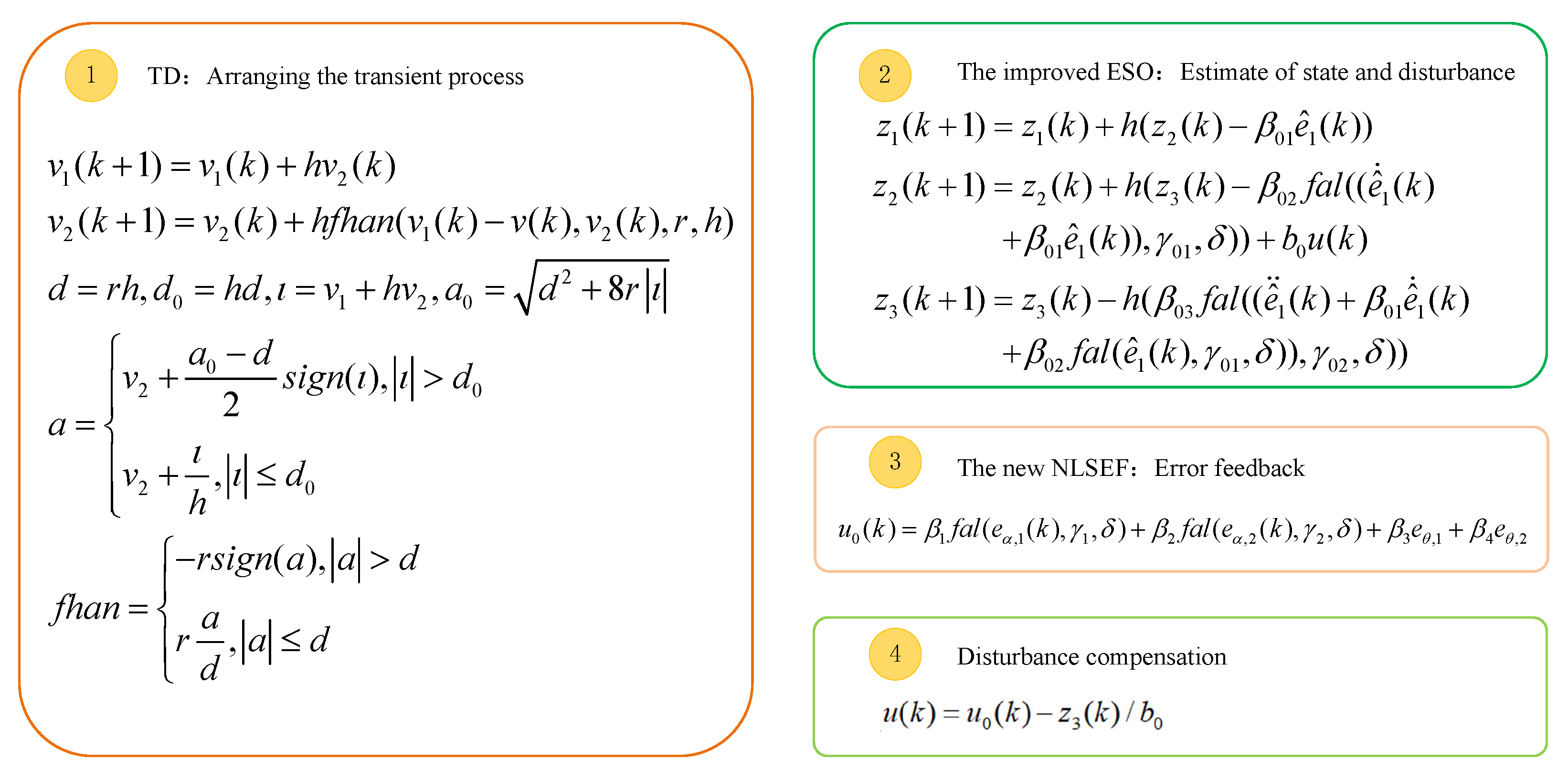
Figure 10.
Simulation results of single-input-multiple-output ADRC.
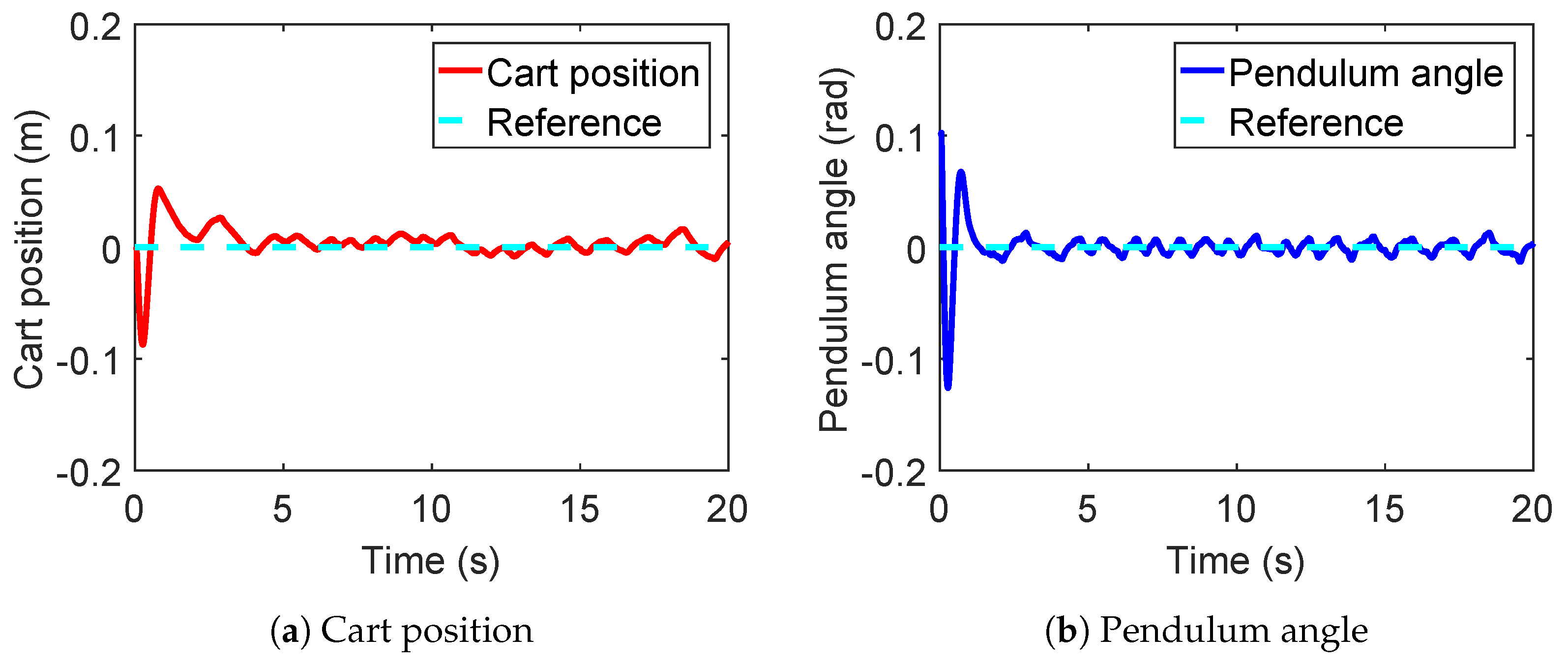
Figure 11.
Experimental results of single-input-multiple-output ADRC.
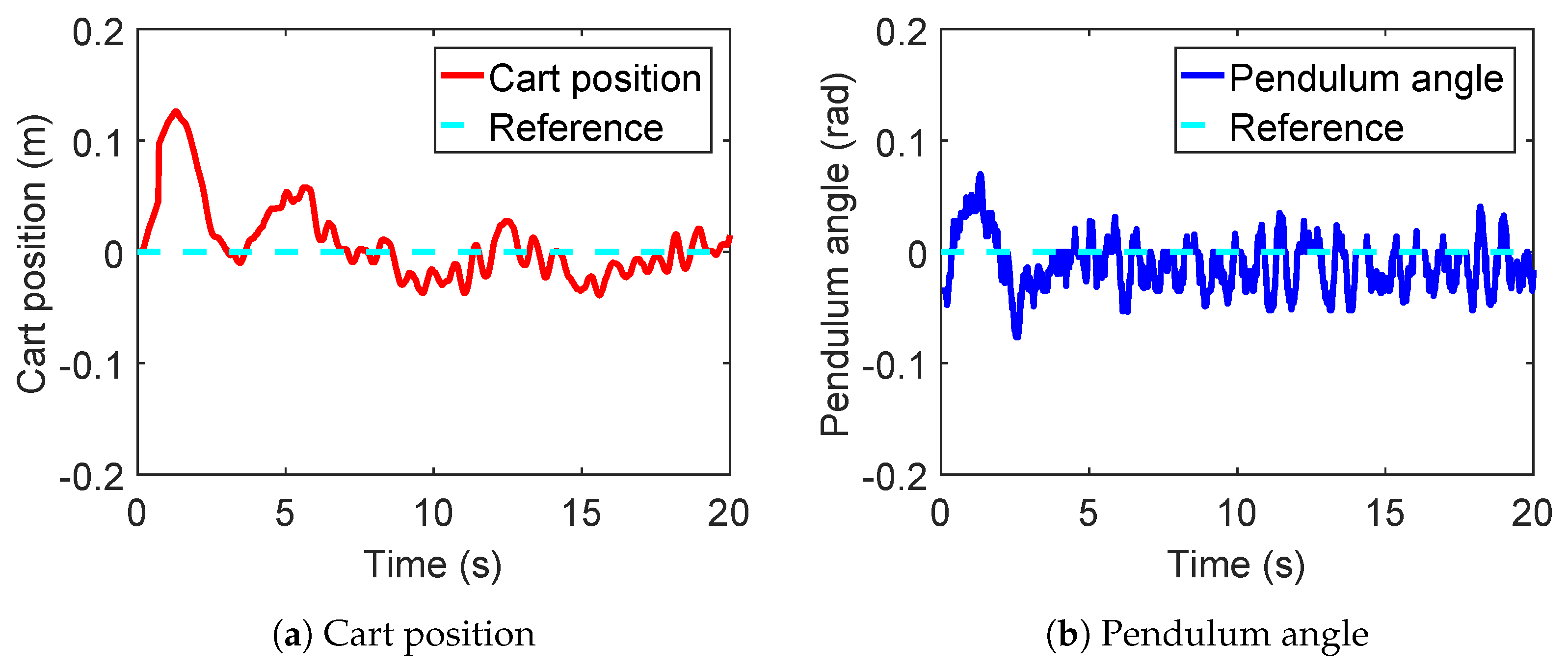
Figure 12.
Cart position (real-time control) under different intensities of salt and pepper attack.
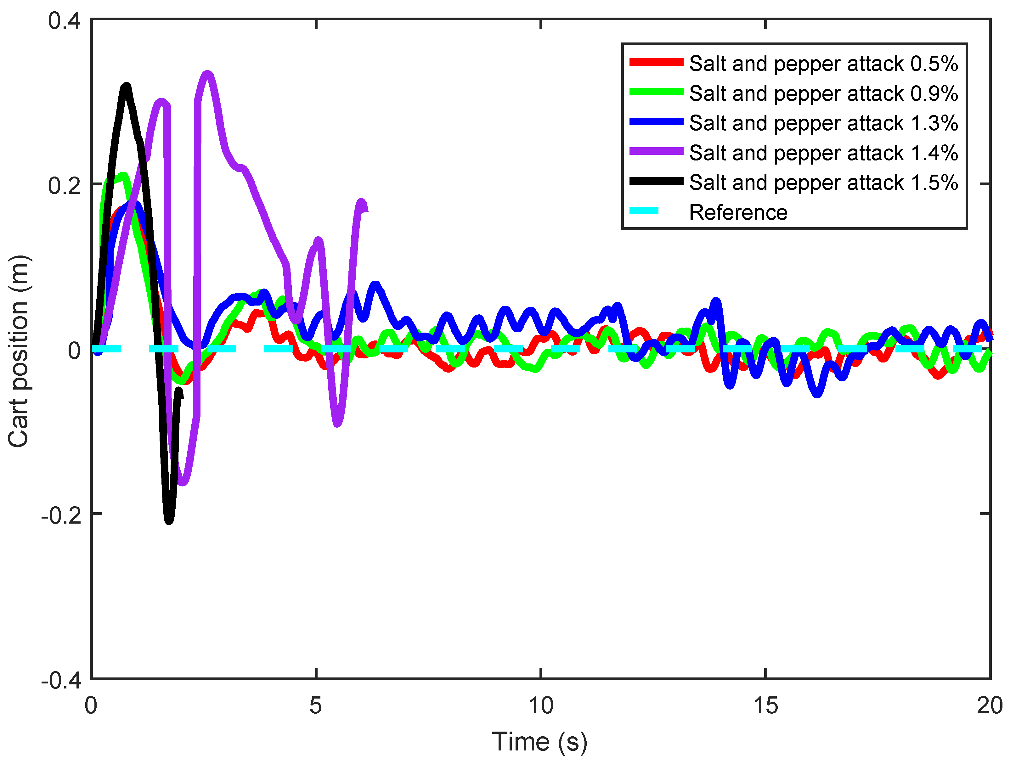
Figure 13.
Pendulum angle (real-time control) under different intensities of salt and pepper attack.
Figure 13.
Pendulum angle (real-time control) under different intensities of salt and pepper attack.
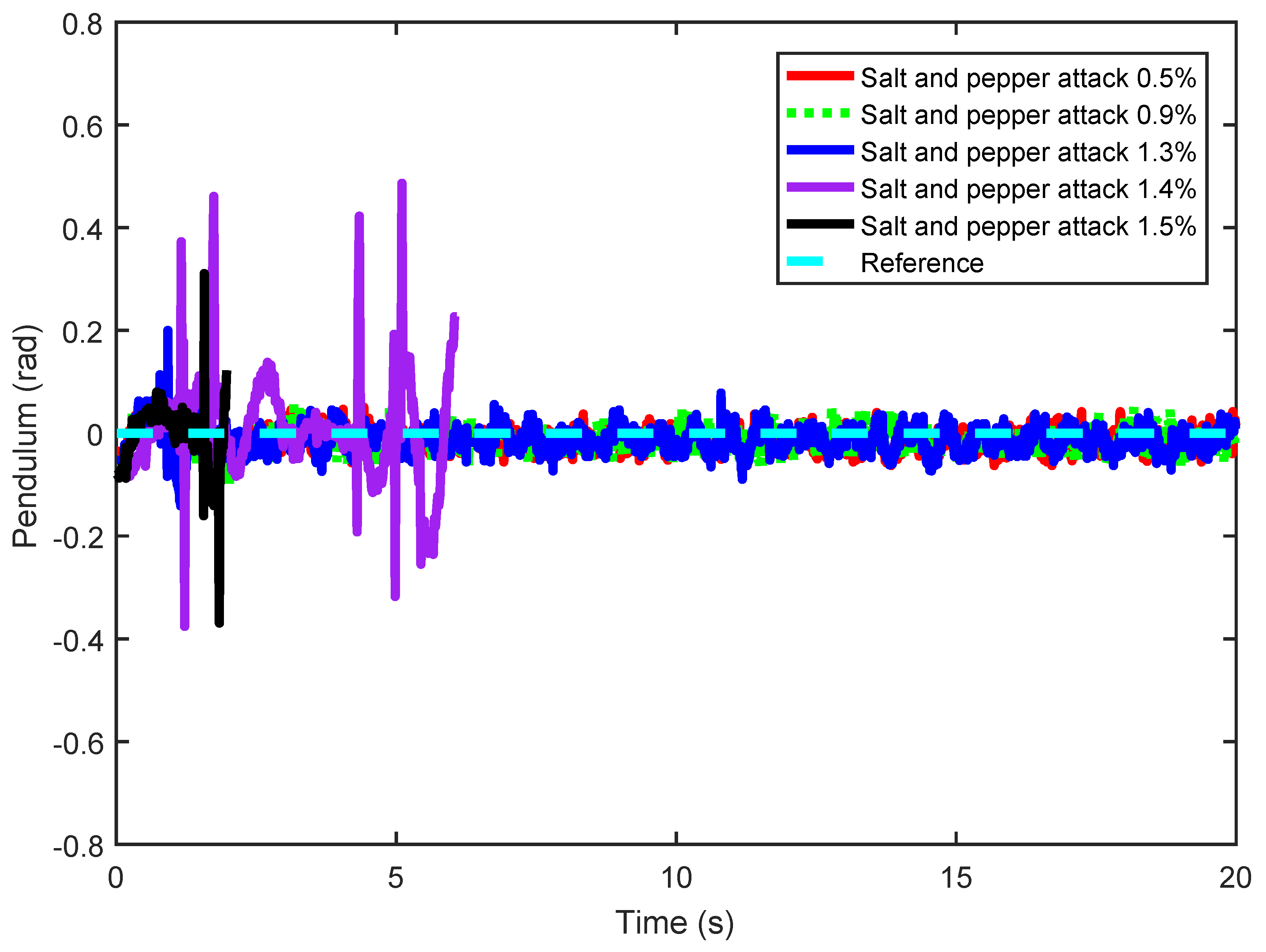
Figure 14.
Mean and standard deviation of cart position (real-time control) under different intensities of salt and pepper attack.
Figure 14.
Mean and standard deviation of cart position (real-time control) under different intensities of salt and pepper attack.
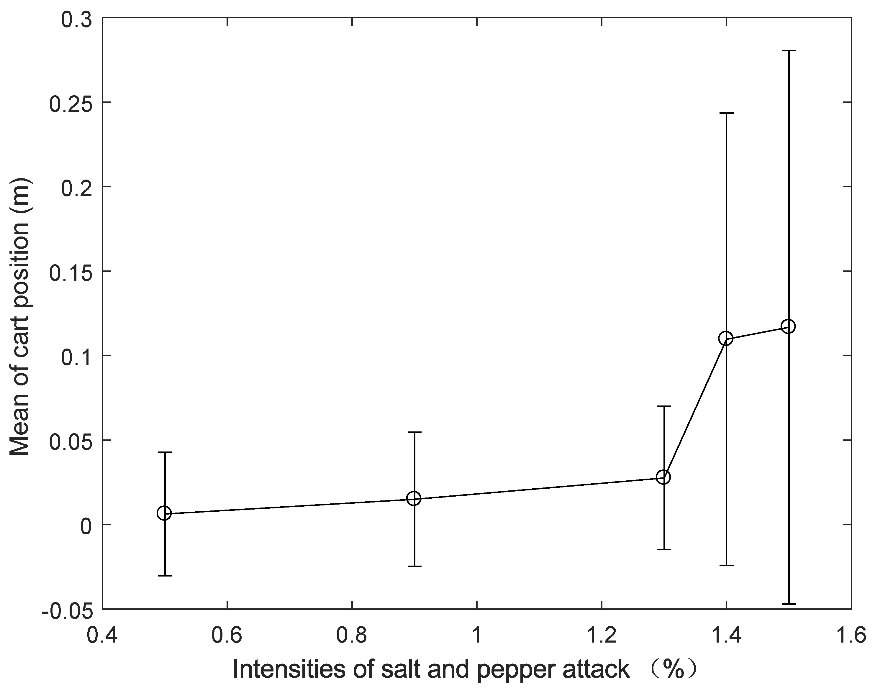
Figure 15.
Mean and standard deviation of pendulum angle (real-time control) under different intensities of salt and pepper attack.
Figure 15.
Mean and standard deviation of pendulum angle (real-time control) under different intensities of salt and pepper attack.
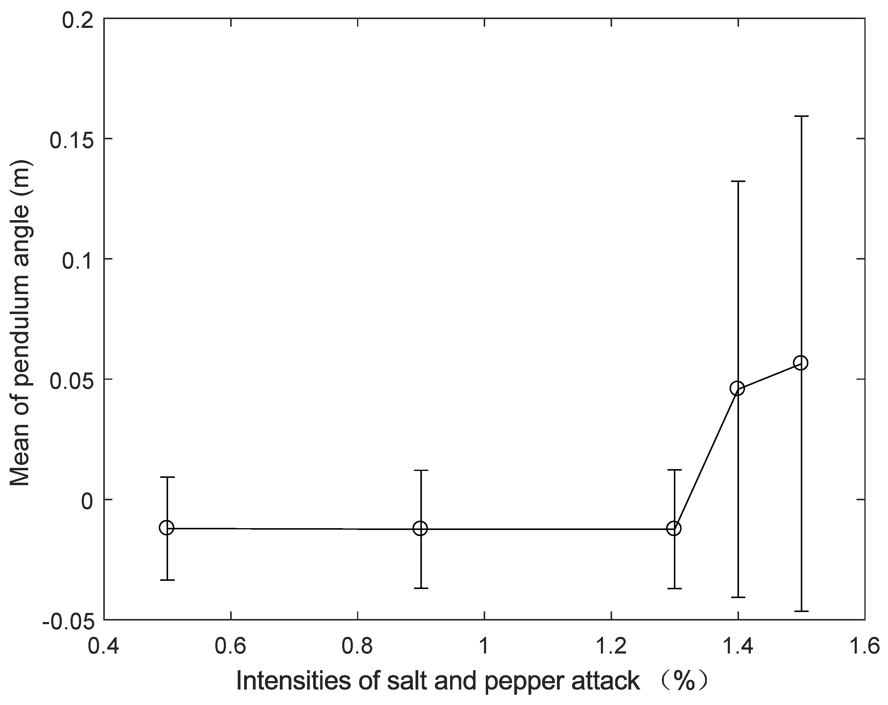
Figure 16.
Cart position (real-time control) under different intensities shearing rates.
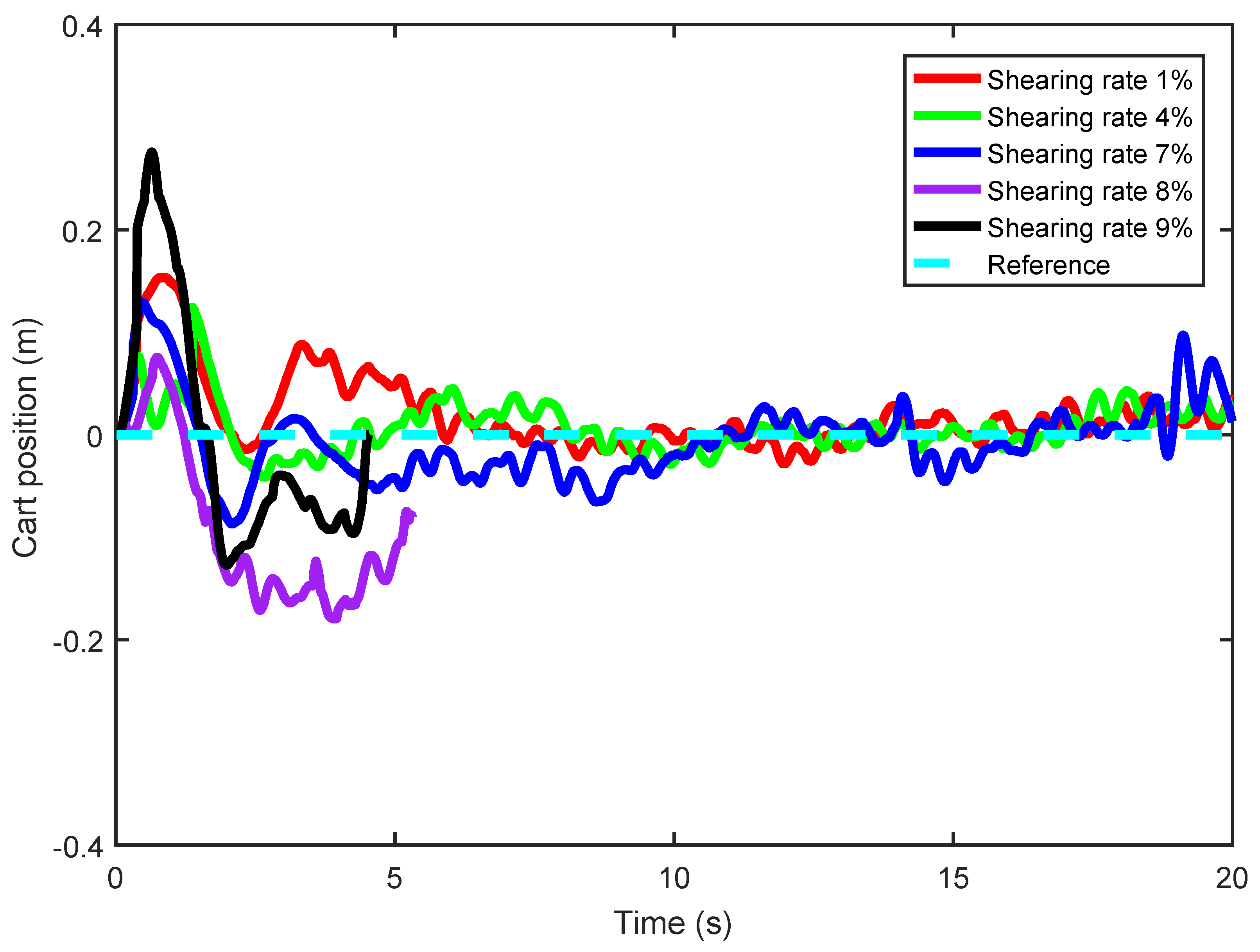
Figure 17.
Pendulum angle (real-time control) under different intensities shearing rates.

Figure 18.
Mean and standard deviation of cart position (real-time control) under different intensities shearing rates.
Figure 18.
Mean and standard deviation of cart position (real-time control) under different intensities shearing rates.
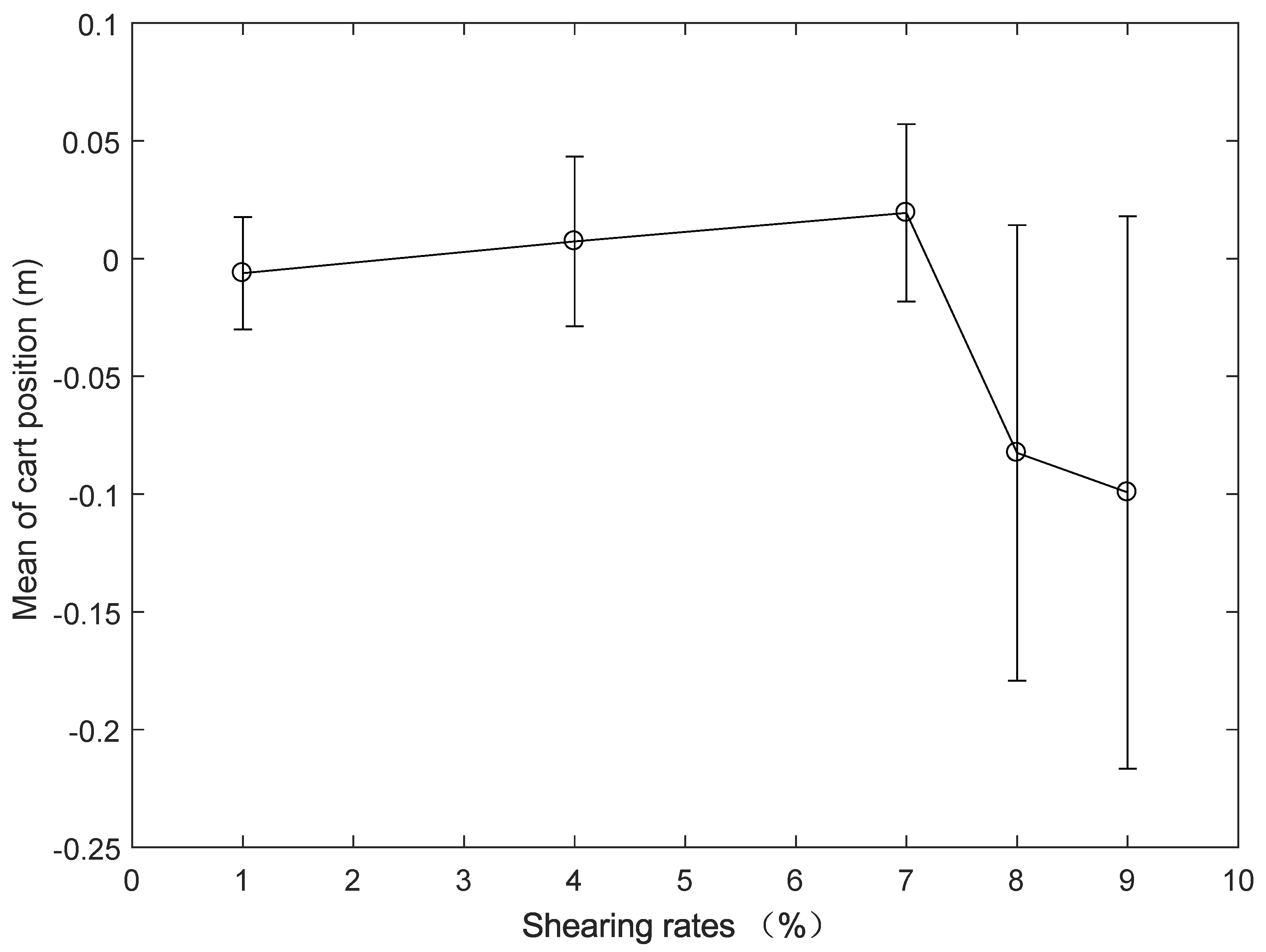
Figure 19.
Mean and standard deviation of pendulum angle (real-time control) under different intensities shearing rates.
Figure 19.
Mean and standard deviation of pendulum angle (real-time control) under different intensities shearing rates.

Figure 20.
Cart position (real-time control) under different distributions.
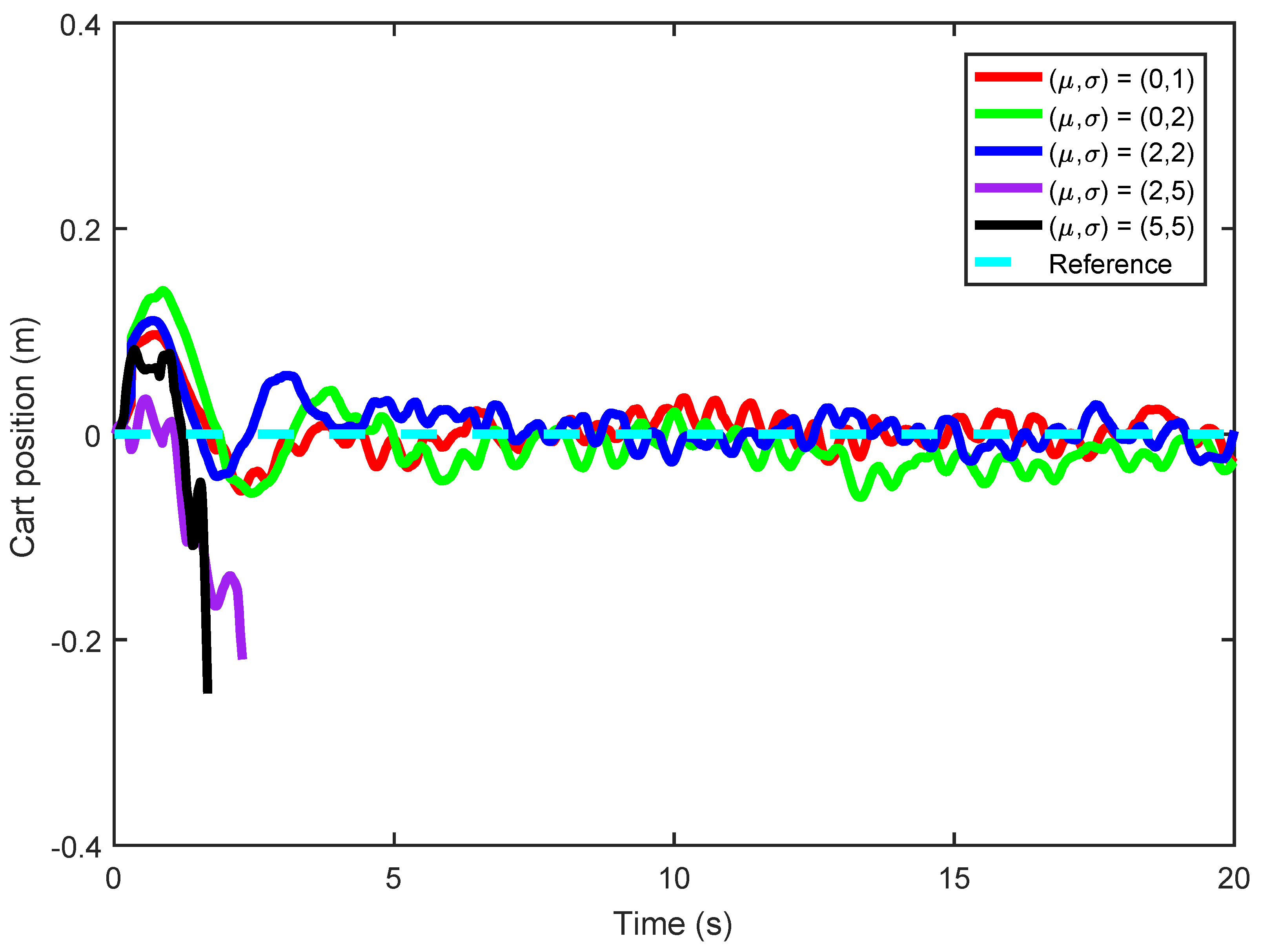
Figure 21.
Pendulum angle (real-time control) under different distributions.
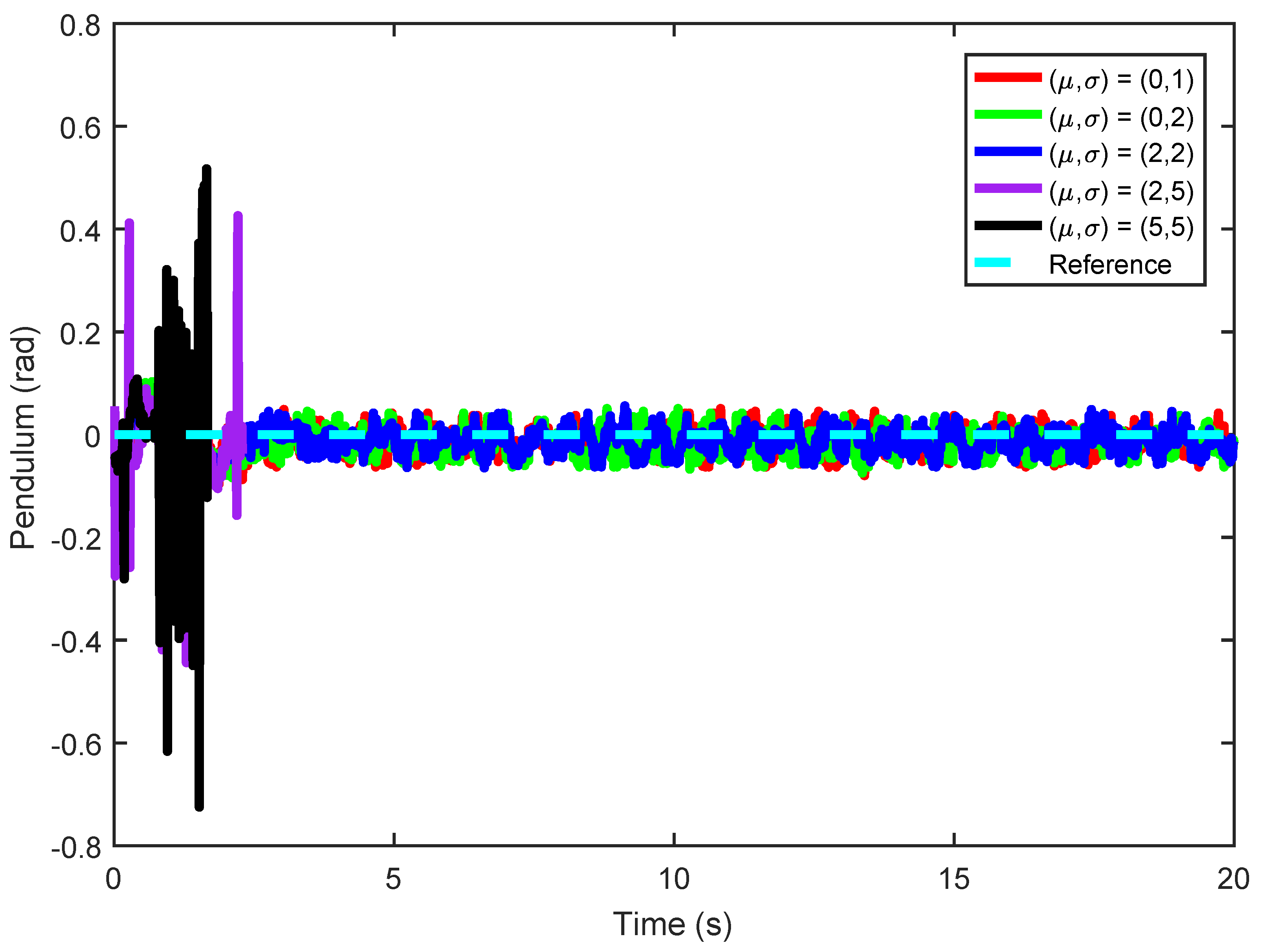
Figure 22.
Mean and standard deviation of cart position (real-time control) under different distributions.
Figure 22.
Mean and standard deviation of cart position (real-time control) under different distributions.
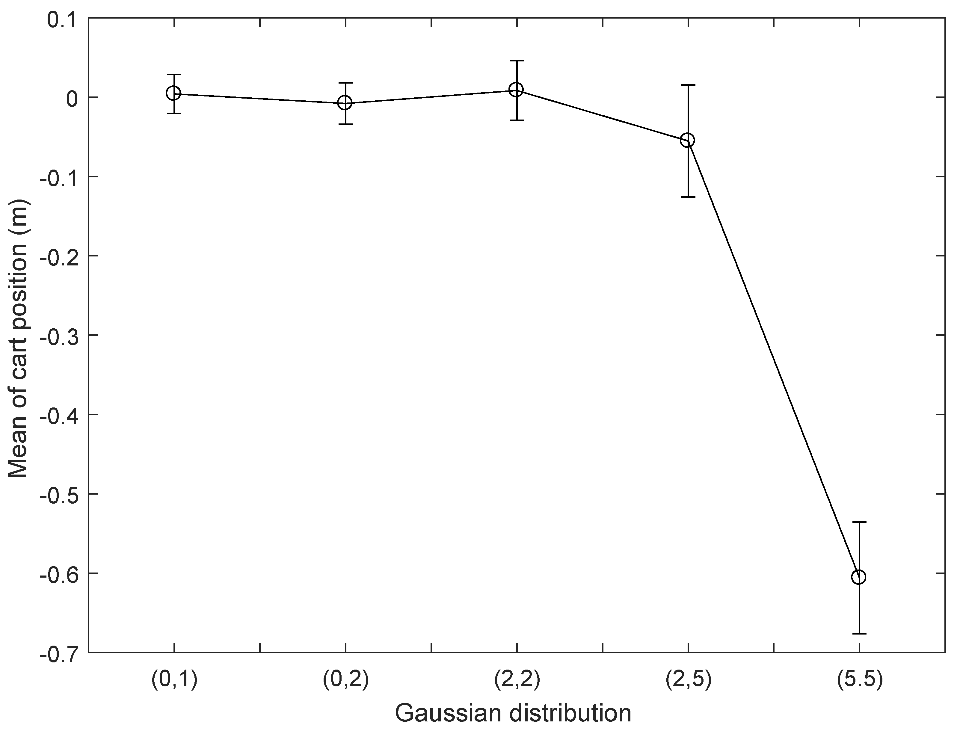
Figure 23.
Mean and standard deviation of pendulum angle (real-time control) under different distributions.
Figure 23.
Mean and standard deviation of pendulum angle (real-time control) under different distributions.

Figure 24.
Experimental results of NIPVSSs under salt and pepper attack at intensity of 0.5% and Gaussian attack simultaneously.
Figure 24.
Experimental results of NIPVSSs under salt and pepper attack at intensity of 0.5% and Gaussian attack simultaneously.
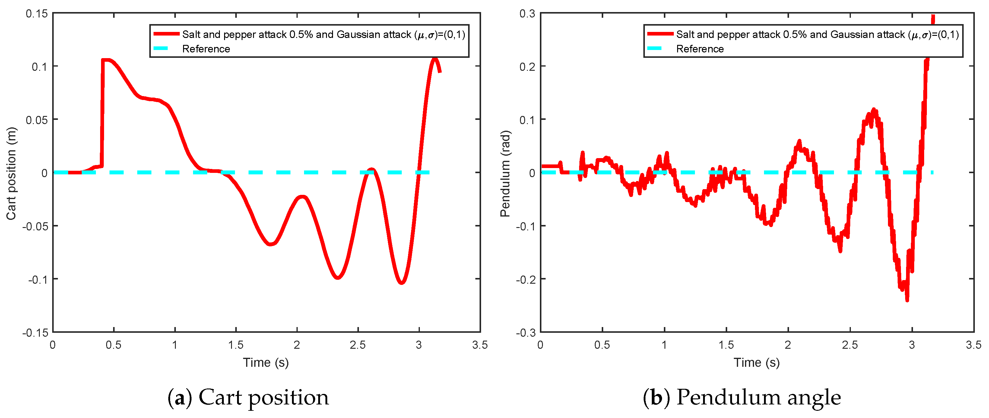
Figure 25.
Cart position and pendulum angle of the NIPVSSs with the controller in [13].
Figure 25.
Cart position and pendulum angle of the NIPVSSs with the controller in [13].
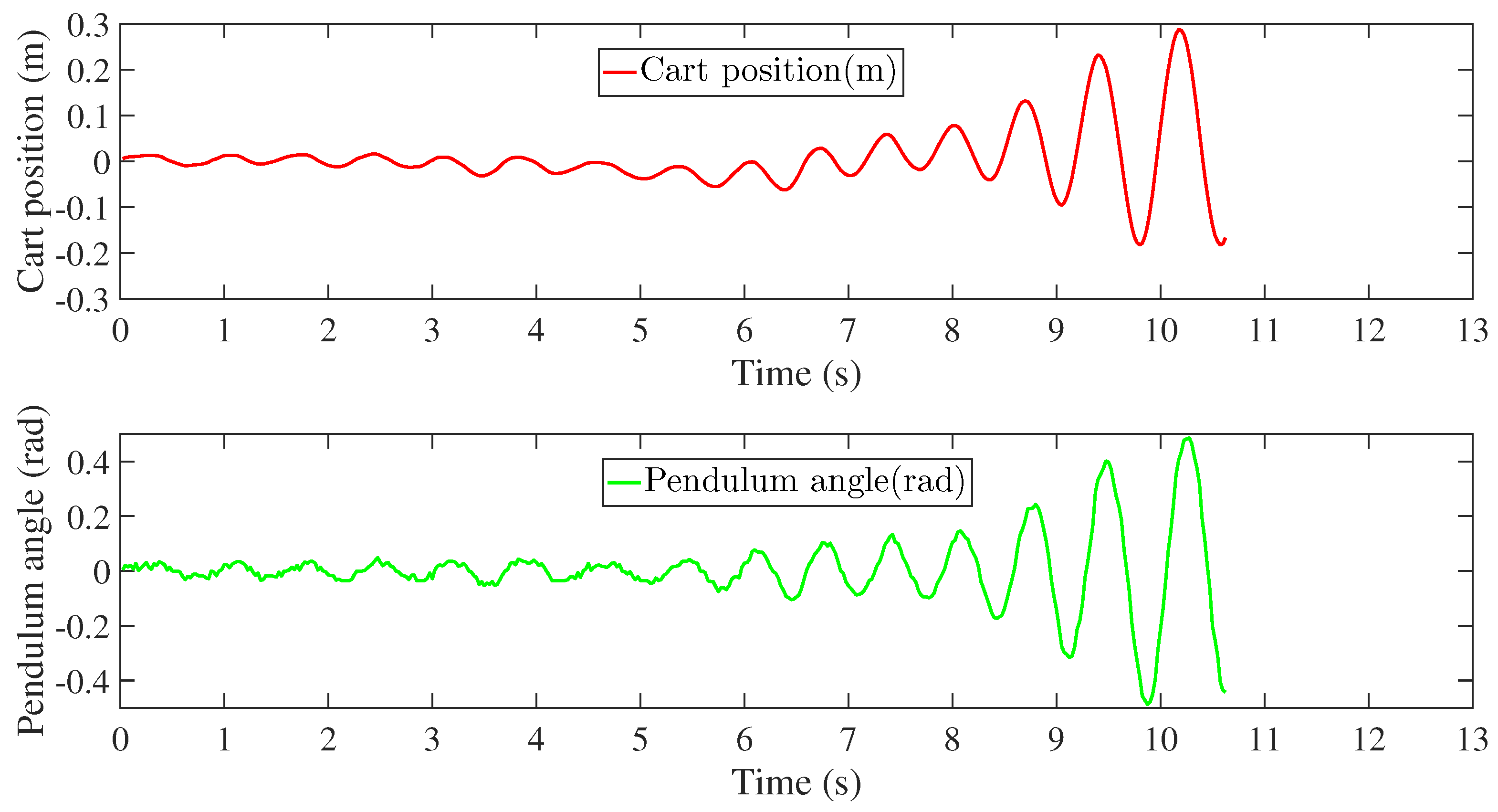
Figure 26.
Cart position and pendulum angle of the NIPVSSs with the sliding mode controller in [17].
Figure 26.
Cart position and pendulum angle of the NIPVSSs with the sliding mode controller in [17].


Table 1.
Comparison of steady-state errors between new ESO and traditional ESO.
| New ESO | |||
| Traditional ESO |
Table 2.
ADRC-based NIPVSSs parameters.
| Links | ESO Link | NLSEF Link |
|---|---|---|
| Parameters | , , , | , , , , |
Table 3.
Mean and standard deviation of cart position and pendulum angle under different intensities of salt and pepper attack.
Table 3.
Mean and standard deviation of cart position and pendulum angle under different intensities of salt and pepper attack.
| Intensities of Salt and Pepper Attack | 0.5% | 0.9% | 1.3% | 1.4% | 1.5% |
|---|---|---|---|---|---|
| MCP (m) | 0.0036 | 0.0150 | 0.0276 | 0.1097 | 0.1168 |
| SCP (m) | 0.0366 | 0.0397 | 0.0424 | 0.1338 | 0.1638 |
| MPA (rad) | −0.0121 | −0.0124 | −0.0124 | 0.0458 | 0.0564 |
| MPA (rad) | 0.0214 | 0.0245 | 0.0247 | 0.0865 | 0.1029 |
1 Mean of cart position 2 Standard deviation of cart position 3 Mean of pendulum angle 4 Standard deviation of pendulum angle.
Table 4.
Mean and standard deviation of cart position and pendulum angle under different shearing rate.
Table 4.
Mean and standard deviation of cart position and pendulum angle under different shearing rate.
| Shearing Rate | 1% | 4% | 7% | 8% | 9% |
|---|---|---|---|---|---|
| MCP (m) | −0.0062 | 0.0073 | 0.0194 | −0.0825 | −0.0993 |
| SCP (m) | 0.0239 | 0.0360 | 0.0377 | 0.0967 | 0.1173 |
| MPA (rad) | −0.0105 | −0.0127 | −0.0129 | 0.0424 | 0.0467 |
| MPA (rad) | 0.0257 | 0.0284 | 0.0366 | 0.0756 | 0.0790 |
1 Mean of cart position 2 Standard deviation of cart position 3 Mean of pendulum angle 4 Standard deviation of pendulum angle.
Table 5.
Mean and standard deviation of cart position and pendulum angle under Gaussian attack with distributions.
Table 5.
Mean and standard deviation of cart position and pendulum angle under Gaussian attack with distributions.
| (0,1) | (0,2) | (2,2) | (2,5) | (5,5) | |
|---|---|---|---|---|---|
| MCP (m) | 0.0041 | -0.0079 | 0.0085 | −0.0552 | −0.0606 |
| SCP (m) | 0.0246 | 0.0260 | 0.0374 | 0.0707 | 0.0705 |
| MPA (rad) | −0.0126 | −0.0128 | −0.0145 | 0.0106 | 0.0162 |
| MPA (rad) | 0.0252 | 0.0256 | 0.0280 | 0.0811 | 0.1750 |
1 Mean of cart position 2 Standard deviation of cart position 3 Mean of pendulum angle 4 Standard deviation of pendulum angle.
Publisher’s Note: MDPI stays neutral with regard to jurisdictional claims in published maps and institutional affiliations. |
© 2022 by the authors. Licensee MDPI, Basel, Switzerland. This article is an open access article distributed under the terms and conditions of the Creative Commons Attribution (CC BY) license (https://creativecommons.org/licenses/by/4.0/).
Share and Cite
MDPI and ACS Style
Wu, D.; Lu, Q. Secure Control of Networked Inverted Pendulum Visual Servo Systems Based on Active Disturbance Rejection Control. Actuators 2022, 11, 355. https://doi.org/10.3390/act11120355
AMA Style
Wu D, Lu Q. Secure Control of Networked Inverted Pendulum Visual Servo Systems Based on Active Disturbance Rejection Control. Actuators. 2022; 11(12):355. https://doi.org/10.3390/act11120355
Chicago/Turabian StyleWu, Dakui, and Qianjiang Lu. 2022. "Secure Control of Networked Inverted Pendulum Visual Servo Systems Based on Active Disturbance Rejection Control" Actuators 11, no. 12: 355. https://doi.org/10.3390/act11120355
Note that from the first issue of 2016, this journal uses article numbers instead of page numbers. See further details here.