
Output-Feedback Position Tracking Servo System with Feedback Gain Learning Mechanism via Order-Reduction Speed-Error-Stabilization Approach


1
Department of Electronic Engineering, Chosun University, Gwangju 61452, Korea
2
Department of Creative Convergence Engineering, Hanbat National University, Daejeon 34158, Korea
3
Department of ICT Convergence System Engineering, Chonnam National University, Gwangju 61186, Korea
*
Authors to whom correspondence should be addressed.
Actuators 2021, 10(12), 324; https://doi.org/10.3390/act10120324
Submission received: 29 October 2021
/
Revised: 1 December 2021
/
Accepted: 3 December 2021
/
Published: 5 December 2021
(This article belongs to the Special Issue Intelligent Control and Robotic System in Path Planning)
Abstract
:This paper presents a novel trajectory-tracking technique for servo systems treating only the position measurement as the output subject to practical concerns: system parameter and load uncertainties. There are two main contributions: (a) the use of observers without system parameter information for estimating the position reference derivative and speed and acceleration errors and (b) an order reduction exponential speed error stabilizer via active damping injection to enable the application of a feedback-gain-learning position-tracking action. A hardware configuration using a QUBE-servo2 and myRIO-1900 experimentally validates the closed-loop improvement under various scenarios.
1. Introduction
Servo systems play a pivotal role in determining the performance level of mechatronics system applications, including home appliances, personal mobility, factory machines, and so on. Increasing attention regarding the group motion control technology indicates the need for high technical specifications for these applications due to their safety and reliability specifications [1,2,3,4,5,6]. Recent synchronization techniques can be considered as a possible solution to this grouping control problem in industrial applications [7,8].
First, high-level closed-loop servo performance (speed and position control) must be secured to implement novel synchronization techniques with promising properties under various operating conditions. There are several types of motors, such as DC, brushless DC (BLDC), induction, and permanent magnet synchronous motors (PMSMs) available for the mechanical part of a servo system. Conventional (but simple) and advanced control techniques can be applied to implement closed-loop servo systems. The multi-loop proportional-integral (PI) controller, consisting of current (inner), speed (middle), and position (outer) loops, has normally been used to implement a closed-loop servo system whose feedback gain can be determined through trial-and-error and frequency-domain analysis tools (Bode and Nyquist plots) [9,10]. However, the tuning result is only feasible for a given operating point, and an additional gain scheduling technique must be used to widen the feasible operating region [11]. The feedback linearization-based multi-loop approach solves this problem by adding system-parameter-dependent compensation terms in the feed-forward loop, and their PI gains allow closed-loop dynamics governed by a first-order low-pass filter (LPF) using passive damping in an open-loop system [12]. The parameter dependence on the feed-forward terms and PI gains can be handled by adopting additional online parameter estimators as in [13,14,15]. Adaptive controllers have been recently suggested as a possible advanced solution to the speed tracking problem subject to parameter and load uncertainties, incorporating numerous parameter estimators [16,17,18]. Interestingly, an online self-tuner continuously updates the feedback gain according to an analytic rule to ensure closed-loop stability, but the optimality of the steady-state gain remains questionable [17]. A parameter-dependent observer that estimates both the state and disturbances was incorporated into a robust controller to enhance the disturbance attenuation performance of a closed-loop system [19]. In a separate study, a robust speed controller included a nonlinear disturbance observer (DOB) to estimate the desired feed-forward terms in order to secure improved closed-loop robustness and accuracy, which also alleviates the level of system-parameter dependence [20]. This type of DOB was adopted for a sliding-mode controller, including the discontinuous feedback loop, to reduce the chattering level during steady-state operation [21]. Alternatively, predictive controllers were used to pursue closed-loop optimality by predicting the state using system parameter and load information, incorporating a numerical optimization process online [22,23,24]. As another approach to the online self-tuning technique [17], an additional stabilizer for the self-tuner was included and used as a damping injection term in a proportional-type energy-shaping controller [25,26], which, however, limits the application area regarding speed regulation. There were several output-feedback controllers, including the extended state observer (ESO) involving the system parameter dependence (at least partially) and repetitive offline optimization process for an optimal observer gain [27,28,29].
This study attempts to solve the output-feedback position-tracking problem considering the challenges arising from previous results, corresponding to the exact servo system parameter information requirements (at least partially, for the controller and observers) and limiting the robustness associated with the integral actions and DOBs. The features (contributions) of the proposed tracking technique are summarized as follows:
- an extended state observer (for the position reference derivative and controlled errors involving speed and its acceleration) equipped with a specially structured tuning factor yielding the first-order exponential convergent estimation error behavior; and
- the combination of an active damping injection pole-zero cancellation PI controller and nonlinear DOB for the first-order exponential convergent speed error stabilizer without dependence on the exact servo system parameter values.
The resultant feedback system does not suffer from any magnitude or phase distortions between the reference and actual servo system position. The experimental setup using a QUBE-servo2 and myRIO-1900 indicates the feasibility of the proposed solution by experimentally showing the improvements in closed-loop performance.
2. Servo System Dynamics
This section introduces simple servo system dynamics by a DC power source (a DC motor and a brushless DC motor) to clarify the main idea behind this study. The input voltage (in V) applied to the stator initiates the stator current (in A) and rotor position (in rad) and speed (in rad/s), which forms a linear time-invariant system subject to the mismatched disturbance (the load torque in Nm) as follows:
with the output torque (in Nm), the back electromotive force (EMF) (in V) for some coefficients and ( for permanent magnet-type systems), and the system parameters of (rotor inertia in kgm), (rotor friction in Nm/rad/s), (stator inductance in mH), and (stator resistance in ).
The system parameters can experience dramatic variations depending on the operating conditions; thus, this study decomposes the original system parameters into their nominal values (provided by the manufacturer) and perturbation terms to address this practical challenging point (for instance, for the rotor inertia case). This yields another expression for the system representation (2) and (3) by combining them after applying an additional time derivative to the speed dynamics (2):
which has a known coefficient (its true version and variation ) and an unknown time-varying lumped disturbance . This representation resolves the two major problems associated with the plant-model mismatches caused by parameter and load variations.
3. Position-Tracking Control Law
3.1. Control Objective
Consider the first-order time-varying system for an error with a position reference trajectory , given by
with its base system defined by for some that satisfies
Note that the notation is used to abbreviate for convenience. This study chooses the time-varying system (5) as the desired closed-loop performance to achieve a superior convergence rate from its base system (6) by applying the boosting property , , as proved by Lemma 1 in Section 4. To attain this goal, the exponential convergence given by
is taken into account as the control objective of this study.
Remark 1.
The base system (6) can be written in low-pass filter (LPF) for slowly time-varying reference signals as
with its Laplace transform:
subject to the cut-off frequency in rad/s (or, equivalently, as in Hz). Therefore, the design parameter can be determined as the cut-off frequency of the LPF (8) for the mapping .
3.2. Position Control with Feedback-Gain-Learning Algorithm
The position dynamics (1) gives an equivalent form by introducing the additional design variable as
where , . This yields the open-loop position-error dynamics for the actual position error such that
where , which is treated as an unknown time-varying signal.
Remark 2.
In the case of a multi-servo system synchronization problem, the position reference can be given as a neighboring-stage servo system output, which can be solved by the proposed controller while ensuring the exponential convergence (7) so that . Considering a two multi-servo system example (where and denote the first and second system, respectively), it holds that , , , and .
3.2.1. Position Reference Derivative Observer
Consider the relationship and its decomposition with respect to the DC () and AC () components (e.g., and ). Then, it holds that
where and , , whose estimation can be accomplished by the proposed observer with its output error such that
with observer gains , , and state representing the estimate for . The proposed observer consisting of (11) and (12) forms the same structure as the conventional extended state observer (ESO), except for the gain structure design
for a given , which reduces the observer gain-tuning complexity, ensuring the first-order estimation error () convergence behavior. For details, see Section 4.
3.2.2. Position-Tracking Control
This subsection proposes a position-tracking control law for updating the design variable as
with the position-reference-derivative estimate obtained from the observer (11) and (12) and the feedback gain learning mechanism for such that
, driven by the nonlinear excitation term and error , according to the learning and restoration rates and . The nonlinearity in the feedback gain learning algorithm (14) makes it nontrivial for closed-loop stability analysis tasks. For more details, see Section 4.
3.3. Observer-Based Speed Error Stabilizer
3.3.1. Speed and Acceleration Error Observers
The proposed solution requires feedback involving the first and second derivatives (speed and acceleration) of the servo system position to stabilize the speed error dynamics and avoid the need for stator current measurements. It is difficult to extract the correct speed and acceleration trajectory by applying direct time differentiation to the position measurement owing to its high-frequency noise component. To overcome this system-parameter dependence problem, consider the relationship (acceleration), definition with , and decomposition with respect to the DC () and AC () components (e.g., and ). Then, it holds that
where and , , whose estimation can be obtained by the proposed observer with the output (so that and ) with error :
with observer gains , , and states and representing the estimates for and , respectively. The proposed observer consisting of (16)–(18) forms the same structure as the conventional ESO, except for the gain structure design:
for a given , which reduces the observer gain tuning complexity and ensures the first-order estimation error (, ) convergence behavior. For details, see Section 4.
3.3.2. Speed Error Stabilizer
The open-loop second-order speed dynamics (4) provide another expression regarding the error :
with the newly defined disturbance , whose servo system parameter information-free solution is proposed as
, with two tuning gains, and . Meanwhile, the observer-based nonlinear DOB estimates the disturbance by updating according to the following rule:
with gain . The proposed control law (20) exponentially stabilizes the speed error by reducing the second-order open-loop dynamics to first-order dynamics owing to the specially structured gains invoking the pole-zero cancellation. For details, see Section 4. Figure 1 shows the proposed output-feedback system structure.
4. Closed Loop Analysis
This section derives the beneficial closed-loop properties by analyzing the position control loop (Section 4.1), the speed error stabilization loop (Section 4.2), and the entire output-feedback system (Section 4.3).
4.1. Position Control Loop
This loop consists of three components: the feedback gain learning mechanism (14), the position reference derivative observers (11) and (12), and the control action (13). First, Lemma 1 presents the property of the gain learning mechanism (14) boosting the feedback gain such that , .
Lemma 1.
The feedback-gain learning mechanism (14) guarantees the attainment of the initial condition as the minimum value for , e.g.,
Proof.
Integrating the feedback gain learning mechanism (14) gives us
which indicates the existence of a lower bound of owing to the positive sign of . This completes the proof. □
Lemma 2 describes the output-error-convergence behavior driven by the position-reference-derivative observer (11) and (12), which plays a vital role in demonstrating the convergence property of its estimation error.
Lemma 2.
The position reference derivative observer (11) and (12) ensures the exponential convergence:
subject to the gain setting , where the desired trajectory represents the solution to the first-order convergent system:
Proof.
The output error gives second-order dynamics by combining (10), (11), and (12) such that
with its equivalent expression obtained from the Laplace transform:
where , which defines the performance error dynamics for as
These error dynamics yield the time derivative of the positive definite function with as
where Young’s inequality (, ) verifies the inequality above, which shows that (defining )
with . This completes the proof. □
Remark 3.
The result of Lemma 2 (exponential convergence (24)) makes it reasonable to assume that
which leads to the following chain of implications (using (11)):
Applying (26), this allows us to conclude that
which plays a vital role in demonstrating the beneficial position control loop property in Lemma 3.
Lemma 3.
The proposed position-tracking control loop shown in Figure 1 guarantees the -stability for the input-output mapping .
Proof.
The substitution of the proposed position-tracking control (13) into the open-loop dynamics (9) results in
which turns the positive definite function with (using (14) and (27)) into
with the application of Young’s inequality. The coefficient rearranges the upper bound of as
with , which shows the strict passivity for the mapping , indicating the stability [30]. This completes the proof. □
The inequality (29) supporting the result of Lemma 3 is the main purpose of this subsection, and it is used to prove the entire set of output-feedback system properties using Theorems 1 and 2 in Section 4.3.
4.2. Speed Error Stabilization Loop
This loop consists of three components: the speed and acceleration error observer (16)–(18), the DOB (21) and (22), and the control action (20). First, Lemma 2 provides the output error convergence behavior driven by the speed and acceleration error observer (16)–(18), which plays a vital role in showing the estimation error’s convergence property.
Lemma 4.
The speed and acceleration error observer (16)–(18) ensures the exponential convergence
subject to the gain setting , where the desired trajectory represents the solution to the first-order convergent system:
Proof.
The output error inherits third-order dynamics through the combination of (15)–(18) such that
with the equivalent expression obtained from the Laplace transform:
where and , which defines the performance error dynamics for as
These error dynamics yield the time derivative of the positive definite function with and as
with the application of the Young’s inequality. The coefficients and rearrange the upper bound of as
with , which completes the proof. □
Remark 4.
The result of Lemma 2 makes it reasonable to assume that
which leads to the following chain of implications (using (11)):
From (31), this indicates that , , which, together with (17) and following the same reasoning process above, yields , . Thus, the corresponding vector form for is obtained as
which plays a vital role in showing the beneficial closed-loop properties described by Theorems 1 and 2 in Section 4.3.
Lemma 5 presents the motion of the disturbance estimate governed by the observer-based nonlinear DOB (21) and (22).
Lemma 5.
The observer-based nonlinear DOB (21) and (22) drives the disturbance estimate to satisfy
for some constant vector .
Proof.
The time derivative of the output (22) is obtained along the dynamics (21) as
where the result of Remark 4 verifies the third equality above, which completes the proof. □
The definition of the disturbance estimation error , together with (33), gives
with and , , which is used in the proofs for Theorems 1 and 2 in Section 4.3. Lemma 6 provides the closed-loop speed error behavior governed by the control action (20) causing the order reduction because of the pole-zero cancellation nature.
Lemma 6.
The proposed speed error stabilization loop shown in Figure 1 guarantees the perturbed first-order speed error dynamics
with the filtered signal such that
for some constant , and constant vector .
Proof.
The substitution of the proposed speed error stabilizer (20) into the open-loop dynamics (19) results in
where (such that ) and , whose equivalent form is obtained by taking the Laplace transform of both sides:
. This causes the order reduction through the factorization such that
with , which completes the proof by taking the inverse Laplace transform. □
The closed-loop speed error dynamics (35) and (36) as the main results of this subsection help to prove the useful closed-loop properties described by Theorems 1 and 2 in Section 4.3.
4.3. Entire System Properties
This subsection provides the main analysis results using the subsystem properties given by Lemmas 1–6. Theorem 1 proves the boundedness property of the position error controlled by the proposed output-feedback system shown in Figure 1.
Theorem 1.
The proposed output-feedback system shown in Figure 1 guarantees the boundedness property
for some constant , .
Proof.
Considering (35) and (36), it follows from that
where and . The stability of ensures the existence of the unique solution to the matrix equation , which defines the positive definite function as
whose time derivative is obtained using (29), (32), (34), and (38):
The coefficients , , and rearrange the upper bound of as
with . This completes the proof by using the comparison principle in [30]. □
Theorem 1 roughly derives the exponential position convergence
with a large DOB gain such that by showing that , , from inequality (39), which is assumed when proving the main result in Theorem 2.
Theorem 2.
Proof.
Defining the performance error as means that
which turns the composite-type positive definite function
into (using feedback gain boosting property shown in Lemma 1)
with the application of Young’s inequality. The coefficient rearranges the upper bound of as
where , which completes the proof. □
5. Experimental Results
This section provides experimental comparison data as actual evidence that demonstrates the effectiveness of the proposed technique. Data were obtained from the experimental platform in Figure 2 comprising the QUBE-servo2 (servo system), myRIO-1900 (processor), and LabVIEW software. The nominal servo system parameters were set as , , , , and , based on manufacturer values , , , , , and (see the datasheet provided by Quanser). The MathScript in LabVIEW software implemented the control and estimation algorithms under control and sampling periods of ms.
The tuning result of the proposed controller is given by: (position reference derivative observer) , (position-tracking control) Hz ( rad/s), , , (speed and acceleration error observers) , (speed error stabilizer) , , and (DOB) .
An integral back-stepping controller (IBSC) including the active-damping injection term was used for the comparison study, which is given by (position loop) , (speed loop) , , (current loop) , and , with its tuning results: (active damping) , , (speed and current cut-off frequencies) rad/s, rad/s.
The positioning performances of these two controllers were evaluated under the tracking and regulation tasks for two different loads—disc and pendulum loads—to clarify the closed-loop robustness improvement against load variations.
5.1. Reference Trajectory Tracking Performance
This subsection highlights the performance improvement by investigating the position tracking behavior for two different cases: a piece-wise constant reference (in stair form) and sinusoidal references.
5.1.1. Case I: Stair Reference
This experiment sets the position reference to zero initially and increases and decreases it to 20 and sequentially. Figure 3 indicates the position tracking behaviors using the proposed and IBSC techniques and shows that the proposed controller shortens the transient periods without any over-/undershoots with the cooperation of the feedback-gain learning mechanism that ensures the boosting property proven in Lemma 1.
The left panel of Figure 4 presents the actual position feedback gain responses from the feedback-gain learning mechanism (14). The right panel of Figure 4 shows the observer-based nonlinear DOB responses. Figure 5 indicates the rapid state estimation error removal performance from the speed and acceleration error observers, leading to the closed-loop performance improvement shown in Figure 3.
5.1.2. Case II: Sinusoidal Reference
This experiment considered three different sinusoidal position references increasing in frequency 1, 5, and 15 Hz under the pendulum load condition. As indicated in Figure 6, a significant performance improvement was observed owing to the perfect trajectory tracking nature of the proposed technique without any distortion between the reference and the actual servo system position. The exponential convergence property proven in Theorem 2 provides this meaningful advantage in cooperation with the novel subsystems shown in Figure 1.
5.2. Constant Reference Regulation Performance
This experiment fixed the position reference to zero while a load torque ( Nm, requiring a stator current A, as shown in Figure 8) was suddenly applied to the closed-loop system. Figure 7 presents a considerable regulation performance improvement using the proposed controller, eliminating the transient periods despite the abrupt change in load condition. The corresponding dynamic current responses are shown in Figure 8, which shows that there were no significant differences from the current responses driven by the proposed and IBSC technique, but in improvement in the position regulation performance was observed, as shown in Figure 7, due to the novel subsystems for the position loop.
6. Conclusions
This study proposes an advanced solution to the position-tracking problem for servo systems, incorporating intelligence and improved robustness in the feedback loop. The systematic controller design process not only results in beneficial closed-loop properties by analyzing the closed-loop dynamics, but also provides a significant tracking performance improvement for time-varying reference trajectories without any phase delay or magnitude distortions based on the experimental study results. This result will be extended to multi-servo system synchronization applications, considering the interactions between local agents as disturbances, in a future study.
Author Contributions
Conceptualization and methodology, S.-K.K.; software, validation, formal analysis, investigation, writing—original draft preparation, and writing—review and editing, S.H.Y.; resources, supervision, project administration, and funding acquisition, H.D.C. All authors have read and agreed to the published version of the manuscript.
Funding
This research was supported by the research fund of Hanbat National University in 2021.
Institutional Review Board Statement
Not applicable.
Informed Consent Statement
Not applicable.
Data Availability Statement
Data sharing not applicable.
Conflicts of Interest
The authors declare no conflict of interest.
References
- Wang, P.; Zhu, L.; Zhang, C.; Wang, C.; Xiao, K. Prescribed Performance Control with Sliding-Mode Dynamic Surface for a Glue Pump Motor Based on Extended State Observers. Actuators 2021, 10, 282. [Google Scholar] [CrossRef]
- Suti, A.; Di Rito, G.; Galatolo, R. Fault-Tolerant Control of a Three-Phase Permanent Magnet Synchronous Motor for Lightweight UAV Propellers via Central Point Drive. Actuators 2021, 10, 253. [Google Scholar] [CrossRef]
- Božek, P.; Nikitin, Y. The Development of an Optimally-Tuned PID Control for the Actuator of a Transport Robot. Actuators 2021, 10, 195. [Google Scholar] [CrossRef]
- Ismail, M.; Wiedemann, S.; Bosch, C.; Stuckmann, C. Design and Evaluation of Fault-Tolerant Electro-Mechanical Actuators for Flight Controls of Unmanned Aerial Vehicles. Actuators 2021, 10, 175. [Google Scholar] [CrossRef]
- Kim, S.K.; Ahn, C.K. Active-damping Speed Tracking Technique for Permanent Magnet Synchronous Motors with Transient Performance Boosting Mechanism. IEEE Trans. Ind. Inf. 2021, 1, 1–9. [Google Scholar] [CrossRef]
- Park, J.K.; Lee, J.H.; Kim, S.K.; Ahn, C.K. Output-Feedback Speed-Tracking Control Without Current Feedback for BLDCMs Based on Active-Damping and Invariant Surface Approach. IEEE Trans. Circuits Syst. II Express Briefs 2021, 68, 2528–2532. [Google Scholar] [CrossRef]
- Lin, C.H.; Ho, C.W.; Hu, G.H.; Sreeramaneni, B.; Yan, J.J. Secure Data Transmission Based on Adaptive Chattering-Free Sliding Mode Synchronization of Unified Chaotic Systems. Mathematics 2021, 9, 2658. [Google Scholar] [CrossRef]
- Li, M.; Zhang, R.; Yang, S. Adaptive Synchronization of Fractional-Order Complex-Valued Chaotic Neural Networks with Time-Delay and Unknown Parameters. Physics 2021, 3, 924–939. [Google Scholar]
- Andeescu, G.D.; Pitic, C.; Blaabjerg, F.; Boldea, I. Combined flux observer with signal injection enhancement for wide speed range sensorless direct torque control of IPMSM drives. IEEE Trans. Energy Convers. 2008, 23, 393–402. [Google Scholar] [CrossRef]
- Tang, L.; Zhong, L.; Rahman, M.; Hu., Y. A novel direct torque control for interior permanent-magnet synchronous machine drive with low ripple in torque and flux—A speed-senseroless approach. IEEE Trans. Ind. Appl. 2003, 39, 1748–1756. [Google Scholar] [CrossRef]
- Olalla, C.; Leyva, R.; Queinnec, I.; Maksimovic, D. Robust Gain-Scheduled Control of Switched-Mode DC-DC Converters. IEEE Trans. Power Electron. 2012, 27, 3006–3019. [Google Scholar] [CrossRef]
- Sul, S.K. Control of Electric Machine Drive Systems; Wiley: Hoboken, NJ, USA, 2011; Volume 88. [Google Scholar]
- Sengupta, I.; Gupta, S.; Deb, D.; Ozana, S. Dynamic Stability of an Electric Monowheel System Using LQG-Based Adaptive Control. Appl. Sci. 2021, 11, 9766. [Google Scholar] [CrossRef]
- Wang, J.; Chen, Z. Variational Bayesian Iteration-Based Invariant Kalman Filter for Attitude Estimation on Matrix Lie Groups. Aerospace 2021, 8, 246. [Google Scholar] [CrossRef]
- Huang, H.; Tang, J.; Zhang, B. Positioning Parameter Determination Based on Statistical Regression Applied to Autonomous Underwater Vehicle. Appl. Sci. 2021, 11, 7777. [Google Scholar] [CrossRef]
- Kim, S.K.; Lee, J.S.; Lee, K.B. Self-Tuning Adaptive Speed Controller for Permanent Magnet Synchronous Motor. IEEE Trans. Power Electron. 2017, 32, 1493–1506. [Google Scholar] [CrossRef]
- Kim, S.K. Robust adaptive speed regulator with self-tuning law for surfaced-mounted permanent magnet synchronous motor. Control Eng. Pract. 2017, 61, 55–71. [Google Scholar] [CrossRef]
- El-Sousy, F.F.M.; Abuhasel, K.A. Nonlinear Robust Optimal Control via Adaptive Dynamic Programming of Permanent-Magnet Linear Synchronous Motor Drive for Uncertain Two-Axis Motion Control System. IEEE Trans. Ind. Appl. 2020, 56, 1940–1952. [Google Scholar] [CrossRef]
- Errouissi, R.; Ouhrouche, M.; Chen, W.H.; Trzynadlowski, A.M. Robust Cascaded Nonlinear Predictive Control of a Permanent Magnet Synchronous Motor With Antiwindup Compensator. IEEE Trans. Ind. Electron. 2012, 59, 3078–3088. [Google Scholar] [CrossRef]
- Son, Y.I.; Kim, I.H.; Choi, D.S.; Shim, H. Robust Cascade Control of Electric Motor Drives Using Dual Reduced-Order PI Observer. IEEE Trans. Ind. Electron. 2015, 62, 3672–3682. [Google Scholar] [CrossRef]
- Corradini, M.L.; Ippoliti, G.; Longhi, S.; Orlando, G. A Quasi-Sliding Mode Approach for Robust Control and Speed Estimation of PM Synchronous Motors. IEEE Trans. Ind. Electron. 2012, 59, 1096–1104. [Google Scholar] [CrossRef]
- Geyer, T.; Papafotieu, G.; Morari, M. Model predictive direct torque control-part I: Concept, algorithm and analysis. IEEE Trans. Ind. Electron. 2009, 56, 1894–1905. [Google Scholar] [CrossRef]
- Ahmed, A.A.; Koh, B.K.; Lee, Y.I. A Comparison of Finite Control Set and Continuous Control Set Model Predictive Control Schemes for Speed Control of Induction Motors. IEEE Trans. Ind. Inf. 2018, 14, 1334–1346. [Google Scholar] [CrossRef]
- Tao, T.; Zhao, W.; Du, Y.; Cheng, Y.; Zhu, J. Simplified Fault-Tolerant Model Predictive Control for a Five-Phase Permanent-Magnet Motor with Reduced Computation Burden. IEEE Trans. Power Electron. 2020, 35, 3850–3858. [Google Scholar] [CrossRef]
- Kim, S.K.; Kim, Y.; Ahn, C.K. Energy-Shaping Speed Controller with Time-Varying Damping Injection for Permanent-Magnet Synchronous Motors. IEEE Trans. Circuits Syst. II Express Briefs 2021, 68, 381–385. [Google Scholar] [CrossRef]
- Kim, S.K.; Ahn, C.K. Position Regulator with Variable Cut-Off Frequency Mechanism for Hybrid-Type Stepper Motors. IEEE Trans. Circuits Syst. I Regul. Pap. 2020, 67, 3533–3540. [Google Scholar] [CrossRef]
- Deng, W.; Yao, J.; Ma, D. Time-varying input delay compensation for nonlinear systems with additive disturbance: An output feedback approach. Int. J. Robust Nonlinear Control 2017, 28, 31–52. [Google Scholar] [CrossRef]
- Deng, W.; Yao, J. Extended-State-Observer-Based Adaptive Control of Electrohydraulic Servomechanisms without Velocity Measurement. IEEE/ASME Trans. Mechatron. 2020, 25, 1151–1161. [Google Scholar] [CrossRef]
- Deng, W.; Yao, J.; Wang, Y.; Yang, X.; Chen, J. Output feedback backstepping control of hydraulic actuators with valve dynamics compensation. Mech. Syst. Sig. Process. 2021, 158, 107769. [Google Scholar] [CrossRef]
- Khalil, H.K. Nonlinear Systems; Prentice Hall: Englewood Cliffs, NJ, USA, 2002. [Google Scholar]
Figure 1.
Proposed output-feedback system structure.

Figure 2.
Servo system implementation for experimental study.

Figure 3.
Stair reference tracking performance comparison for disc and pendulum loads.
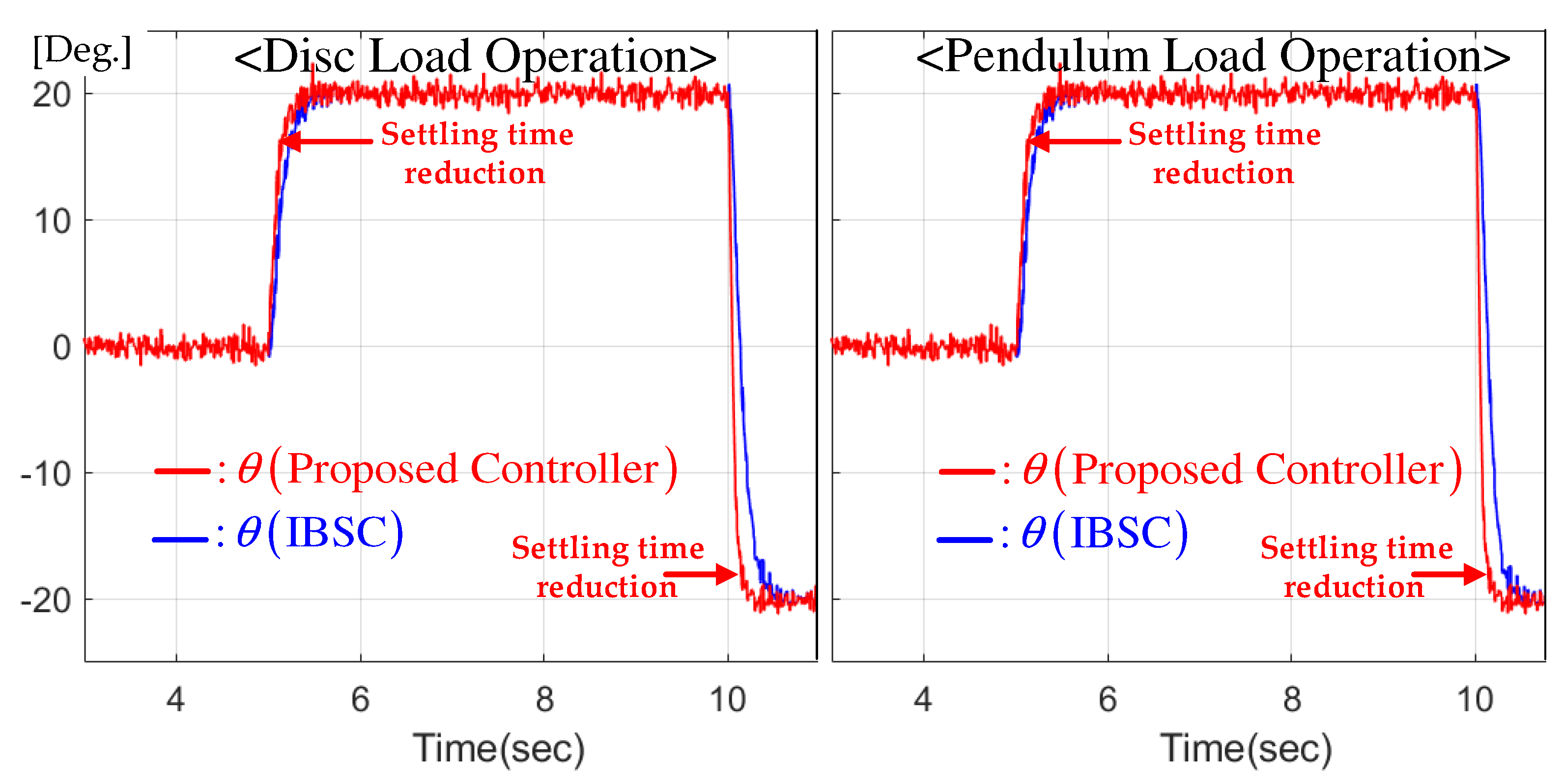
Figure 4.
Position feedback gain responses for disc and pendulum loads.
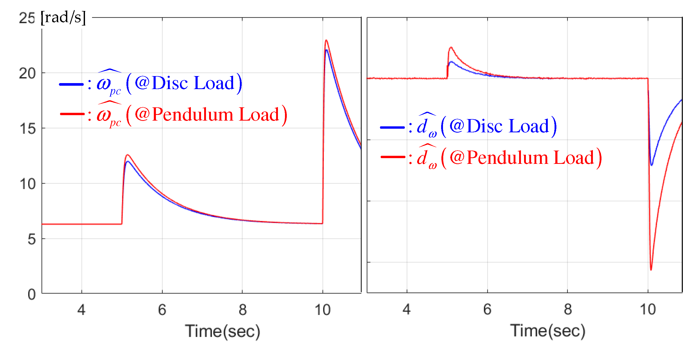
Figure 5.
Speed and angular velocity observer error responses for disc and pendulum loads.

Figure 6.
Sinusoidal reference tracking performance comparison for pendulum load.
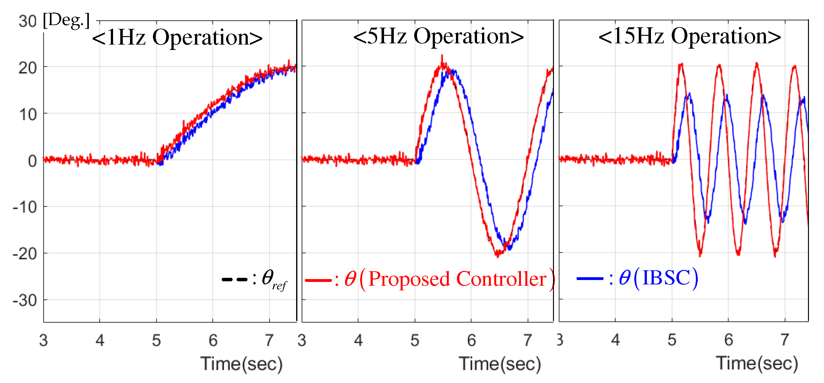
Figure 7.
Comparison of regulation performance for disc and pendulum loads.

Figure 8.
Stator current responses under regulation tasks for disc and pendulum loads.

Publisher’s Note: MDPI stays neutral with regard to jurisdictional claims in published maps and institutional affiliations. |
© 2021 by the authors. Licensee MDPI, Basel, Switzerland. This article is an open access article distributed under the terms and conditions of the Creative Commons Attribution (CC BY) license (https://creativecommons.org/licenses/by/4.0/).
Share and Cite
MDPI and ACS Style
You, S.H.; Kim, S.-K.; Choi, H.D. Output-Feedback Position Tracking Servo System with Feedback Gain Learning Mechanism via Order-Reduction Speed-Error-Stabilization Approach. Actuators 2021, 10, 324. https://doi.org/10.3390/act10120324
AMA Style
You SH, Kim S-K, Choi HD. Output-Feedback Position Tracking Servo System with Feedback Gain Learning Mechanism via Order-Reduction Speed-Error-Stabilization Approach. Actuators. 2021; 10(12):324. https://doi.org/10.3390/act10120324
Chicago/Turabian StyleYou, Sung Hyun, Seok-Kyoon Kim, and Hyun Duck Choi. 2021. "Output-Feedback Position Tracking Servo System with Feedback Gain Learning Mechanism via Order-Reduction Speed-Error-Stabilization Approach" Actuators 10, no. 12: 324. https://doi.org/10.3390/act10120324
Note that from the first issue of 2016, this journal uses article numbers instead of page numbers. See further details here.