Method to Integrate Radiant Cooling with Hybrid Ventilation to Improve Energy Efficiency and Avoid Condensation in Hot, Humid Environments


Department of Architecture, King Abdulaziz University, Jeddah 21589, Saudi Arabia
Buildings 2018, 8(5), 69; https://doi.org/10.3390/buildings8050069
Submission received: 3 April 2018
/
Revised: 23 April 2018
/
Accepted: 1 May 2018
/
Published: 8 May 2018
Abstract
:Although radiant cooling is considerably more efficient than conventional all-air room cooling systems, the potential for its application in warm humid regions is limited, owing to the increased risk of condensation by opened windows or unsealed openings in the building envelope. Having constantly closed windows and mechanical ventilation in such a climate needs to significantly dehumidify outdoor air to avoid the risk of condensation. The present study examines the effects of coupling hybrid ventilation (window and mechanical) with radiant cooling during periods of acceptable outside air temperature. An optimization method that increases energy efficiency and maximizes risk-free window opening potential in the critical seasons (summer and autumn) is developed and applied. IDA-ICE software is used to conduct dynamic thermal simulations of a typical studio classroom model, for which different cases and conditions are investigated. Different cooling and ventilation scenarios and control strategies are integrated and examined. Potentials and limitations can be noted between the various cases. Moreover, analyses using ANSYS-CFX as well as other tools are developed for verification and to assess the impact of the suggested optimization method on the indoor air and user comfort. The findings indicate great potential for the proposed solution in lowering the energy demand considerably and providing condensation-risk-free window opening potential.
1. Introduction
1.1. Advantages and Limitations of Coupling Hybrid Ventilation with Radiant Cooling
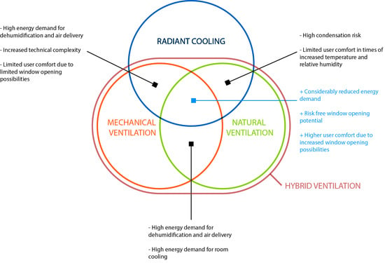
Considering the currently increasing energy costs and growing ecological concerns, hybrid ventilation systems that integrate natural ventilation solutions with mechanical ventilation are effective for achieving user comfort with less energy and technical complexity [1,2,3]. Increased user comfort has been reported in association with window opening potential and user control over natural ventilation [4,5]. Using conventional (all-air) cooling systems, cooling loads are extracted via the circulation of large volumes of cooled or conditioned air. This approach not only demands large quantities of energy, but also requires considerable space for the ducts and technical equipment with respect to the circulated volume of air. This is essentially because, in the cooling case for instance, the entire room needs to be cooled by air to achieve the desired air and target operating temperatures. One efficient cooling method is an air–water method that involves a combination of mechanical ventilation of cooled air and radiant cooling via chilled surfaces incorporated in the ceiling, floor, or walls. Concerning such a system, the supplied and conditioned volume of air is minimized to the amount required to maintain a certain indoor air quality, which is often related to the accumulated CO2 level in the room. Different from conventional (all-air) air-conditioning systems, the air–water approach is sensible because the specific heat capacity of water is higher than that of air, which makes it 4000 times more efficient for energy transport [6]. Feustel and Stetiu [7] claim that 40% energy savings could be attained using radiant cooling compared to conventional air-conditioning approaches. In such systems water circulates through pipes that are in contact with a surface. A more efficient method would perhaps include hybrid ventilation to make use of possible passive techniques that involve window ventilation, mechanical ventilation, and radiant cooling. The diagram in Figure 1 summarizes the concept of the proposed system of hybrid ventilation coupled with radiant cooling. It also lists the limitations of other coupling possibilities that involve only two of the three components.
Whereas in the first all-air cooling, heat is extracted via forced air convection, in radiant cooling, the water-cooled surface extracts heat from the room through both radiation and convection. Additionally, radiant cooling does not require a large temperature difference between the desired room temperature and the surface temperature; it can operate with a temperature difference as small as 2–4 K [8], which is significant for energy conservation. This is because the comfort temperature of the room can be set higher than in conventional air-conditioning systems, as a large portion of the heat generated by human bodies is absorbed via radiant heat exchange with the cooling panel. Although another study by Stetiu [9] asserts that an average of 30% savings can be achieved in the United States via radiant cooling, one of the significant challenges for this system relates to its application in hot, humid climates, owing to potential risks of condensation that typically occur via the intake of warm humid air through infiltration or large openings in the building. Fundamentally, condensation on the cooling surface occurs if the surface temperature is below the dewpoint temperature (Td) of the air. This essentially limits the potential of hybrid ventilation using window openings, as condensation is often associated with mold formation and the deterioration of indoor environmental quality.
Several studies have addressed eliminating the condensation problem in radiant cooling systems from different points of view [10,11,12,13,14,15]. Rhee and Kim [16] conducted a wide-ranging literature review on the issues related to radiant cooling and the challenges associated with its application. Among 540 selected papers, 68 were chosen for detailed analysis. The results indicate great potential for radiant cooling for energy efficiency and improved thermal comfort. However, the authors suggest further studies to overcome the limitations and challenges associated with specific climates, building types, and control systems. The following are methods presented in multiple research works to deal with the problem of condensation. Chiang et al. found that an increased air supply temperature (Tsup) of 24 °C saves 13.2% for the chiller and 8% for the entire cooling system [17]. Although this approach is useful from an energy saving perspective, the condensation risk may increase if the supplied air contains a high amount of moisture that is not adequately extracted via dehumidification, which involves cooling the air below its Td; i.e., latent cooling. Vangtook and Chirarattananon [10] found that maintaining the surface temperature at 25 °C is sufficient to avoid condensation under certain conditions. The limitation of this approach is that it is more suitable for spaces with significantly low heat gains. The research also suggests using cooling water, generated by a cooling tower, for radiant cooling and mechanical ventilation. Zhang and Niu [18] assert that during the day, air dehumidifiers and mechanical ventilation should be operated, starting one hour before using a radiant cooling system to avoid condensation, which clearly indicates a limited capacity for window ventilation. A comparison between an underfloor air cooling system and a hybrid ventilation system using cross-ventilation was conducted by Song and Kato [12], who claim that the latter is considerably more energy efficient. The study describes a method to remove condensation on the vertical radiation panels of the hybrid ventilation system by incorporating a drain pan in the lower part of the panel, but this requires an extra plumbing system. Similarly, Hindrichs and Daniels [14] suggest using large-scale cooling radiators, in the form of pipes that simultaneously work as wind barriers and dehumidifiers, for a project in Abu Dhabi. This idea extends the potential of hybrid ventilation to be applied in outdoor spaces. Another concept to increase the potential of radiant cooling was introduced by Seo et al. [13]: they suggest coupling outdoor air cooling and radiant floor cooling by integrating a ventilation device in the facade that facilitates dedicated ventilation, dehumidification, and outdoor air cooling. The main feature of the system is that it minimizes the need to cool outdoor air and helps remove moisture from the recirculated indoor air, resulting in 20% savings with respect to conventional radiant cooling. Yet, the system requires an extra decentralized ventilation device to be incorporated into the building envelope, which has limitations from flexibility and architectural design perspectives.
Other ideas to prevent condensation were discussed by Hong et al. [15]. The authors conclude that a dehumidification ventilation system is essential to prevent condensation in hot, humid climates. Moreover, it is always recommended that a building management system (BMS) have condensation control strategies. As suggested by Seo et al. [13], the water supply should be limited and controlled to maintain the surface temperature at least 2 K above Td. Siegenthaler notes [19] that the recommended safety margin should be between 2 and 4 K. This is understandable, considering sudden fluctuations in indoor temperature and thermal loads, particularly in spaces with a large number of users, such as classrooms.
Since cross-ventilation is essential to discharge heat from a building, providing continuous window ventilation while radiant cooling is in operation was the focus of Song and Kato [12]. Cross-ventilation is also fundamental for improving thermal sensation under hot, humid conditions. Regarding traditional buildings in hot, humid cities such as Jeddah, Saudi Arabia, interesting lessons can be learned. The high thermal mass of the massive structures provides a passive form of radiant cooling. Since buildings were optimized for natural cross-ventilation, traditional structures in Historical Jeddah present an example of coupled radiant cooling and ventilation. This method is also described by Konya [20]. Although some researchers tend to solve the problem of condensation after its occurrence through drainage systems, others suggest that the temperature of the cooling surface be controlled to prevent it. However, within the scope of this research, it is found that there is a clear correlation between window opening modes, radiant cooling surface temperature, and the Tsup of the mechanical ventilation system. Mechanical ventilation cannot always be avoided in classrooms if the indoor air quality is to be maintained. This is simply due to the fact that during periods when the outdoor temperature (Ta) is acceptable, the wind might be still, and air exchange might be limited. This provides solutions that keep the radiant cooling surface away from the risk of condensation. Therefore, solutions to avoid mold growth are out of the scope of this research. However, useful steps to overcome this issue are highlighted by [12,13].
1.2. Motivation
Air-conditioning is responsible for more than 70% of the nation’s electric energy consumption [14] in the rapidly developing and hot country of Saudi Arabia. Therefore, considering current changes in Saudi Arabian energy economics, it is important to rethink the way buildings are cooled. Building designers and planners need to clearly distinguish between cooling and air-conditioning for this to happen. Furthermore, effective planning of indoor climates should consider limiting the amount of conditioned and cooled outdoor air to a level essential for maintaining high indoor air quality and using radiant cooling to remove sensible heat loads. The market for radiant cooling is relatively limited in hot-humid climates, mainly due to fear of condensation [11]. This suggests room for research on methods to extend the feasibility and practical incorporation of such systems.
Educational facilities, including university buildings, are among the high energy consumers in Saudi Arabia. Recent data on the energy consumption of King Abdulaziz University in Jeddah in 2016 indicate an extremely high annual electrical energy demand. At least 40% of this energy is consumed for cooling, and the remainder includes the energy required for operating the HVAC systems. This suggests a potential for substantial energy savings by improving the cooling strategies and ventilation modes.
Additionally, there is growing evidence that natural ventilation of classrooms is essential for providing comfortable indoor air quality, which is significantly related to the performance, including the learning and working abilities, of the occupants [15,16,17,18]. The investigation conducted by Dhalluin and Limam [16] related the impact of natural ventilation to the seasons and building location, which extends its potential considerably. Their results indicate that, under given conditions, an automated window opening system controlled by the air temperature and lighting level is more effective in summer than in winter. However, relying less on mechanical ventilation is extremely important for energy saving and reducing maintenance and operational efforts. Moreover, the potential of window ventilation and its impact on energy efficiency was discussed by Bayoumi [18]. The study displays the sensitivity of the window opening grade using a window opening threshold temperature (WOT) of 25 °C. The spaces modeled contained an ideal cooler and no investigations related to condensation risk were conducted. However, despite its potential energy saving, considering radiant cooling and hybrid ventilation in the hot, humid climate of Jeddah poses challenges due to the risk of condensation that may take place if outdoor air is mixed with indoor air, for instance, by mechanical ventilation, while radiant cooling is active.
1.3. Novel Contributions of the Paper
The current approaches, from the literature review, in providing radiant cooling in hot-humid climates can be summarized as follows:
- Extreme dehumidification and dry air intake
- Limited supply of dehumidified air through façade-incorporated devices
- Increase the temperature of radiant cooling surface
- Vertical mounted radiant cooling surfaces and manual collection or extra drainage of condensate water
- Full operation of mechanical ventilation by increased relative humidity
Although different methods to increase energy efficiency and avoid condensation have been discussed in the reviewed research works, none of the provided solutions have directly considered the window opening potential. The coupling of natural window ventilation with radiant cooling is much more energy efficient than conventional air-conditioning [17]. However, this factor is crucial as it correlates with and significantly affects the Td of a room and increases the risk of condensation if other correlating factors are not considered in the planning and operation of the building. Furthermore, although one research work suggested a fixed Tsup of intermittent mechanical air supply to avoid condensation, other studies did not focus on this issue.
To the best the author’s knowledge, this is the first study that addresses a method for integrating hybrid ventilation with radiant cooling with respect to WOT, Ta, Tsup, Td, and ceiling surface temperature (Ts,c). The presented optimization method that generates a range of recommended Tsup is an additional contribution that helps maximize the condensation-risk-free window opening potential (RF-WOPot) with minimum possible energy demand for outdoor air cooling used with mechanical ventilation. While the investigated case is a classroom facility in the hot-humid climate of Jeddah, Saudi Arabia, the presented method can be applied under other conditions to other locations to assess the feasibility of considering such a system during the early design and planning stages of a building’s technical outfitting.
2. Methods
2.1. Thermal Simulation Framework
2.1.1. Room-Specific Parameters
An architectural studio classroom in the Faculty of Environmental Design, King Abdulaziz University, was selected as a case study for this analysis. This room was selected mainly because architecture students tend to work long hours at school to make effective use of the open hours. Additionally, such a classroom has the potential to replace existing suspended ceiling panels with radiant cooling surfaces. Recent market developments and studies on capillary mats indicate great potential for integration of suspended ceilings with effective heat transport and temperature uniformity [19,20,21].
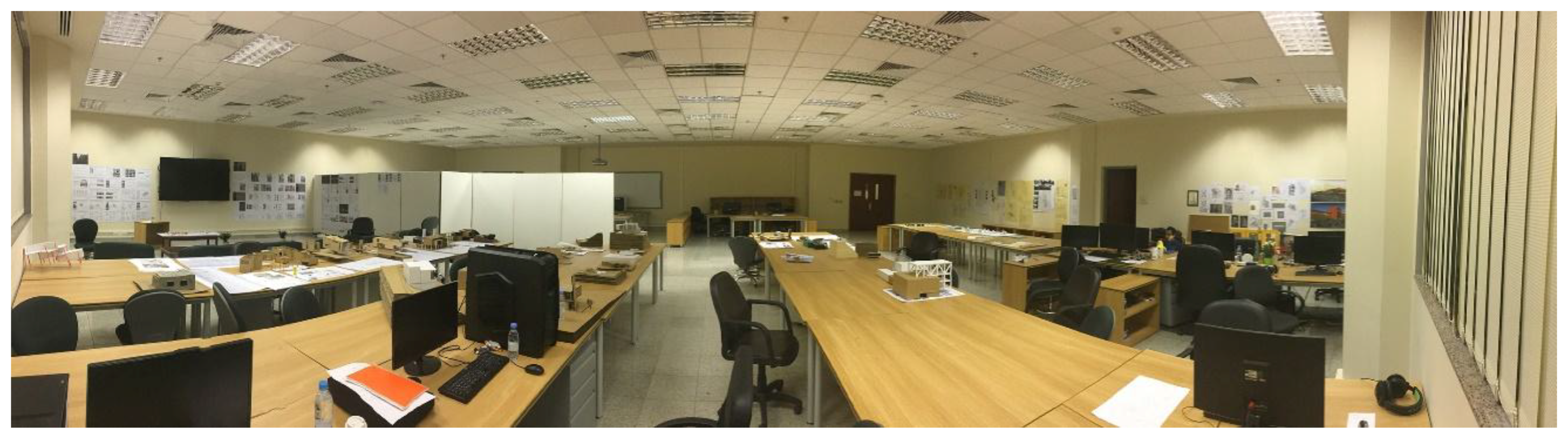
The selected studio-classroom had an area of 305.2 m2 and a ceiling height of 4 m. It was equipped with an all-air air-conditioning system. The orientation of the studio-classroom was to the west, with three large non-operable windows occupying 40% of the facade.
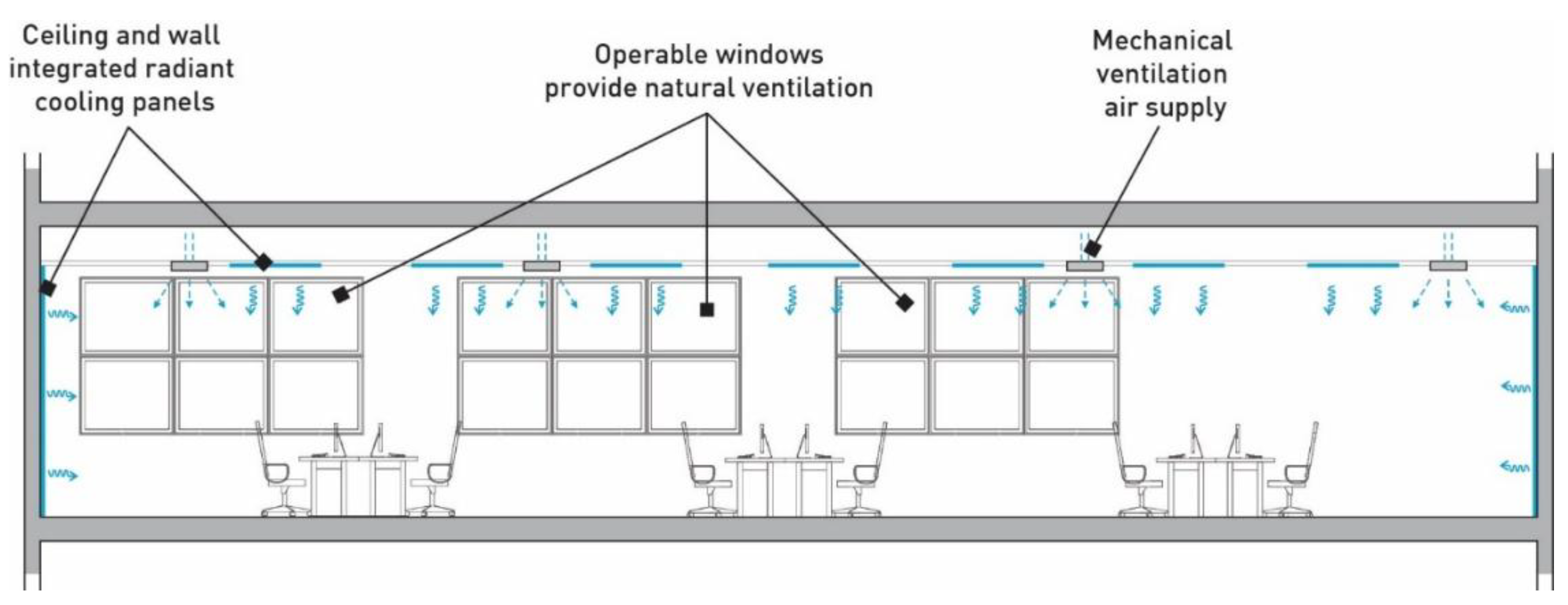
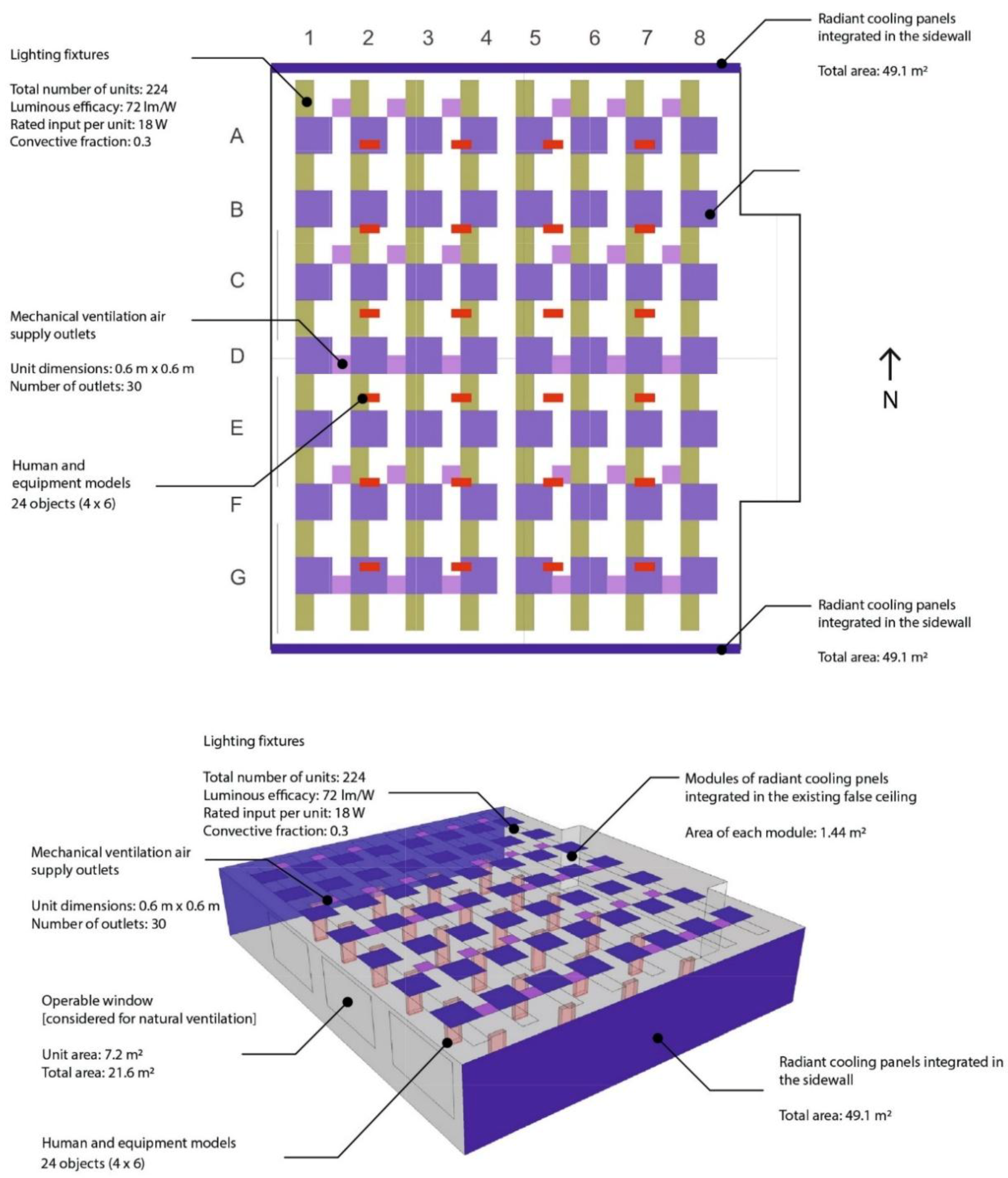
Figure 2 shows a wide-angle interior view of the case-study classroom. Figure 3 illustrates the elements of the cooling and hybrid ventilation concept. Besides the operable windows located on the western side, mechanical ventilation provides cooled and dehumidified air as much as needed to maintain a certain level of indoor air and environmental quality. According to the given framework of the classroom, the most appropriate places to integrate radiant cooling panels are the existing false ceiling and the side walls located at the northern and southern sides of the room.
The simulation model can be seen in Figure 4. The classroom has an area of 305.2 m2 and a volume of 1221 m3. The software IDA-ICE 4.7.1 is used for conducting the thermal simulations. This software package can conduct dynamic thermal simulations to evaluate the performance of the building or part of it. The calculations are based on the annual hourly climate data of the selected location. The design data files are provided by the simulation software and based on ASHRAE Fundamentals 2013. While the dynamic simulation produces the results for 8760 h, for easier understanding the results are averaged to be representative of four typical days for each of the four seasons. This means each of the 24 h presents the mean values of climate conditions across the season. Additionally, the included large HVAC database in the software contains different types of radiant cooling systems that can be incorporated into the simulation models. The modelling includes the thermal conditions of the classroom as well as the associated parameters of the HVAC system that comprise the air supply temperature and the resulting electric energy demand for cooling. The Coefficient of Performance (COP) of the chiller has been set to 3.0. Additionally, the program enables the development of different control systems that can be applied to windows, building services, and many other components. More information on the selected software is available elsewhere [22,23]. The existing condition was modeled as Case (1) to estimate its energy consumption for cooling. Case (2) had further developments implemented to establish a new reference case, which included radiant cooling, to be used in comparison with further investigations. The temperature of the radiant cooling surface was automatically controlled with respect to indoor air temperature (Ti). The thermal properties of the facade were altered to allow more daylight penetration. An external screen, to be drawn when solar radiation reached 100 W/m2, was incorporated. Table 1 outlines the simulation conditions of both cases. The daily schedule of the simulation model included an occupant availability factor of 1.0 from 10:00 to 16:00, and 0.5 from 08:00 to 10:00 and 16:00 to 22:00 on weekdays, and an availability factor of 0.5 from 08:00 to 22:00 on the weekends. Data from Figure 5 represents a calculation for the entire year.
The room was assumed to contain 24 occupants, who each had a computer with an average emission value of 75 W/unit. The rated input of the installed lighting was approximately 13 W/m2, with a luminous efficacy of 75 lm/W and a convection fraction of 0.3.
Outdoor air infiltration affects the quality of indoor air considerably and, thus, changes the overall setting of the indoor air volume including the dewpoint temperature. The modeling of outdoor infiltration was considered in the dynamic simulation parameters, in the model, 0.5 ACH at a pressure difference of 50 Pa. The infiltration rate was dynamic and associated with wind driven flow.
2.1.2. Climate Characteristics
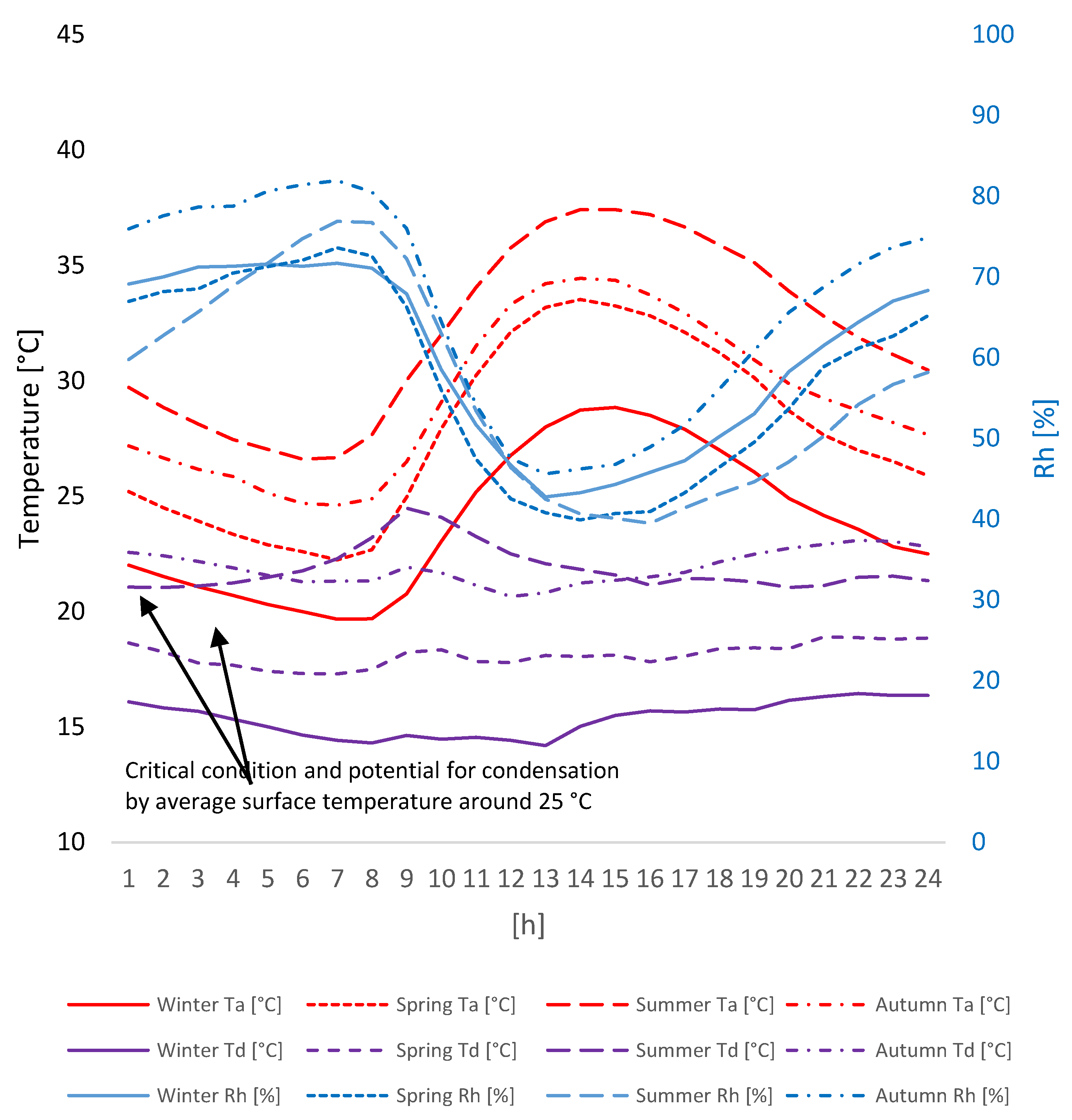
It was important to highlight the main climate characteristics of the location of the study for the next analyses. Figure 4 has the primary axis represent Ta (red curves) and Td (purple curves) for an average day in each season. The corresponding relative humidity (Rh) (blue curves) is displayed on the secondary axis. The calculation of the Td was done using the August–Roche–Magnus approximation [24,25] presented in Equation (1), where a = 17.625 and b = 243.04:
Figure 5 indicates the potential risk of condensation if the surface temperature drops below 25 °C and a window is opened, which could occur in summer or in autumn. During summer, the Ta is rarely less than 32 °C during working and studying hours, and the potential for night ventilation is limited owing to the small temperature difference between day and night. Therefore, it is sensible to consider keeping the windows closed in summer if no window opening control system is available. Under these conditions, the preliminary climate investigation does not indicate a condensation risk in winter or in spring, however, the problem remains in autumn.
2.1.3. Thermal Simulation Model
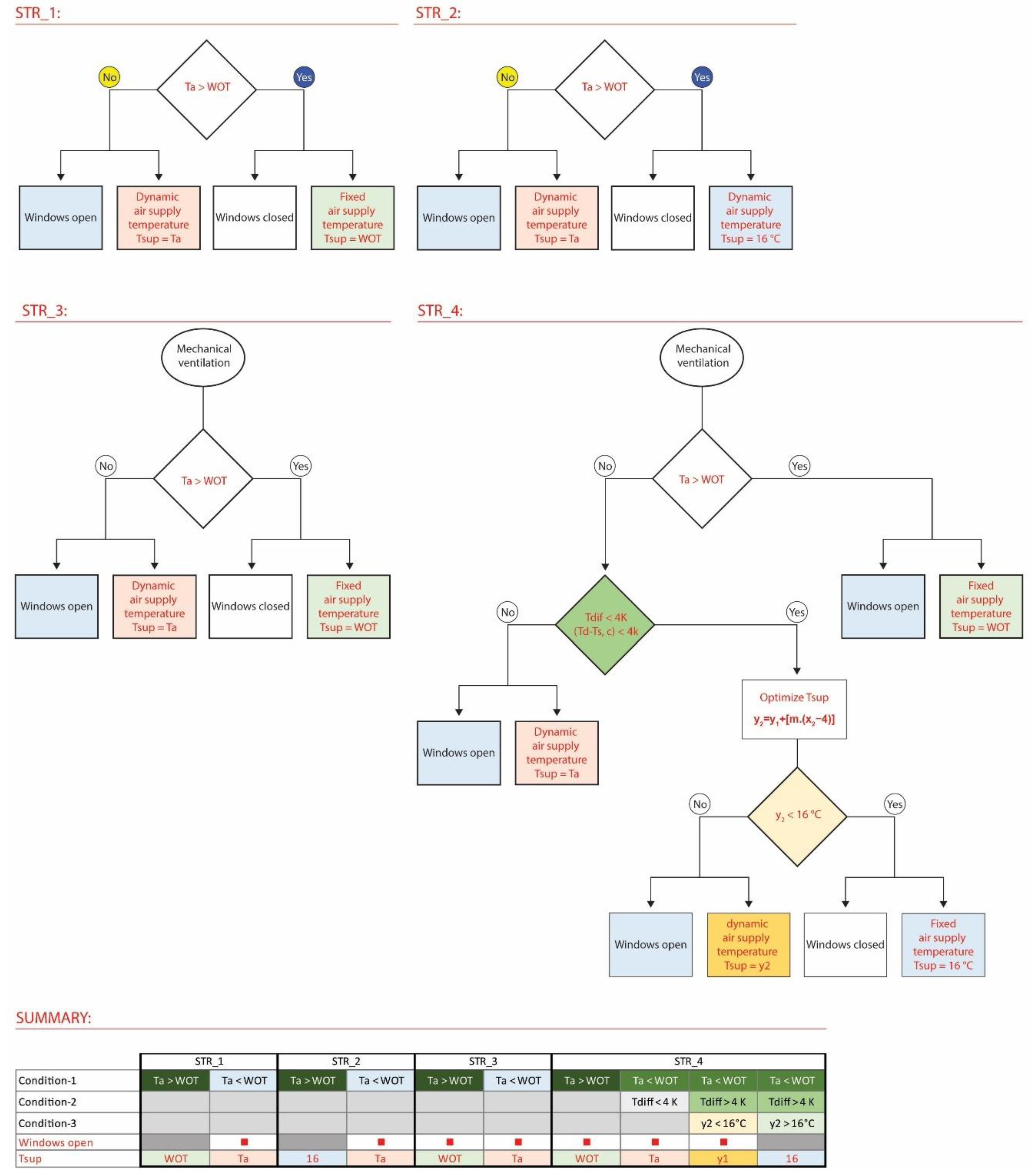
Six investigation cases were developed and simulated. Table 1 outlines the simulation cases and framework. As discussed above, Case (1) and Case (2) refer to the base models, in which windows were never opened. Moreover, while Case (1) represents the actual reference case, Case (2) includes slight developments in the façade configurations and room set temperature. Generally, a WOT of 28 °C had been set in the simulation models of the rest of the cases. The “d” in Table 1 stands for dynamic control modes, where Tsup follows a specific routine. Four control strategies were developed and set to control the intake air using mechanical ventilation with respect to Ta and WOT. Air was delivered via the air outlet located in the ceiling of the room and was required to maintain a satisfactory level of indoor air quality.
Figure 6 outlines the control strategies. STR_1 and STR_2 of Tsup used mechanical ventilation for the intake air, which was delivered via the air outlet located in the ceiling of the room and was required to maintain a satisfactory level of indoor air quality. Ta was assigned as Tsup and the window would open in both STR_1 and STR_2, if Ta was equal to or less than WOT. The window would close and WOT would be assigned as Tsup in STR_1, if Ta was higher than WOT. The same applied to STR_2, except that the Tsup was fixed at 16 °C if Ta was greater than WOT.
Other than the stated setting in Table 1, all the room parameters were fixed to ensure consistency in the simulation results. The intake volume of fresh air was set in association with the required air exchange rate to maintain adequate indoor air quality. Obviously, the performance of the users was affected by an increased level of CO2 concentration; the default threshold set in IDA-ICE for CO2 concentration to activate the fresh air supply was 1000 ppm. Heat dissipation and moisture generation by the occupants are essential issues that are calculated internally by IDA-ICE. This includes both sensible (dry) and latent (moist) heat emitted by the occupants. The resulting indoor relative humidity in the room is affected by the internally generated moisture by the occupants which also determines the Td in the room. This factor is obviously affected by opened windows and recalculated accordingly.
Further, Case (5) integrates a dynamic WOT that optimizes the WOT to achieve the maximum possible RF-WOPot. The model is explained in Figure 7. Moreover, in Case (6), a further optimization step was conducted and presented. Measures were taken in the simulation model to minimize the cooling load while keeping the maximum RF-WOPot. The risk of condensation was assessed by calculating the difference between the ceiling surface temperature Ts,c and the Td in the room while the windows were open. The mechanical ventilation was also active for indoor air quality control. The condensation risk arose if Tdif, which was the temperature difference between the Ts,c and the Td of the room air, was below the safety margin according to Equation (2). Within the scope of this research, Tdif values of 4 and 2 K were identified as minimal and considerable risk, respectively. Moreover, the Tsup played an important role in changing the Td of the indoor air, which obviously affected Tdif.
Furthermore, it is important to note that the different air supply temperatures, ranging from 16 to 32 °C, could lead to various levels of thermal comfort and air distribution patterns.
2.2. Optimization of the Air Supply Temperature to Avoid Condensation Risk and to Achieve the Minimum Cooling Load
As the air supply was mainly used for maintaining a certain level of indoor air quality, the temperature at the air intake (represented as Tsup) was a decisive parameter that affected the cooling load considerably. However, in hybrid ventilation systems, in which window ventilation was considered under certain conditions, and for energy saving purposes, it was not always needed to set Tsup at 16 °C as for STR_2. The main difference between STR_2 and STR_3 was that the windows in the latter were open. This is applied in Case (6) and explained in Figure 8.
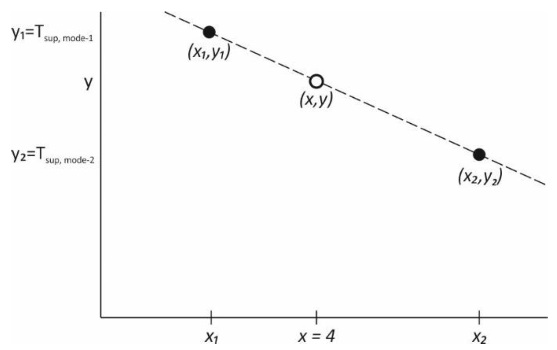
Obviously, relying on STR_1 completely where Tsup was equivalent to Ta under certain conditions, such as in Case (4), caused condensation during periods of high Td of outdoor air. Air was delivered unconditioned and might have contained a high amount of moisture, which condensed on cold surfaces. This suggested the development of a new air supply strategy STR_4 that limited the amount of cooling of Tsup to an intermediate level between the two extreme approaches mentioned, and which did not exceed the required Tdif of 4 K. Since the optimum Tsup was between Tsup of STR_1 y1 and Tsup of STR_2 y2, using the point–slope form of straight-line equations [26], the optimum Tsup y in Equation (3) solved for x = 4, which represented the limit for Tdif. The variable m represents the slope in Equation (4):
where x1 and x2 indicated Tdif of the cases of STR_1 and STR_2, respectively, were applied. Figure 7 explains the implemented method to determine the optimum Tsup for Case (5) and Case (6).
Equations (3) and (4) had the optimum Tsup calculated as follows:
This also means, that under the application of STR_4 where Ta was higher than WOT, no condensation was expected. This is because the Tsup was modified according to the blue and brown curves in Figure 8. While the Tsup was reduced to the level where the Td of 4 K was maintained, it was not extremely reduced to reach 16 °C, which would have caused the unnecessary consumption of cooling energy. The diagram also presents the resulting Td in the room after mixing its air with the newly supplied air from both window and mechanical ventilation.
2.3. Verification of Generated Findings
The simulation results were calculated using the dynamic thermal simulation software IDA-ICE, yet it was also important to analyze the airflow, its impact on user comfort, and the radiant cooling panels. Particularly, the room air temperature, with such a mixed ventilation mode, needed to be in stable and comfortable ranges. Further, the temperature of the cooling panels had to remain above the Td of the room air. Although experimental fluid dynamics tests and, especially, wind tunnel simulations are widely accepted in the scientific and engineering community as the most reliable validation methods, recent advances in computational fluid dynamics (CFD) simulations offer great potential as they have shown very accurate and comparable results to real-world conditions within reasonable bounds of errors [27]. The limitations of computer simulation models have been discussed and pointed out by many scholars, with respect to many software packages [28,29]. Therefore, the current investigation included the basic simulations using IDA-ICE. The outcomes were verified with the aid of CFD analysis with a focus on summer and autumn due to their critical conditions. Further verification using a Hx-diagram and an online tool was considered.
2.3.1. Steady-State CFD Simulations
To develop a better understanding of the results generated by IDA-ICE, CFD simulations were conducted using the relevant parameters of the thermal simulation model. The classroom model depicted in Figure 4 was used in the CFD simulation. The aim was to validate the results by replicating the model in another simulation environment. Within the scope of this study, steady-state thermal CFD simulations using ANSYS-CFX were used to validate the results of the thermal simulations. Basically, the CFD software solves the partial differential equations governing a flow field to predict the velocities, pressures, and temperatures at all points in the field via discretization process using finite volume techniques they are also called Navier–Stokes equations. Moreover, the CFD are considered a powerful design tool that model complicated flow situations. However, it is crucial to consider the main limitations and uncertainties that are according to Tamura et al. [30,31,32] attributed to the turbulence model, calculation grid, and boundary conditions. The frameworks of both aspects within the scope of this study are included in the following text. The averaged Navier–Stokes equations can be expressed in the following equations.
Continuity equation:
Momentum conservation equation:
where is the sum of body forces, is the effective viscosity accounting for turbulence, and represents the modified pressure. Therefore, the left side of Equation (7) represents convection and the right side represents in sequence, pressure body forces, diffusion, and the momentum interaction between forces.
The set turbulence model was a standard . as it is widely used in engineering applications. The default medium turbulence intensity of (5%) was also set in both natural and mechanical ventilation inlet parameters. Stamou and Katsiris [32] performed an experimental verification study of a CFD model for indoor airflow and heat transfer. Several turbulent models in the CFD analysis were tested including the one used within the scope of this paper. They concluded that the standard model which is a semi-empirical model was able to generate acceptable predictions of the main qualitative features of the flow. Further, the layered type of temperature fields was also well predicted. Therefore, they asserted that it is possible to use these models for practical purposes. To describe the effect of turbulence, is replaced with in Equation (8), which is the turbulence viscosity. The modelling of is shown in Equation (9). The values of and are generated from the differential transport equations the describe the kinetic energy and turbulence dissipation rate, Equations (10) and (11) respectively. in Equation (12) depicts the turbulence production due to viscous forces. A full buoyancy model was used and is modelled according to Equation (13).
where , are empirical constants, with values 1.44, 1.92, 0.09, 1.0, 1.3, and 1.0 respectively.
During another benchmark experimental study in the subtropical climate of Taiwan by Chiang et al. [33] radiant cooling was combined with mechanical ventilation. A standard turbulence model was also used in their numerical part of the study, which is the case in this investigation. A remarkable improvement in thermal sensation (PMV within ±1.0) was reported even by increased Tsup of up to 24 °C. During this flow, the researchers noticed extremely uniform temperature distribution. Moreover, a P-1 radiation model was selected. The essential meshing parameters and their set values are shown in Table 2. No further modifications were implemented to the other default parameters given by the software. Additionally, RMS was set as a residual-type targeting 0.0001.
A single hour (09:00 AM) from the average day in the two most critical seasons (summer and autumn) was selected for the validation process. The optimum strategy in each season for maximum RF-WOPot was selected for the simulation. Table 3 outlines the basic input data. The aim of this step was to assess the practicality of the proposed approach in achieving a desired indoor temperature that was in the human comfort zone and in an acceptable margin of a maximum 2 K from the generated temperature of the thermal simulation. It was also important to observe the air temperature around the radiant cooling panels. Regarding the suggested hybrid ventilation and radiant cooling approach, the following indicators were observed within the scope of this CFD simulation: air velocity, air velocity distribution, air temperature, air temperature distribution, surface temperature of the radiant cooling panels, and finally, the predicted mean vote (PMV) according to the ASHRAE Standard 55 scale of thermal sensation.
Due to the critical conditions in summer and autumn, which are mainly attributed to the elevated relative humidity of outdoor air, the CFD simulation results for both seasons will be depicted in detail. The settings of the water vapor pressure for the PMV calculation included 2383 Pa, and 2412 Pa for summer and autumn respectively. They were calculated from the framework shown in Table 3. The calculation of the mean radiant temperature took place in the CFD software and was obviously affected be the varying surface temperatures of the radiant cooling panels. The set metabolic rate of the 24 occupants was 1.0 met (sedentary work) with which was ca. 58 W/m2 body surface with clothing factor of 0.55 clo according to ASHRAE Fundamentals [34]. Assuming a body surface area of 1.8 m2, ca. 104 W/person is generated. To consider the heat dissipation by occupants in the CFD analysis, heating panels to represent human models as per the dynamic simulations in IDA-ICE were installed in the room. The 24 human models were distributed in the room evenly following an order of (4 columns × 6 rows). The panels are highlighted in red in Figure 4. Additionally, each of them would be using a computer that generated 75 W. The total generated heat was 3600 W (104 W × 24 persons + 75 W × 24 persons). This means, each occupant generated 150 W.
2.3.2. Grid Independence Analysis
Research found in [33,35] presented a method to perform grid independence testing by doubling the number of cells. Subsequent to refining the grid size, a further simulation was run to verify the sufficiency of the previously set grid. Therefore, the indoor temperature was analyzed in the two grid Cases: (a) 132,398 cells (b) 2,530,469 cells. The latter case represented an increase in size by 2.08 times. The analysis included 58 points and the temperature values were found in good agreement and no deviation was noticed. The further simulations were limited to the grid Case (a) to save calculation time.
2.3.3. Investigating Condensation Risk
A large volume of outside air meets another volume of mechanically conditioned air in the suggested hybrid ventilation concept. While radiant cooling surfaces were activated, a condensation risk arose if the Tdif between the surface and the air was not within acceptable limits. Using a Mollier Hx-diagram, each condition was analyzed and illustrated to determine the resulting Td of the mixed volumes. Next, Tdif will be compared with the previously generated results using the thermal simulation software IDA-ICE.
3. Results and Discussion
3.1. Impact of Radiant Cooling on the Current Condition (Closed Windows)
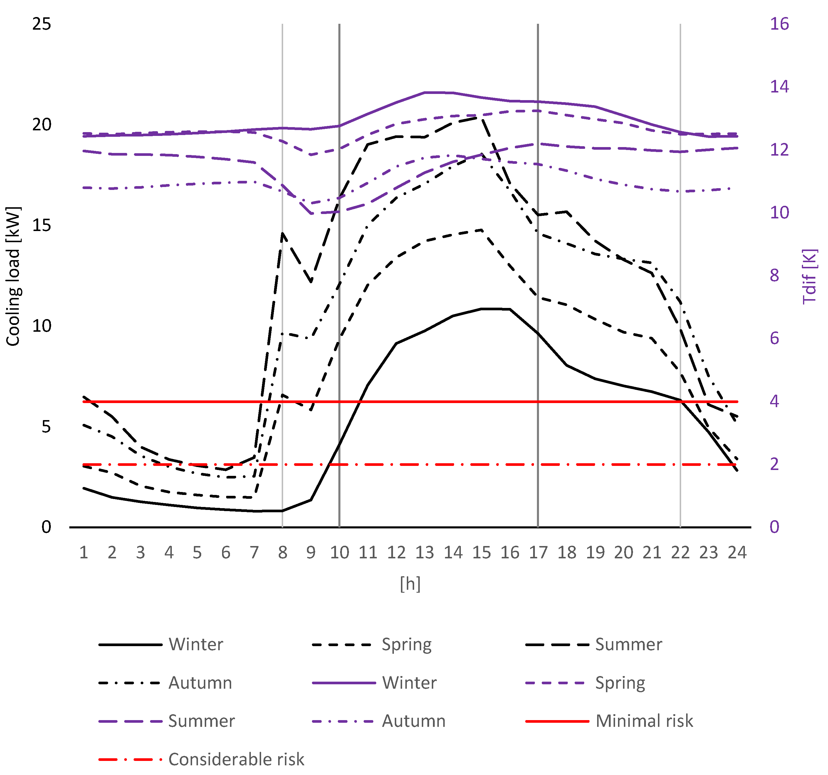
The simulation results for Case (1) (all-air) and Case (2) (air-water) indicated annual electric energy demand for the cooling of 422 kWh/m2·a and 84 kWh/m2·a, respectively. The current practice (Case (1)) assumed setpoint temperatures of 17–19 °C, which demanded high energy. Once setting the setpoint temperatures to 21–26 °C in Case (2) besides other enhancements in the façade setup, a radiant cooling arrangement with a cooling capacity of 58 W/m2 was integrated into Case (2). The primary axis of Figure 9 presents the seasonal daily average cooling load for Case (2), and the secondary axis indicates the resulting Tdif. Substantial savings could be achieved and the annual energy demand of this enhanced model dropped to 92 kWh/m2·a.
According to Figure 9, a clear distance was maintained between the condensation risk line and the Tdif values in the developed base model, Case (2), in all four seasons. This indicates safe conditions for retrofitting classrooms with radiant cooling panels and mechanical ventilation, with dehumidification and constant Tsup of 16 °C. Achieving the safe conditions was possible in Cases 0–2, in which the windows were continuously closed, eliminating the risk of condensation. Despite the clear energy savings and the supplied fresh air by mechanical ventilation, limited user comfort was provided owing to the lack of window ventilation. Particularly, the operation of natural ventilation was a significant parameter that affected the level of user satisfaction with the space [36]. The constant Tsup was also energy-intensive, and methods to avoid both limitations are explored in the next sections.
3.2. Window Ventilation Potential and Impact of Air Supply Optimization
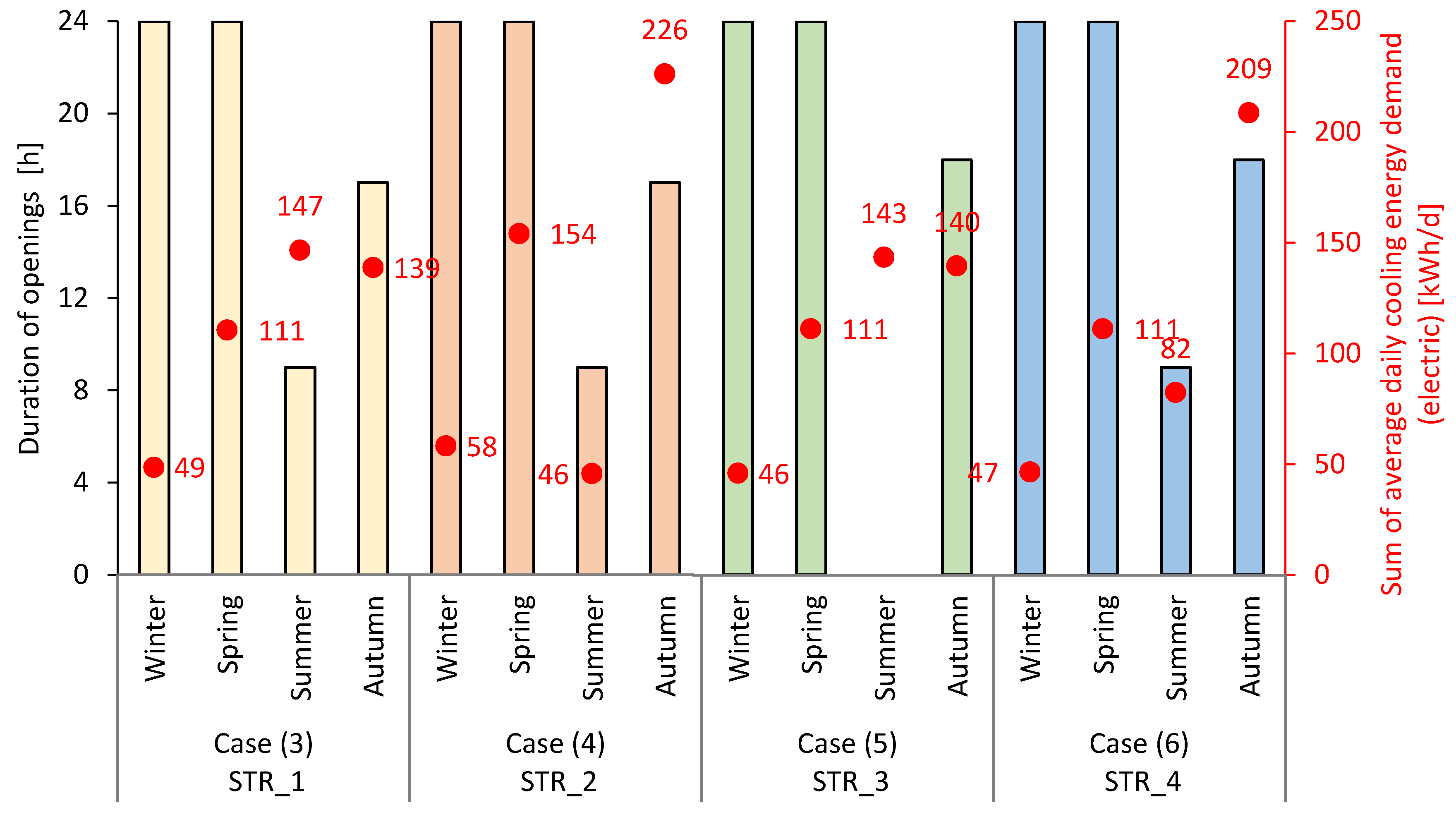
Figure 10 presents an overview of the window opening frequency (WOFreq) on an average day in each season (primary axis) against the average daily cooling energy demand (right axis); annual averages are indicated in orange. The unfilled columns refer to the WOFreq according to the WOTs, despite condensation risks. The filled columns represent the RF-WOPot where the minimal risk of condensation was totally avoidable (i.e., Tdif was higher than 4 K). The cooling load was relatively low in many cases where this condition was present. This is understandable where the Ta was in acceptable ranges and neither high energy for cooling nor dehumidification was required.
To discover the optimum cases that combined the best characteristics for each season, it was imperative to conduct a comparison addressing the relevant features of each case. The red circles in Figure 10 represent an overview of the daily electric cooling energy demand of the simulated cases. The data are displayed on the secondary axis. The annual data of each case is the sum of the seasonal daily average demands.
All simulations indicated a maximum RF-WOPot in winter, corresponding to 24 h/davg. A maximum achievable RF-WOPot of 24 h/davg in spring as well can be seen in the four presented Cases. The best conditions that included highest RF-WOPot in summer can be seen in Case (4), where WOT was set at 26 °C and STR_2 was used for Tsup, i.e., 16 °C. Furthermore, Case (4) also provided the best solution in terms of lowest energy demand for cooling. The best case from the same point of view in autumn was Case (6) according to the diagram. It satisfied lowest cooling energy demand per day (209 kWh/d) by highest RF-WOPot (18 h/d). Clearly, the absolute lowest cooling energy demand per day was met by Case (3). However, this case demanded that windows should not be opened at all to reduce the need for the dehumidification of mechanically supplied air to keep the Tdif higher than or equal to 4 K. Therefore, Case (6) demanded slightly higher cooling energy. This is understandable, because more cooling energy for Tsup was required to avoid condensation that might arise owing to the increased window opening duration.
Interestingly, in summer, Case (6) indicated much less energy demand (82 kWh/d) than Case (3) (147 kWh/d), which had a close value of RF-WOPot. Thanks to the optimization strategy of Case (6), savings of approximately 44% between both cases could be achieved.
Obviously, it was important to keep the window ventilation option available within the realm of hybrid ventilation to increase the satisfaction of the users. Regarding classroom environments, this impact has been discussed in detail by [16,17,18,37]. Following that, a comparison based on the seasonal average daily cooling demand was conducted to determine the cases that included the best qualities of both RF-WOPot and cooling demand. Under these conditions, Table 4 outlines the best strategy for each season.
The main findings of the conducted analyses can be concluded by the following points:
- The recommended control strategies for maximum RF-WOPot are:
- ○
- Winter: STR_1
- ○
- Spring: STR_1
- ○
- Summer: STR_2
- ○
- Autumn: STR_4
- The recommended control strategies for lowest cooling energy demand are:
- ○
- Winter: STR_3, STR_4, STR_1 (close values!)
- ○
- Spring: STR_1, STR_3, STR_4 (close values!)
- ○
- Summer: STR_2
- ○
- Autumn: STR_1
- STR_4 works best in autumn where the lowest cooling load by maximum RF-WOPot is achieved
- The optimum strategy for summer is STR_2
3.3. Assessing the Condensation Risk that is Associated with Each Strategy
The results of simulation Cases (2)–(6) are illustrated in Figure 11. The primary axis refers to each Tdif. The secondary axis depicts the Ta. The condensation limits (red curves) are also shown. The results correspond to the results outlined in Figure 8 and Figure 10. It can be clearly seen that all cases in winter and spring lie in the safe zone, away from the condensation line. Cases (3) and (5) face condensation risk in summer and autumn. Evidently, all the other cases are safe from condensation over the entire year. The gray curve in Figure 11 refers to Case (2), suggesting that the risk of condensation is minimized because window ventilation is not activated at all.
Especially in summer and spring Figure 11 indicates that the risk of condensation correlates with Ta when the windows are open (i.e., Ta < 28 °C). This is due to the increased temperature that affects the Td of the air flowing through the windows. Here, users have two options: close the windows and rely on mechanical ventilation or keep the windows open and mix the fresh air that enters through the windows with cooled dry air via mechanical ventilation. This is the scenario in which air cooling and especially dehumidification need to be optimized to eliminate unnecessary energy consumption.
Although the Tdif values for Cases (4) and (5) are presented Figure 11, it is important to relate them to the corresponding Tsup that was not optimized. The most striking result is the optimized Tsup curve of Case (6). According to the diagram, the curve is not located in the zone of considerable risk during daytime in summer, and during the night, early morning, and evening in autumn.
Moreover, the application of STR_4 in summer and autumn—presented in Case (6)—helps generate an energy-efficient, condensation-risk-free (air–water) cooling approach that effectively integrates window ventilation and radiant cooling. It is also important to consider such optimization methods of Tsup control, even though windows are closed, because infiltration causes temperature fluctuations and the condensation risk might increase again.
3.4. Comparison of Presented Strategies Against Reference Case
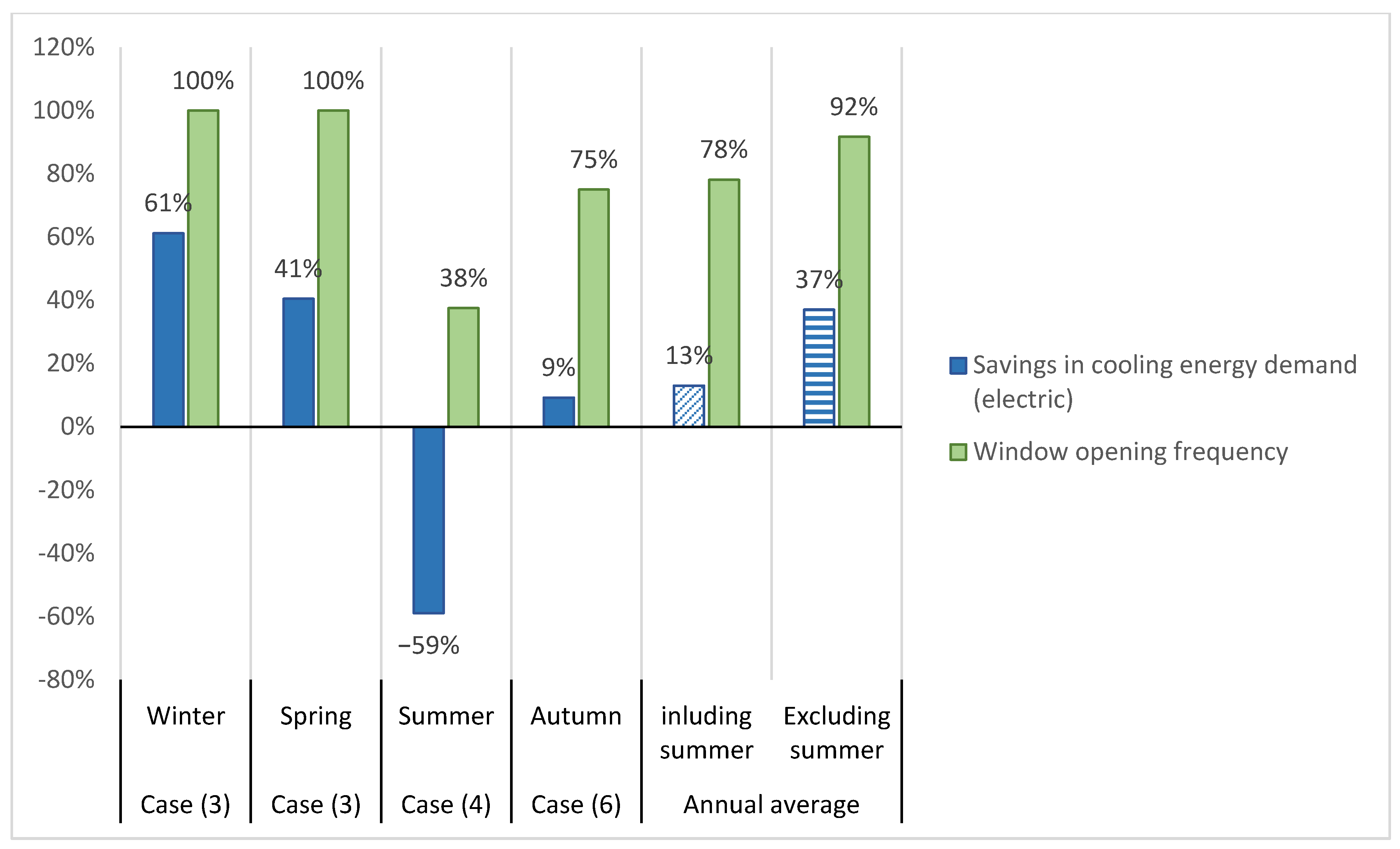
Having considered Case (1) as the base case that reflects today’s conventional practice, Case (2) represents a model that includes slight enhancements in the façade configurations, however, it still represents the all-air cooling approach. Therefore, it is useful to assess the energy savings in percentages in the presented strategies against the reference Case (2). Limitations are apparent in summer and autumn, owing to the increased Ta and Td.
Figure 12 provides a comparison of the best cases presented in Table 4 against the enhanced reference Case (2). According to the diagram, substantial savings can be achieved in winter, spring, and autumn. While the basic advantage of the suggested strategies lies in the maximized RF-WOPot, elevated energy demand for cooling can be seen in summer due to the increased required effort for dehumidification of Tsup to reduce Td in the room and keep it above the values of condensation risks. However, in this case, it is up to the users to decide whether windows should be opened in summer—under the given conditions—for improved room quality, or not. The average annual savings in the first option is in hatched diagonal blue lines. The latter option is in hatched horizontal blue lines.
3.5. CFD Simulations for Summer and Autumn Framework
The suggested hybrid ventilation setup involves mixing mechanically supplied air with naturally supplied air via window openings. Therefore, it is imperative to simulate the final effect of the mixed air volumes on the overall condition of the room. The following diagrams, Figure 13 and Figure 14, depict the result of conditions at 09:00 AM for the best cases according to Table 4, in the most critical seasons (summer and autumn), which are shown in the Cases (4) and (6) of Figure 11, respectively. Subsequently, the change in temperature in relation to volumes of the mixed air in each season at the selected time, as well as the corresponding Ts,c of the radiant cooling panels, are illustrated in the Mollier Hx-diagram afterwards. Table 3 provided the basis for the data input for both the CFD simulation and the Hx-Diagram.
The images in Figure 13 represent the conditions in summer of Case (4) after the application of STR_2. The image number 1 in Figure 13 depicts the surface temperature of the radiant cooling panels under the input conditions that are shown in Table 3. It is clear that the dominating Ts,c was between 24–25 °C. The temperature dropped on the sides of some panels due to the mechanically supplied cold air from the outlets located next to the radiant cooling panels. The temperature of the supplied air was 19.3 °C. Obviously, there was no risk of condensation in this case as the moving air in these zones had been dehumidified already. Once it touched the warm part of the surface, its temperature increased, and it absorbed moisture. Yet, no condensation was expected as the Ts,c was higher than the Td of the air.
The upper-left image in the simulation results shown in Figure 13 presents the air temperature distribution on a horizontal slice at a 1.5 m height. The diagram to the bottom represents the same data on Slice A-A. The location of the slice is marked on the upper left image. The air velocity distribution can be seen on the horizontal slice (top-right) and the vertical slice (bottom-right). Additionally, the location of the ceiling- and wall-integrated radiant cooling panels were marked on the 3-D images of the simulated classroom. The PMV distribution shown in image number 2 is around +0.3. This result is also in far from the result obtained from the dynamic simulation, which indicated an average PMV of 0.5. The average values are located around the neutral level on the scale of thermal sensation.
According to the results displayed on image number 3, A homogeneous temperature distribution can be seen. The average Ti lies between 24–25 °C. These values are in good agreement with the results obtained previously from the thermal simulation software IDA-ICE, which indicated an average Ti of 25.77 °C. Homogeneous distribution of Ti can be noticed in the vertical and horizontal slices. It is also important to note that the air velocity distribution presented in image number 4 was also within acceptable limits at human sitting and walking heights. It is also noteworthy that the increase in air velocity in such a warm humid condition helped improve thermal sensation under certain conditions [37,38]. Moreover, the resulting air mix not only helped avoid condensation in the hot, humid period of summer, but it also contributed to improving the temperature of outdoor air to reach acceptable levels for human comfort. The vertical temperature profile shown in image number 5 indicates an average temperature distribution in the range between 24–25 °C.
The levels of relative humidity were relatively high and as the outdoor temperature increased, the risk of condensation increases. According to the results shown in Figure 14 that represent the application of STR_4 in Case (6), the temperature distribution at human height is in the range between 24–25 °C. Image number 2 shows PMV values are approximately 0.2. While this suggests considerable correspondence between the CFD results and the previously generated thermal simulation results where the PMV equaled 0.5, it was assumed that the CFD simulation had considered the increased air velocity that contributed obviously to the enhancement of the thermal sensation. Ts,c remained around its initial values between 24–25 °C. The air velocity in the classroom reached a maximum of 0.14 m/s. Additionally, the air intake from the three available windows was considered in the CFD simulation model. The relatively high airflow mass via window ventilation of 0.47 kg/s allowed a large volume of unconditioned air to mix with the 0.18 kg/s of mechanically conditioned air.
3.6. Assessment of Condensation Risk Using Hx-Diagram
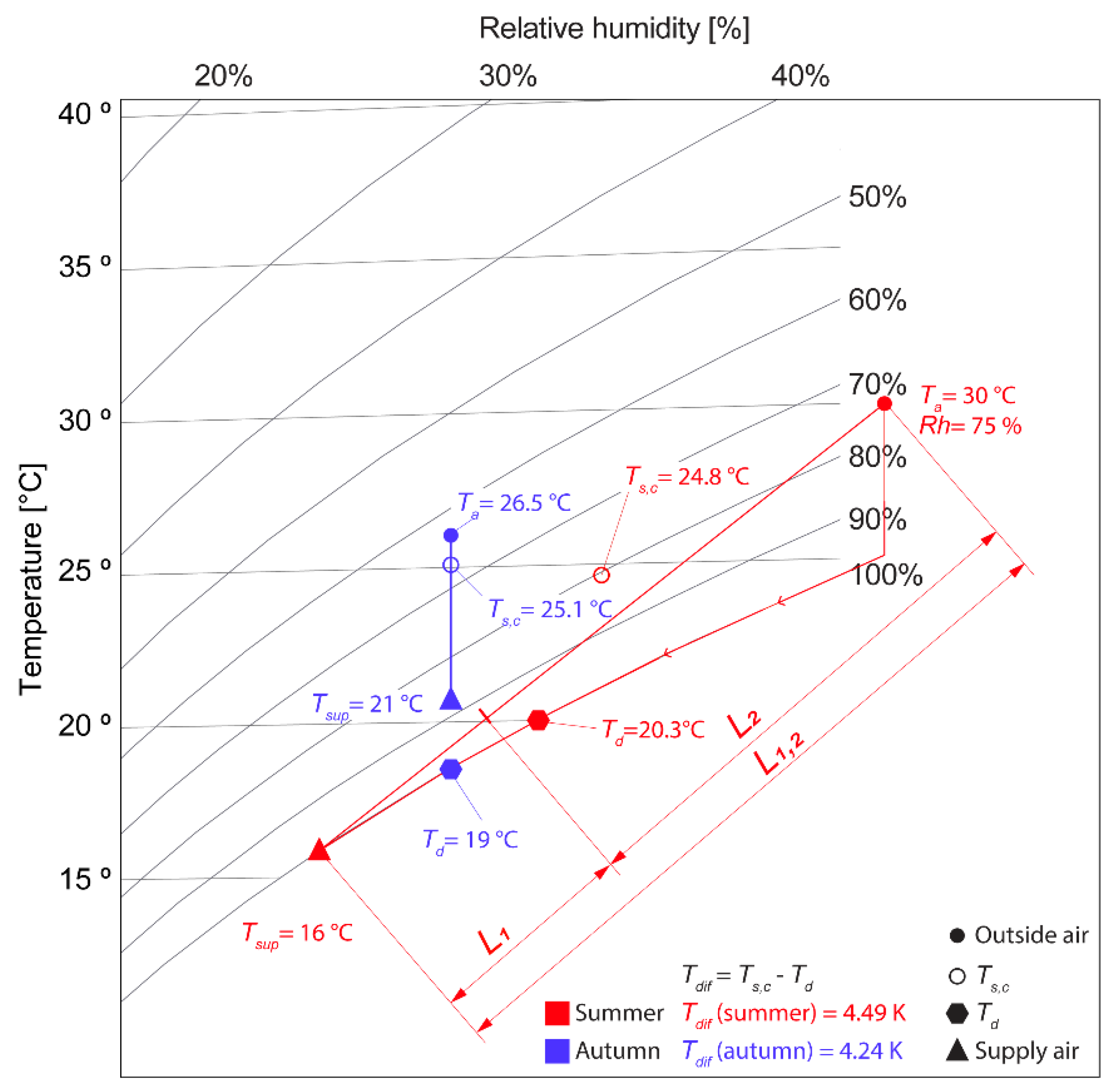
The Hx-diagram in Figure 15 outlines the conditions of the air/water mixtures at the selected time (09:00 AM) of each season, when hybrid ventilation was activated. Moreover, the shown data represent the results generated from the thermal simulation process of Cases (4) and (6) for summer and autumn respectively, in which Tsup was optimized to maximize RFWOPot. Similar to the CFD simulations, the presented data indicate the framework presented in Table 3. Clearly, the winter condition is not represented, as mechanical ventilation is not required. The conditions of spring, summer, and autumn are represented in purple, blue, and red respectively.
According to the diagram, sensible cooling is considered in spring and autumn when no change in specific humidity is required. However, the difference in temperature between Tsup and Ta in spring is trivial and the conditioned air is very similar to the outdoor air. During autumn, considerable reduction in the Ta can be seen to reach 20.81 °C. Since the dewpoint temperature of both cases, spring and autumn, is considerably below the Ts,c, no condensation risk is present.
Regarding the case of summer, a graphical approach of calculating the condition of the air mix was conducted. The aim was to determine the air mix between the naturally and mechanically supplied air. This is important to evaluate the risk of condensation in relation to Ts,c. Equation (14) presents the calculation method that indicates the results in proportion to the mass of each supplied air volume.
L1,2 indicates the total length between the two points that represent outdoor air and mechanically ventilated air. L1 is the length between the mechanically supplied air and the stabilized mixed air while m1 and m2 stand for the masses of the mechanically and naturally supplied air volumes respectively.
Table 5 outlines the calculation results. During summer, while air was supplied at 16 °C, the location of the air mix indicated a Td of 20.30 °C. This was 4.49 K below the Ts,c of the radiant cooling surfaces. This value corresponds with the results generated by the thermal simulation, which indicated the same Tdif and can be seen in the black curve at 09:00 in Figure 11. Additionally, the Tdif in autumn of 4.24 K was within narrow ranges from the thermal simulation results, which suggested 4.58 K.
The level of comfort under the generated values of summer and autumn displayed in Table 5 can be further verified using an online comfort calculation tool [39]. Based on given data entered by the user, it provides assessment of the comfort level according to ASHRAE Standard 55-2013 for naturally ventilated spaces. Regarding the PMV as well as the Adaptive Comfort models, the outputs of the tools indicate that the condition of the room was in the comfort zone. The comfort level was enhanced by increasing air velocity in the PMV model [40,41]. Up to certain limits, the incorporation of fans or increasing the speed of the air intake from the mechanical ventilation outlet will help improve thermal sensation by increased room temperature.
4. Conclusions
Yergin asserts that energy conservation is the most important source of renewable energy [42]. As Saudi Arabia is seriously heading toward increasing energy efficiency in its public infrastructural facilities, it is crucial to rethink the way buildings are cooled and conditioned. The aim of the present research was to examine a method to extend the feasibility of radiant cooling in combination with hybrid ventilation in warm and humid climates. Following investigating different window opening threshold temperatures and window opening strategies, an optimization method was integrated into the dynamic thermal simulations software IDA-ICE. It has been confirmed that mixing the two air volumes (natural and dehumidified) results in remarkable energy savings, while maintaining the dewpoint temperature within desired limits over the surface temperature of the radiant cooling panels. Integrating passive and active cooling and ventilation solutions helps extend the period of window ventilation, which eventually results in healthier and more comfortable spaces and user satisfaction. Annual savings up to 34% in cooling energy demand were noticed. This is obviously due to the reduced volume of air that needs to be dehumidified. The results of the conducted CFD simulations of selected cases corresponded to a great extent with the outcomes of the dynamic thermal simulations and confirmed the acceptable condition of the indoor temperature and thermal sensation.
The framework of this study was designed according to the setup of a university classroom in the city of Jeddah, Saudi Arabia. Furthermore, the findings of this research also have some important practical implications for the planning and retrofitting of new and existing buildings of other functions. Building planners and operators can considerably benefit from the proposed approach, given that coupling hybrid ventilation with radiant cooling would substantially reduce or eliminate the need for ductwork and mechanical devices. The presented strategies can be incorporated into the BMS systems not only to regulate the temperature of the supplied air as well as the window opening schedule, but to integrate both and relate them to each other under certain conditions. Validation of the airflow model against benchmark experimental cases was done to confirm the reliability of the generated CFD data. Further research needs to be undertaken to assess the feasibility of the suggested development for wide application across university campuses.
Acknowledgments
This work was funded by the Deanship of Scientific Research (DSR), King Abdulaziz University, Jeddah, Saudi Arabia, under grant No. (D-38-137-1439). The author, therefore, acknowledges DSR with thanks for their technical and financial support.
Conflicts of Interest
The author declares no conflicts of interest.
Nomenclature
The International system of units (SI) is used throughout this paper
| g | Gravity vector (m/s2) |
| m′m | Air flow mass through mechanical ventilation (kg/s) |
| m′w | Air flow mass through window (kg/s) |
| MRT | Mean radiant temperature (°C) |
| P | Pressure (Pa) |
| P′ | Modified pressure (Pa) |
| Ta | Outdoor temperature (°C) |
| Td | Dew point temperature (°C) |
| Tdif | Difference between dewpoint temperature and cooling surface temperature (K) |
| Ti | Indoor air temperature (°C) |
| Tset,rm | Set room air temperature |
| Tsup | Air supply temperature (°C) |
| V′m | Air flow volume through mechanical ventilation (m3/h) |
| V′w | Air flow volume through window (m3/h) |
| v | Indoor air velocity (m/s) |
| Air density (kg/m3) | |
| Buoyancy turbulence model constant | |
| Shear production of turbulence (kg/m·s3) | |
| Buoyancy turbulence model constant | |
| turbulence model constant | |
| Turbulence kinetic energy per unit mass (m2/s2) | |
| Dynamic viscosity (kg/m·s) | |
| Turbulent viscosity (kg/m·s) | |
| Effective viscosity (kg/m·s) | |
| Stefan-Boltzmann constant (5.67 × 10⁻⁸ W/m2-K4) | |
| turbulence model constant | |
| Reynolds Stress model constant | |
| Reynolds Stress model constant | |
| Turbulence dissipation rate (m2/s3) | |
| turbulence model constant | |
| Velocity magnitude (m/s) | |
| Sum of body forces (kg/m2·s2) | |
| Fluctuating velocity component in turbulent flow (m/s) |
References
- Haase, M.; Amato, A. An investigation of the potential for natural ventilation and building orientation to achieve thermal comfort in warm and humid climates. Sol. Energy 2009, 83, 389–399. [Google Scholar] [CrossRef]
- Hausladen, G.; de Saldanha, M.; Liedl, P. ClimaSkin: Konzepte für Gebäudehüllen, die Mit Weniger Energie Mehr Leisten; Callwey: Munich, Germany, 2006. [Google Scholar]
- Hausladen, G.; Tichelmann, K. Ausbau Atlas: Integrale Planung, Innenausbau, Haustechnik; Birkhäuser: Basel, Switzerland, 2009. [Google Scholar]
- D’Oca, S.; Fabi, V.; Corgnati, S.P.; Andersen, R.K. Effect of thermostat and window opening occupant behavior models on energy use in homes. Build. Simul. 2014, 7, 683–694. [Google Scholar] [CrossRef]
- Fabi, V.; Spigliantini, G.; Corgnati, S.P. Insights on Smart Home Concept and Occupants’ Interaction with Building Controls. Energy Procedia 2017, 111, 759–769. [Google Scholar] [CrossRef]
- Kosonen, R.; MustaKallio, P.; BolashiKov, Z.; Kostov, K.; Kolencikova, S.; Melikov, A.K. Thermal comfort with radiant and convective cooling systems. REHVA J. 2014, 47–51. Available online: http://www.rehva.eu/fileadmin/REHVA_Journal/REHVA_Journal_2014/RJ_issue_4/P.47/47-51_RJ1404_WEB.pdf (accessed on 6 June 2017).
- Feustel, H.E.; Stetiu, C. Hydronic radiant cooling—Preliminary assessment. Energy Build. 1995, 22, 193–205. [Google Scholar] [CrossRef]
- Olesen, B.W. Hydronic Floor Cooling Systems. ASHRAE J. 2008, 50, 16–22. [Google Scholar]
- Stetiu, C. Energy and peak power savings potential of radiant cooling systems in US commercial buildings. Energy Build. 1999, 30, 127–138. [Google Scholar] [CrossRef]
- Vangtook, P.; Chirarattananon, S. Application of radiant cooling as a passive cooling option in hot humid climate. Build. Environ. 2007, 42, 543–556. [Google Scholar] [CrossRef]
- Zhang, L.Z.; Niu, J.L. Indoor humidity behaviors associated with decoupled cooling in hot and humid climates. Build. Environ. 2003, 38, 99–107. [Google Scholar] [CrossRef]
- Song, D.; Kato, S. Radiational panel cooling system with continuous natural cross ventilation for hot and humid regions. Energy Build. 2004, 36, 1273–1280. [Google Scholar] [CrossRef]
- Demirbas, A.; Hashem, A.A.; Bakhsh, A.A. The cost analysis of electric power generation in Saudi Arabia. Energy Sources Part B Econ. Plan. Policy 2017, 12, 591–596. [Google Scholar] [CrossRef]
- Rhee, K.-N.; Olesen, B.W.; Kim, K.W. Ten questions about radiant heating and cooling systems. Build. Environ. 2016, 112, 1–15. [Google Scholar] [CrossRef]
- Stabile, L.; Dell’Isola, M.; Frattolillo, A.; Massimo, A.; Russi, A. Effect of natural ventilation and manual airing on indoor air quality in naturally ventilated Italian classrooms. Build. Environ. 2016, 98, 180–189. [Google Scholar] [CrossRef]
- Dhalluin, A.; Limam, K. Comparison of natural and hybrid ventilation strategies used in classrooms in terms of indoor environmental quality, comfort and energy savings. Indoor Built Environ. 2012, 23, 527–542. [Google Scholar] [CrossRef]
- Toftum, J.; Kjeldsen, B.U.; Wargocki, P.; Mena, H.R.; Hansen, E.M.N.; Clausen, G. Association between classroom ventilation mode and learning outcome in Danish schools. Build. Environ. 2015, 92, 494–503. [Google Scholar] [CrossRef]
- Bayoumi, M. Impacts of window opening grade on improving the energy efficiency of a façade in hot climates. Build. Environ. 2017, 119, 31–43. [Google Scholar] [CrossRef]
- Xie, D.; Wang, Y.; Wang, H.; Mo, S.; Liao, M. Numerical analysis of temperature non-uniformity and cooling capacity for capillary ceiling radiant cooling panel. Renew. Energy 2016, 87, 1154–1161. [Google Scholar] [CrossRef]
- Weibin, K.; Min, Z.; Xing, L.; Xiangzhao, M.; Lianying, Z.; Wangyang, H. Experimental Investigation on a Ceiling Capillary Radiant Heating System. Energy Procedia 2015, 75, 1380–1386. [Google Scholar] [CrossRef]
- Woloszyn, M.; Rode, C. Tools for performance simulation of heat, air and moisture conditions of whole buildings. Build. Simul. 2008, 1, 5–24. [Google Scholar] [CrossRef]
- Soleimani-Mohseni, M.; Nair, G.; Hasselrot, R. Energy simulation for a high-rise building using IDA ICE: Investigations in different climates. Build. Simul. 2016, 9, 629–640. [Google Scholar] [CrossRef]
- August, E.F. Ueber die Berechnung der Expansivkraft des Wasserdunstes. Ann. Phys. Chem. 1828, 89, 122–137. [Google Scholar] [CrossRef]
- Alduchov, O.A.; Eskridge, R.E.; Alduchov, O.A.; Eskridge, R.E. Improved Magnus Form Approximation of Saturation Vapor Pressure. J. Appl. Meteorol. 1996, 35, 601–609. [Google Scholar] [CrossRef]
- Magnus, G. Versuche über die Spannkräfte des Wasserdampfs. Ann. Phys. Chem. 1844, 137, 225–247. [Google Scholar] [CrossRef]
- Hazewinkel, M. Encyclopaedia of Mathematics; Springer: New York, NY, USA, 2002. [Google Scholar]
- Mcalpine, J.D. Computational Fluid Dynamics or Wind Tunnel Modeling; Envirometrics Inc.: Seattle, WA, USA, 2004. [Google Scholar]
- Brahme, R.; Mahdavi, A.; Lam, K.P.; Gupta, S. Complex Building Performance Analysis in Early Stages of Design: A solution based on differential modeling, homology-based mapping, and generative design agents. IBPSA 2001, 2, 661–668. [Google Scholar]
- Tamura, Y.; Yoshie, R. Advanced Environmental Wind Engineering; Springer: New York, NY, USA, 2016. [Google Scholar]
- Orme, M. Applicable Models for Air Infiltration and Ventilation Calculations; Air Infiltration and Ventilation Centre: Coventry, UK, 1999. [Google Scholar]
- Etheridge, D.W.; Sandberg, M. Building Ventilation: Theory and Measurement; John Wiley & Sons: New York, NY, USA, 1996. [Google Scholar]
- Stamou, A.; Katsiris, I. Verification of a CFD model for indoor airflow and heat transfer. Build. Environ. 2006, 41, 1171–1181. [Google Scholar] [CrossRef]
- Chiang, W.-H.; Wang, C.-Y.; Huang, J.S. Evaluation of cooling ceiling and mechanical ventilation systems on thermal comfort using CFD study in an office for subtropical region. Build. Environ. 2012, 48, 113–127. [Google Scholar] [CrossRef]
- ASHRAE. ANSI/ASHRAE Standard 55-2013: Thermal Environmental Conditions for Human Occupancy. Atlanta, 2013. Available online: http://www.upgreengrade.com/uploads/1/8/0/2/18022067/ashrae_standard_55_2013_thermal.pdf (accessed on 6 June 2017).
- Catalina, T.; Virgone, J.; Kuznik, F. Evaluation of thermal comfort using combined CFD and experimentation study in a test room equipped with a cooling ceiling. Build. Environ. 2009, 44, 1740–1750. [Google Scholar] [CrossRef]
- Sorgato, M.; Melo, A.; Lamberts, R. The effect of window opening ventilation control on residential building energy consumption. Energy Build. 2016, 133, 1–13. [Google Scholar] [CrossRef]
- Bayoumi, M. Energy saving method for improving thermal comfort and air quality in warm humid climates using isothermal high velocity ventilation. Renew. Energy 2017, 114, 502–512. [Google Scholar] [CrossRef]
- Schiavon, S.; Melikov, A.K. Energy saving and improved comfort by increased air movement. Energy Build. 2008, 40, 1954–1960. [Google Scholar] [CrossRef]
- Schiavon, S.; Hoyt, T.; Piccioli, A. Web application for thermal comfort visualization and calculation according to ASHRAE Standard 55. In Building Simulation; Tsinghua University Press: Beijing, China, 2014; pp. 321–334. [Google Scholar]
- Jitkhajornwanich, K. Shifting comfort zone for hot-humid environments. In Proceedings of the 23rd Conference on Passive and Low Energy Architecture, Geneva, Switzerland, 6–8 September 2006. [Google Scholar]
- Feng, J.D.; Bauman, F.; Schiavon, S. Experimental comparison of zone cooling load between radiant and air systems. Energy Build. 2014, 84, 152–159. [Google Scholar] [CrossRef]
- Yergin, D. The Quest: Energy, Security and the Remaking of the Modern World; Penguin Books: London, UK, 2012. [Google Scholar]
Figure 1.
Summary of the proposed system.
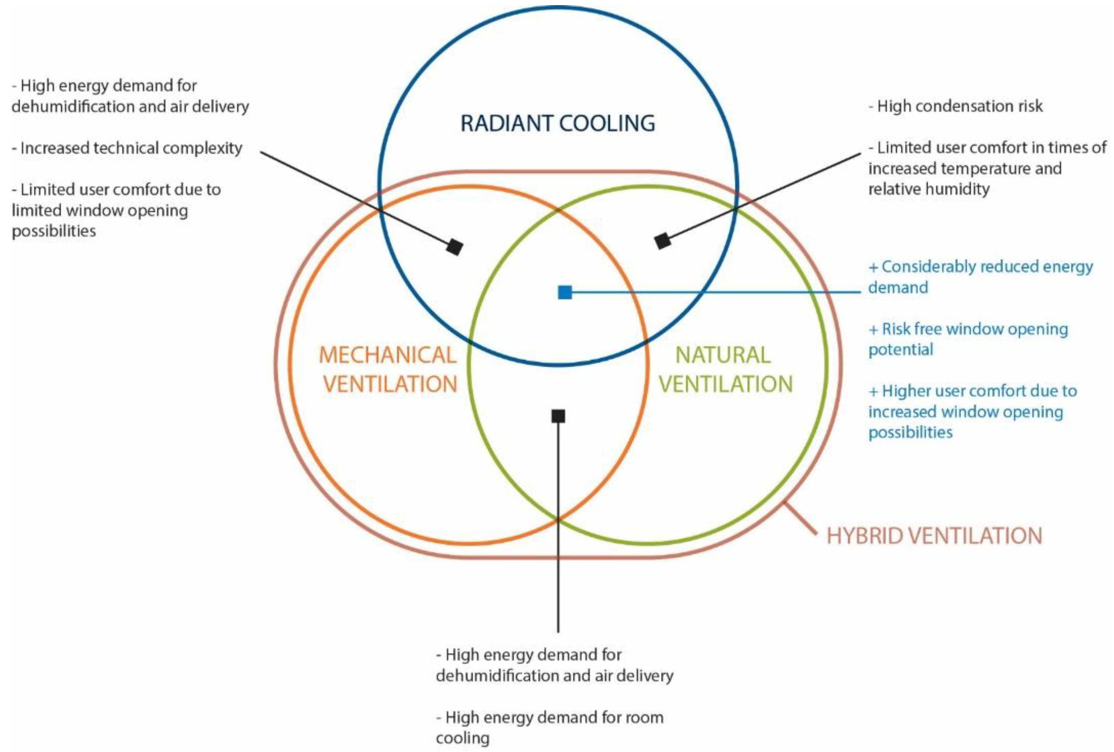
Figure 2.
Wide-angle interior view of the studio-classroom.

Figure 3.
Elements of the cooling and hybrid ventilation concept.

Figure 4.
(Top) reflected ceiling plan of the classroom, showing the radiant cooling panels integrated into the false ceiling. (Bottom) isometric of the simulation model showing the windows and the wall integrated panels.
Figure 4.
(Top) reflected ceiling plan of the classroom, showing the radiant cooling panels integrated into the false ceiling. (Bottom) isometric of the simulation model showing the windows and the wall integrated panels.

Figure 5.
Seasonal average daily air temperature (Ta; in red), dew point temperature (Td; in purple) (both on the primary axis) and relative humidity (Rh; in blue, on the secondary axis).
Figure 5.
Seasonal average daily air temperature (Ta; in red), dew point temperature (Td; in purple) (both on the primary axis) and relative humidity (Rh; in blue, on the secondary axis).

Figure 6.
Overview of the control strategies.

Figure 7.
Determination of Tsup using the point–slope form of straight-line equations.

Figure 8.
Air supply temperature with respect to outdoor temperature in Case (6).
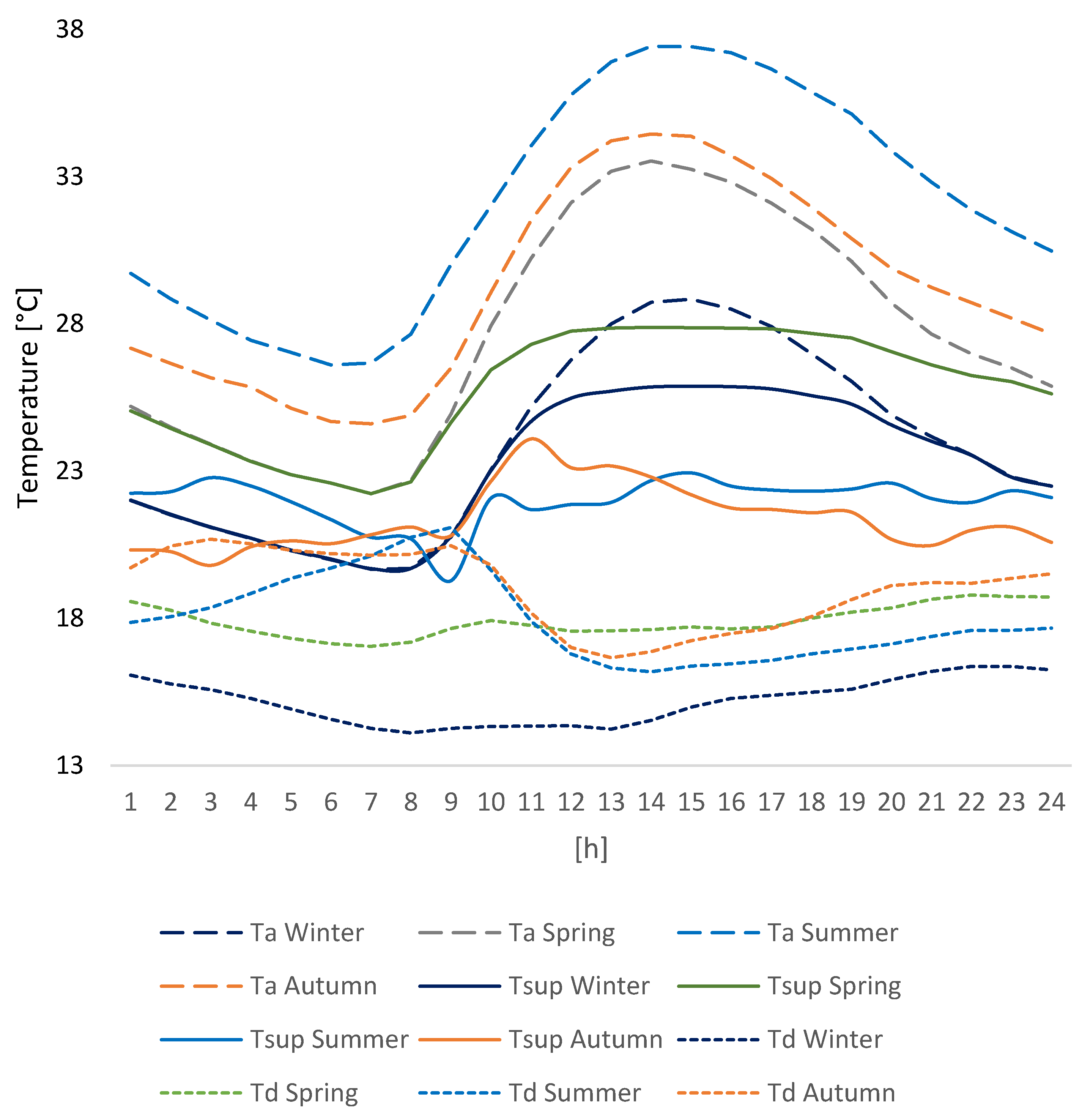
Figure 9.
Seasonal daily average cooling load against Tdif for Case (2).

Figure 10.
Average daily total hours of risk-free window opening potential. (Primary axis: The columns represent the duration of openings in each season with respect to the operation strategy, Secondary axis: the corresponding daily cooling energy demand is depicted in red dots).
Figure 10.
Average daily total hours of risk-free window opening potential. (Primary axis: The columns represent the duration of openings in each season with respect to the operation strategy, Secondary axis: the corresponding daily cooling energy demand is depicted in red dots).

Figure 11.
Comparison of Tdif against Tsup for selected cases.
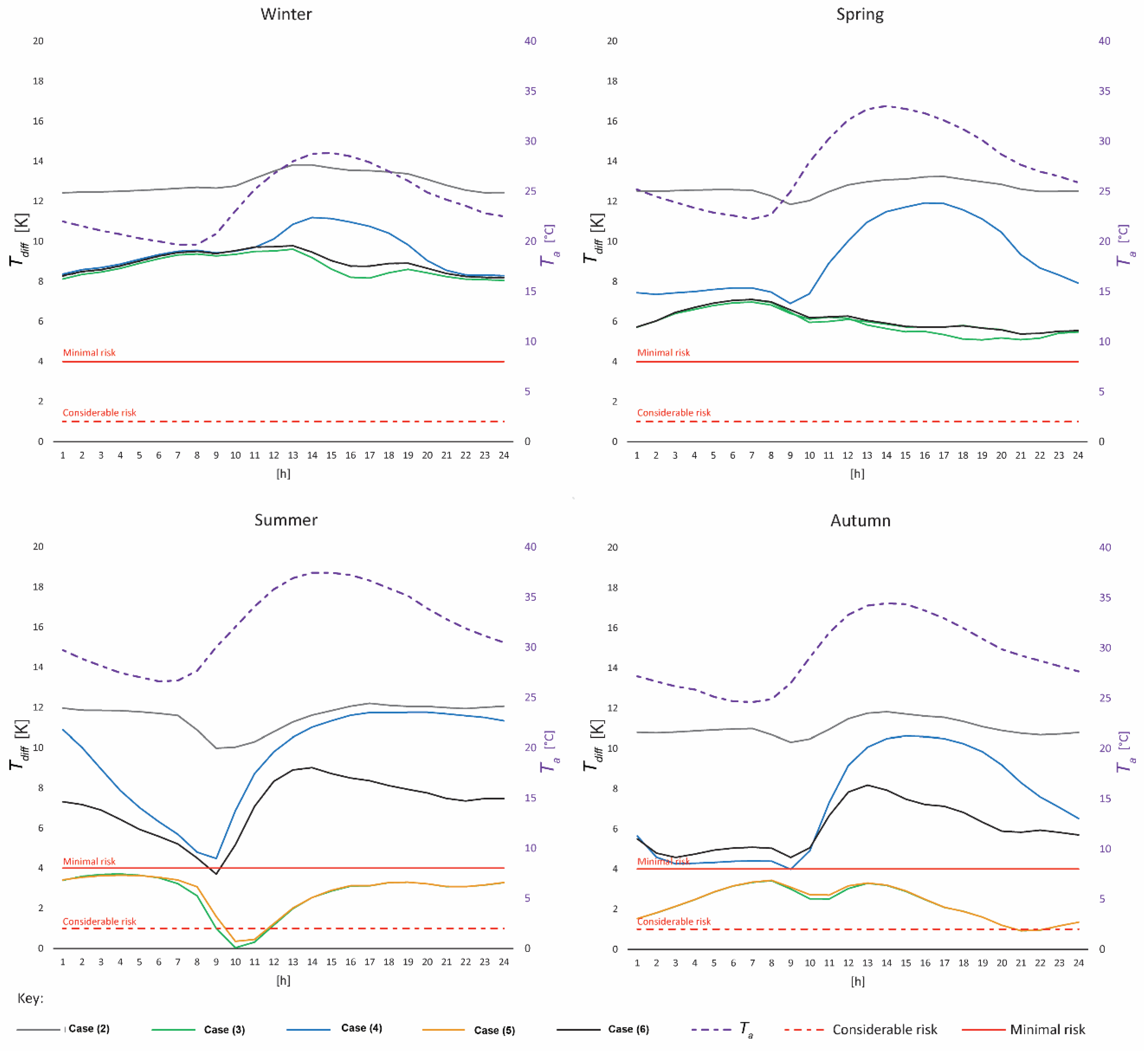
Figure 12.
Comparison of presented best strategies against the reference case (Case (2)).

Figure 13.
Results of the CFD simulation for Case (6) at 09:00 AM, in summer.
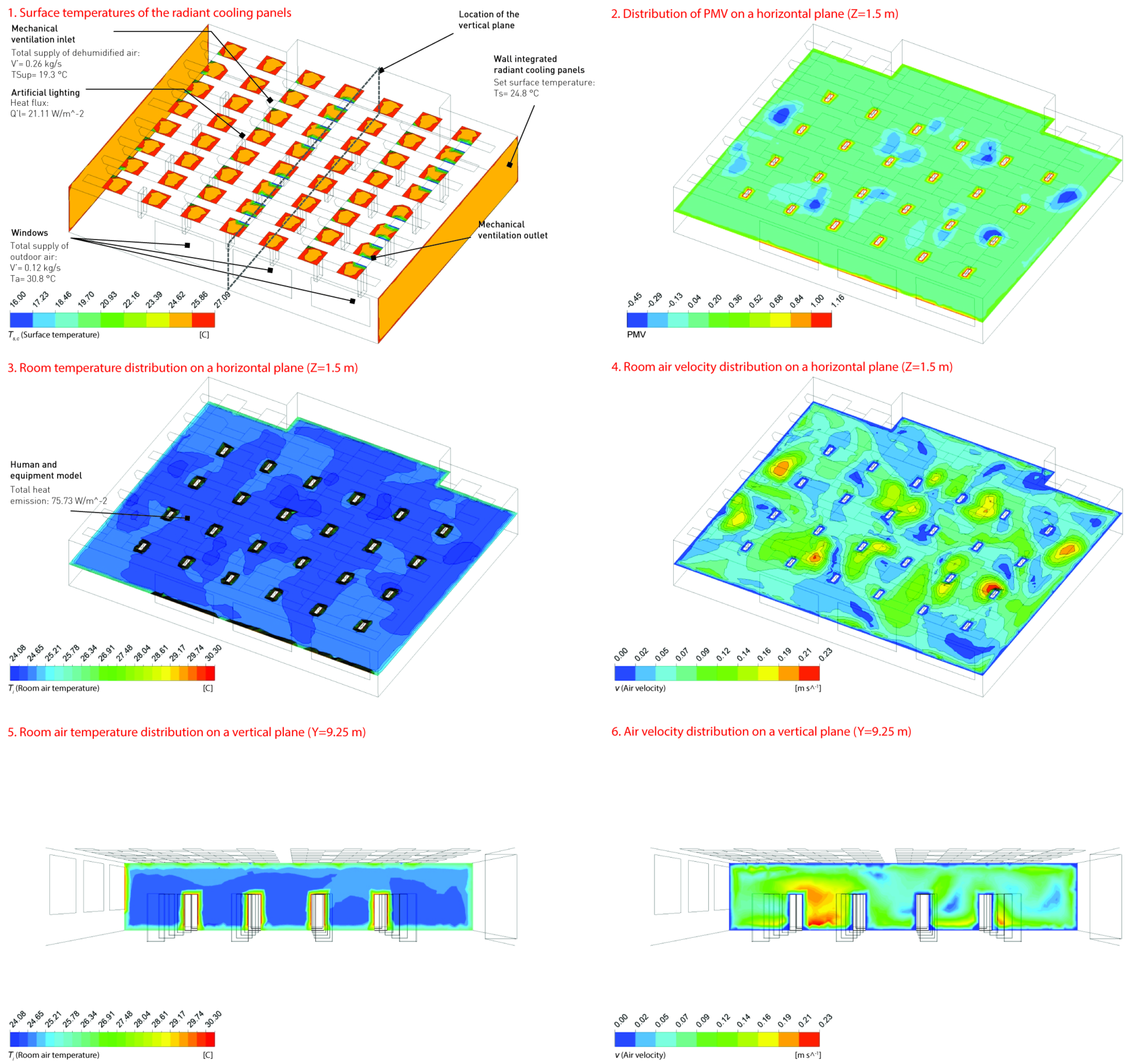
Figure 14.
Results of the CFD simulation for Case (6) at 09:00 AM in autumn.
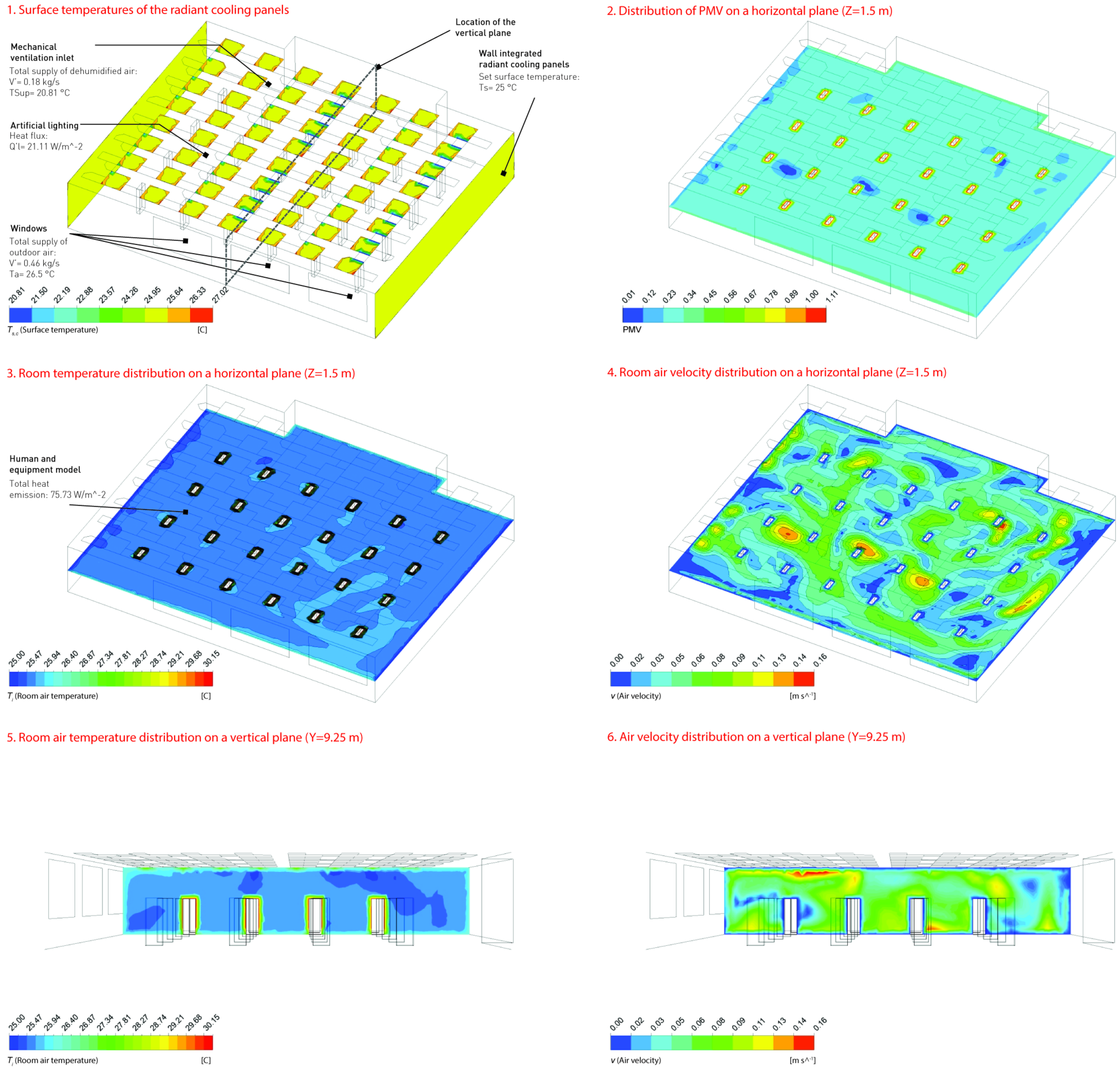
Figure 15.
Hx-diagram illustrating the simulated hybrid ventilation conditions.


Table 1.
Simulation cases and the related control strategies; AA: All-air, AW: Air–Water, H: Hybrid ventilation, Ti: Room temperature.
Table 1.
Simulation cases and the related control strategies; AA: All-air, AW: Air–Water, H: Hybrid ventilation, Ti: Room temperature.
| Façade | Unit | Case (1) | Case (2) | Case (3) | Case (4) | Case (5) | Case (6) |
|---|---|---|---|---|---|---|---|
| Window fraction | (%) | 40 | 40 | 40 | 40 | 40 | 40 |
| Frame fraction | (%) | 28 | 10 | 10 | 10 | 10 | 10 |
| Solar heat gain coefficient (gglass) | (%) | 30 | 59 | 59 | 59 | 59 | 59 |
| Light transmittance (tglass) | (%) | 43 | 72 | 72 | 72 | 72 | 72 |
| Rate of heat transfer (Ug) | (W/m2·K) | 1.6 | 1.2 | 1.2 | 1.2 | 1.2 | 1.2 |
| Window opening grade (WOG) | (%) | - | - | 50 | 50 | 50 | 50 |
| Window opening threshold (WOT) | (°C) | - | - | 28 | 26 | 28 | 28 |
| Cooling and MV | |||||||
| Control strategy of Tsup | (°C) | 16 °C | 16 °C | STR_1 | STR_2 | STR_3 | STR_4 |
| Room set temperature (Tset, rm) | (°C:°C) | 18–19 | 21–26 | 21–26 | 21–26 | 21–26 | 21–26 |
| Air supply control strategy | (-) | Ti + CO2 | CO2 | CO2 | CO2 | CO2 | CO2 |
| Cooling system | (-) | AA | AW | H | H | H | H |
Table 2.
Meshing parameters and the set values.
| Parameter | Unit | Value |
|---|---|---|
| Relevance center | (-) | Fine |
| Initial size seed | (-) | Active assembly |
| Smoothing | (-) | High |
| Transition | (-) | Slow |
| Span angle center | (-) | Fine |
| Minimum edge length | (m) | 0.0150 |
| Maximum face size | (m) | 0.3708 |
| Maximum cell size | (m) | 0.7406 |
| Growth rate | (m) | 1.2000 |
Table 3.
Framework of the conducted computational fluid dynamics (CFD) simulations.
| Season | Natural Ventilation | Mechanical Ventilation | Radiant Cooling | Room | |||||||
|---|---|---|---|---|---|---|---|---|---|---|---|
| Ta | V′w | m′w | Rh | Tsup | V′m | m′m | Q′c | Q′c | Ts,c | Ti | |
| [-] | [°C] | [m3/h] | [kg/s] | [%] | [°C] | [m3/h] | [kg/s] | [W/m2] | [kW] | [°C] | [°C] |
| Summer | 30.02 | 244.20 | 0.08 | 76.00 | 16.00 | 1011.00 | 0.33 | 24.24 | 16.00 | 24.79 | 25.80 |
| Autumn | 26.50 | 1443.28 | 0.47 | 75.75 | 20.81 | 542.50 | 0.18 | 49.03 | 6.10 | 25.05 | 25.45 |
Table 4.
Maximum risk-free window opening frequency.
| Season | Best Strategy | WOT | RF-WOPot | Cooling Demand |
|---|---|---|---|---|
| (-) | (°C) | (h/davg.) | (kWh/davg.) | |
| Winter | STR_1 | 26 | 24 | 45 |
| Spring | STR_1 | 28 | 24 | 111 |
| Summer | STR_2 | 26 | 9 | 46 |
| Autumn | STR_4 | 28 | 18 | 209 |
Table 5.
Calculation of mixed air condition and the potential risk of condensation.
| Variable | Unit | Summer | Autumn |
|---|---|---|---|
| Tsup | (°C) | 16.00 | 20.81 |
| m1 | (kg/h) | 1204.2 | 642.6 |
| Ta | (°C) | 30.02 | 26.50 |
| m2 | (kg/h) | 288 | 1688.76 |
| Rh | (%) | 76.00 | 75.75 |
| L1,2 | (mm) | 13.50 | 0 |
| L1 | (mm) | 2.61 | 0 |
| L2 | (mm) | 10.89 | 0 |
| Ts,c | (°C) | 24.79 | 25.05 |
| Td | (°C) | 20.30 | 20.81 |
| Tdif | (°C) | 4.49 | 4.24 |
| Ti | (°C) | 25.80 | 25.67 |
| v | (m/s) | 0.14 | 0.14 |
| MRT | (°C) | 27.15 | 25.54 |
© 2018 by the author. Licensee MDPI, Basel, Switzerland. This article is an open access article distributed under the terms and conditions of the Creative Commons Attribution (CC BY) license (http://creativecommons.org/licenses/by/4.0/).
Share and Cite
MDPI and ACS Style
Bayoumi, M. Method to Integrate Radiant Cooling with Hybrid Ventilation to Improve Energy Efficiency and Avoid Condensation in Hot, Humid Environments. Buildings 2018, 8, 69. https://doi.org/10.3390/buildings8050069
AMA Style
Bayoumi M. Method to Integrate Radiant Cooling with Hybrid Ventilation to Improve Energy Efficiency and Avoid Condensation in Hot, Humid Environments. Buildings. 2018; 8(5):69. https://doi.org/10.3390/buildings8050069
Chicago/Turabian StyleBayoumi, Mohannad. 2018. "Method to Integrate Radiant Cooling with Hybrid Ventilation to Improve Energy Efficiency and Avoid Condensation in Hot, Humid Environments" Buildings 8, no. 5: 69. https://doi.org/10.3390/buildings8050069
Note that from the first issue of 2016, this journal uses article numbers instead of page numbers. See further details here.