Optimization of Replaced Grinding Wheel Diameter for Surface Grinding Based on a Cost Analysis

Abstract

Based on a cost analysis, a method of identifying and predicting optimum replaced grinding wheel diameter (D_e.op) in a surface grinding operation for 9CrSi steel material was developed in this study. The D_e.op value was determined by minimizing the cost function. An experimental design was set up, and a computational program was developed to perform the experiment in order to calculate the D_e.op value. Furthermore, the impact of the grinding process parameters such as the initial grinding wheel diameter, the grinding wheel width, the total dressing depth, the Rockwell hardness of the workpiece, the radial grinding wheel wear per dress, and the wheel life on the D_e.op value were investigated. Moreover, the impacts of the cost components such as the machine tool hourly rate and the grinding wheel cost on the D_e.op value were given. Based on that, a mathematical model was proposed to determine the D_e.op value. The predicted D_e.op value was also verified by an experiment. The obtained result shows that the difference between the experimental D_e.op value and the predicted D_e.op value is within 1.7%, indicating that the mathematical model proposed in the study is reliable.

1. Introduction

Grinding is an operation applied in almost every type of manufacturing process. The grinding process is extensively used during finishing operations for discrete components [1,2]. When requiring precise tolerances and smooth surfaces for the final machining of components, grinding is expected to be an effective processing method. However, the grinding process is a costly procedure [3]. In industries, it can account for about 20–25% of the expenditure on machining operations [3]. Thus, this process should be used at optimal conditions.

Previous research works have studied the problem of optimizing technology parameters in order to enhance quality and productivity in grinding processes. For instance, Peters and Aerens [4] analyzed process parameters to minimize the total grinding time in an external cylindrical grinding process without intermediate dressing. Since then, this field has been continuously advanced by more constraints [5]. The relevance to the optimization of grinding and dressing parameters has been proposed for maximizing the material removal rate [3], minimizing the grinding time [6], as well as minimizing the dressing and grinding costs [7]. These works have implemented optimization problems with different grinding methods such as external cylindrical grinding [4,8,9], surface grinding [10,11,12,13,14,15], and internal grinding [16]. These optimization problems have addressed not only traditional grinding machines [3,4,5,6,7,8,9,10,11,12,13,14,15,16] but also CNC milling machines [17]. They have established different objective functions. For instance, in a recent study [9], Pi et al. presented a cost optimization method for internal cylindrical grinding operations. In this work, based on the calculation of the D_e.op value, the grinding cost is significantly reduced. Regarding surface grinding in recent years, several research works have focused on optimizing surface grinding process parameters [10] in order to obtain a high accuracy of the surface finishing process through the analysis of grinding parameters [11,12,13]. A proposed methodology was presented for computing optimal machining parameters in order to achieve a high production rate and good surface quality of machine components [14]. Recently, an experimental study for surface grinding was proposed in [15]. In this study, the D_e.op value is determined from the experiment.

This paper is concerned with the optimization of the replaced grinding wheel diameter in a surface grinding operation for 9CrSi steel material based on the formulation of the manufacturing cost per piece. This work was continuously developed by the proposed formula [9], which has not been extended to surface grinding and has not yet been employed to carefully evaluate grinding process parameters and cost components. Therefore, in this paper, the D_e.op value is determined by minimizing the cost function. Moreover, the grinding technology parameters, such as the initial grinding wheel diameter, the total dressing depth, the radial grinding wheel wear per dress, and the wheel life are given to evaluate the effects of these parameters on the optimal exchange grinding wheel diameter. Additionally, the influence of the cost components on the D_e.op value is also considered. To identify the effect of these parameters, an experiment is built, and a computational program is also established to carry out the experiment. The research results will help manufacturers solve the problem of selecting conditions for initial technological parameters since they allow manufacturers to determine and set up optimal parameters of pre-machining grinding conditions to increase the economic and technical effectiveness of the grinding process.

2. Methodology

In this section, the cost analysis of the surface grinding process is investigated. Based on the findings, the relationship between the cost of the surface grinding process and the replaced grinding wheel diameter is studied. In addition, the relationship between the replaced grinding wheel diameter and the technological parameters in the grinding process is analyzed. This is the theoretical basis on which we determine the D_e.op value to minimize the cost of the surface grinding process. For the surface grinding process, the grinding cost per part can be computed as follows:

$$C_{\mathrm{part}}=t_s{C}_{mh}+C_g$$

(1)

where:

• t_s is the manufacturing time (h) which will be discussed in more detail following;
• C_mh is the machine tool hourly rate (USD/h) including wages, cost of maintenance etc.;
• C_g is the grinding wheel cost per workpiece (USD/workpiece). C_g can be expressed as follows:

$$C_g=C_{g,p}/n_{p,w}$$

(2)

where C_g,p is the grinding wheel cost per piece (USD/piece) and n_p,w is the total number of workpieces ground by a grinding wheel. n_p,w can be determined as follows [18]:

$$n_{p,w}=(D_0-D_e)n_{p,d}/[2(W_{pd}+a_{ed})]$$

(3)

where $D_0$ is the initial grinding wheel diameter (mm); $D_e$ is the replaced grinding wheel diameter (mm); W_pd is the radial grinding wheel wear per dress (mm/dress); $a_{ed}$ is the total depth of dressing cut (mm); n_p,d is the number of workpieces per dress. n_p,d can be determined as follows:

$$n_{p,d}=T_w/t_c$$

(4)

where $T_w$ is the longevity of the grinding wheel (h) and $t_c$ is the grinding time (h). In surface grinding, the grinding time can be determined as follows:

$$t_c=l_c{w}_c{a}_{e,tot}/(1000v_w{v}_f{f}_d{N}_t).$$

(5)

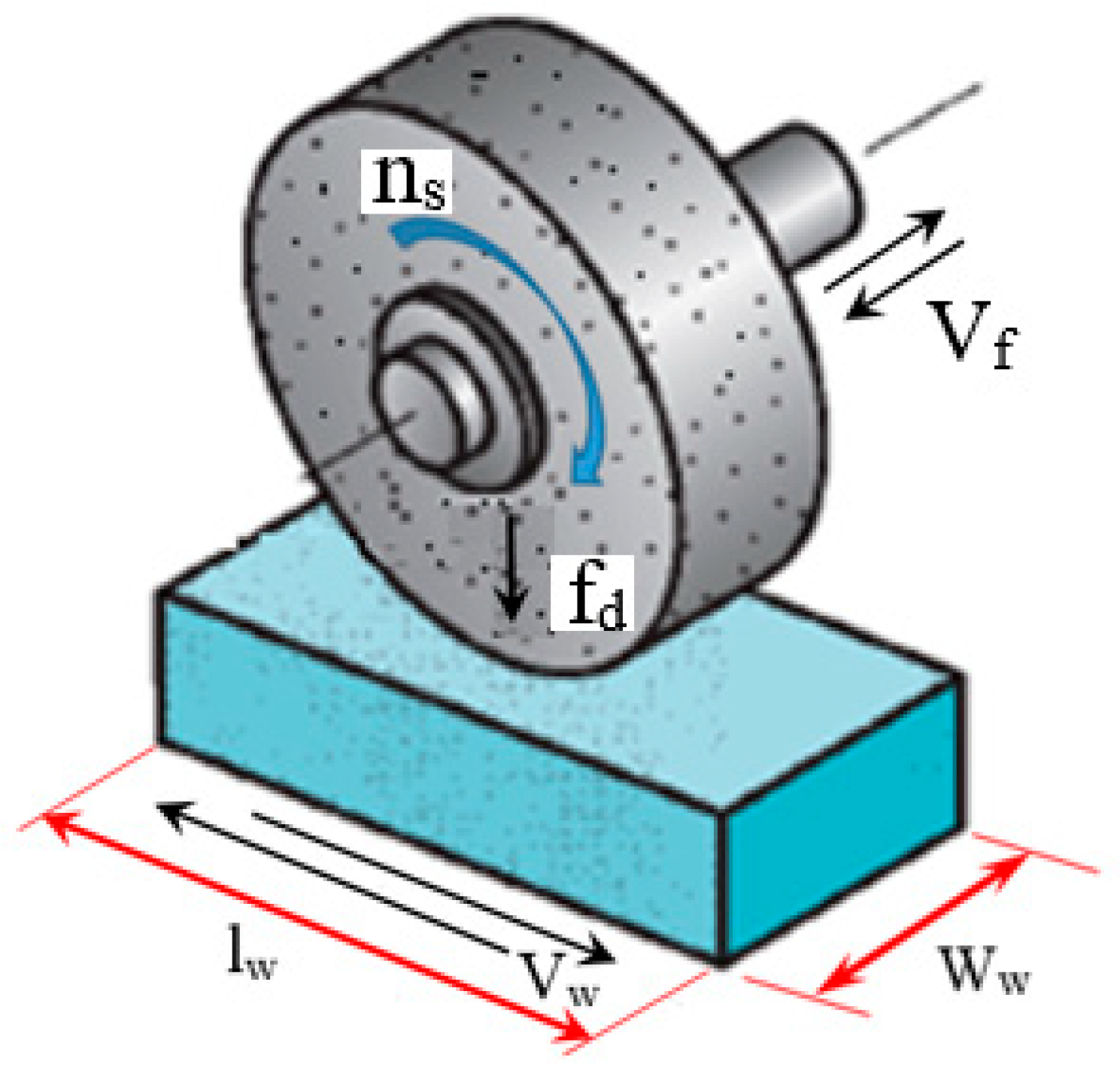
In Equation (5), $l_c$ is the calculated grinding length (mm); $l_c=l_w+\left(20\dots 30\right)$ where $l_w$ is the length of the workpieces (mm); $w_c$ is the calculated grinding width (mm); $w_c=w_w+w_{gw}+5$, where $w_w$ is the width of the workpieces (mm) (see Figure 1) and $w_{gw}$ is the grinding wheel width (mm); $a_{e,tot}$ is the total depth of cut (mm); $v_w$ is the speed of the workbench (m/s); $v_f$ is the work feed rate (mm/min); $f_d$ is the downfeed (mm/pass) (see Figure 1); $N_t$ is the number of workpieces per grinding time.

To determine t_c by Equation (5), several parameters, $v_w, v_f$, and $f_d$, are determined as follows. With grinding carbon steel, alloy steel, and brass, the work speed $v_w$ can be computed from the data in [15], which depends on the Rockwell hardness of workpiece HRC. Thus, $v_w$ can be written as the following regression equation:

$$v_w=0.0598HR{C}^{1.4}.$$

(6)

Based on the required roughness grade number $N_{Ra}$ and the grinding wheel width $w_{gw}$, the work feed rate $v_f$ can be computed from the following regression equation [18]:

$$v_f=46w_{gw}^{0.983}/N_{Ra}^{2.44}.$$

(7)

The downfeed $f_d$ can be calculated as follows [18]:

$$f_d=f_{d,t}{c}_1{c}_2{c}_3$$

(8)

where $f_{d,t}$ is the tabulated downfeed (mm/pass). When grinding tool steel, the tabulated downfeed $f_{d,t}$ can be determined as follows [18]:

$$f_{d,t}=0.649a_{e,tot}^{0.651}{v}_f^{-0.985}$$

(9)

where $a_{e,tot}$ is the total depth of cut and $v_f$ is the work feed rate.

In Equation (8), $c_1, c_2$, and $c_3$ are coefficients; $c_1$ depends on the workpiece material and required tolerance grade $tg$. When grinding tool steel, $c_1$ can be calculated as follows [15]:

$$c_1=0.61t{g}^{0.466}.$$

(10)

The coefficient $c_2$ is determined as follows [15]:

$$c_2=0.0292d_s^{0.5151}/D_w^{0.4949}$$

(11)

where $d_s$ is the grinding wheel diameter and $D_w$ is the density of the workpiece loaded on the machine table. The value of the coefficient $c_3$ depends on the grinding machine age; $c_3=1$ if the age is less than 10 years, $c_3=0.85$ if the age ranges from 10 to 20 years, and $c_3=0.7$ if the age is more than 20 years [15].

In Equation (1), $t_s\left(h\right)$ can be identified as follows:

$$t_s=t_c+t_{lu}+t_{sp}+t_{d,p}+t_{cw,p}.$$

(12)

Here, $t_c, t_{lu}, t_{sp}, t_{d,p}$, and $t_{cw,p}$ are the grinding time (as shown in Equation (5)), the time for loading and unloading workpiece, the spark-out time, the dressing time per piece, and the time for changing a grinding wheel per workpiece, respectively. $t_{sp}, t_{d,p}$, and $t_{cw,p}$ can be expressed as follows:

$$t_{sp}=l_c{\mathrm{w}}_c/(1000v_{\mathrm{w}}{v}_f{N}_t),$$

(13)

$$t_{d,p}=t_d/n_{p,d},$$

(14)

$$t_{cw,p}=t_{cw}/n_{p,w}.$$

(15)

Substituting Equation (3) into Equation (15), $t_{cw,p}$ can be written as follows:

$$t_{cw,p}=2t_{c\mathrm{w}}(w_{pd}+a_{ed}\left)\right[n_{p,d}(D_0-D_e)].$$

(16)

Based on the formulation of the above manufacturing cost per piece, it is indicated that the replaced grinding wheel diameter (D_e) affects the cost of the surface grinding process. For a certain technological condition where $D_0=500 \mathrm{mm}$; $W_{gw}=40 \mathrm{mm}$; $z=0.1 \mathrm{mm};$ $C_{mh}=10 \mathrm{USD}/\mathrm{h};C_{gw}=30 \mathrm{USD}/\mathrm{piece};n_s=1450 \mathrm{rpm}$; $n_{pd}=35$; $a_{ed}=0.1 \mathrm{mm}$; $T_w=20 \min$; $W_{pd}=0.02 \mathrm{mm}/\mathrm{dress}$, the relationship between the grinding cost and the D_e value (calculated by Equation (1)) is built as shown in Figure 2. It is observed that the D_e value strongly affects the cost of grinding operations. When the D_e value increases from 200 to 475 mm, the grinding cost decreases from 0.0014 to 0.001 USD/part. However, as the D_e value increases from 475 to 500 mm, the grinding cost grows rapidly from 0.001 to 0.0016 USD/part. In particular, the grinding cost is minimum when the D_e value equals an optimum value of $D_{e,op}=475 \mathrm{mm}$, which is much larger than the conventional D_e value (in this case about 200 to 250 mm).

From the above analyses, the $D_{e,op}$ value can be determined by minimizing the grinding cost per piece $C_{part}$. Thus, the cost function of the surface grinding process can be expressed as follows:

$$\min C_{\sin }=f(D_e)$$

(17)

with the constraint as:

$$D_{e,min}\le D_e\le D_{e,max}.$$

(18)

Besides, the D_e,op value depends on various technology factors. From the cost analysis of the surface grinding process, it is revealed that there are eight main factors affecting the D_e,op value. The eight main factors include the initial grinding wheel diameter D₀, the grinding wheel width W_gw, the total depth of dressing cut a_ed, the Rockwell hardness of the workpiece HRC, the wheel life T_w, the radial grinding wheel wear per dress W_pd, the machine tool hourly rate C_mh, and the grinding wheel cost C_gw. Therefore, the function of the optimum replaced grinding wheel diameter can be presented as follows:

$$D_{e,op}=f(D_0,W_{gw},a_{ed},HRC,T_w,W_{pd},C_{mh},C_{gw}).$$

(19)

3. Experimental Work

In this section, the eight abovementioned factors are selected to evaluate their effects on the D_e,op value. Simultaneously, an experimental design with a two-level factorial design with a half fraction was set up. The values of these input factors in experimental tests are presented in

Table 1. Grinding parameters for the experiment.

Factor	Code	Unit	Low	High
Initial grinding wheel diameter	$D_0$	mm	250	500
Grinding wheel width	Wgw	mm	20	50
Total depth of dressing cut	$a_{ed}$	mm	0.1	0.2
Rockwell hardness of workpiece	HRC	-	20	65
Wheel life	$T_w$	min	10	30
Radial grinding wheel wear per dress	$W_{pd}$	mm	0.01	0.03
Machine tool hourly rate	$C_{mh}$	USD/h	5	15
Grinding wheel cost	$C_{gw}$	USD/part	15	50

.

Accordingly, 128 $=2^{\left(8-1\right)}$ experiments were conducted. In addition, based on the equations in Section 2, a computational program was established to determine the D_e,op value in each experiment. Various levels of the input parameters and the output response are shown in

Table 2. Experimental plans and output response.

Std Order	Run Order	CenterPt	Blocks	${\mathit{D}}_{\mathbf{0}}$	Wgw	${\mathit{a}}_{\mathit{e}\mathit{d}}$	HRC	${\mathit{T}}_{\mathit{w}}$	${\mathit{W}}_{\mathit{p}\mathit{d}}$	${\mathit{C}}_{\mathit{m}\mathit{h}}$	${\mathit{C}}_{\mathit{g}\mathit{w}}$	${\mathit{D}}_{\mathit{e},\mathit{o}\mathit{p}}$
97	1	1	1	250	20	0.1	20	10	0.03	15	15	231.75
82	2	1	1	500	20	0.1	20	30	0.01	15	50	474.52
51	3	1	1	250	50	0.1	20	30	0.03	5	50	220.16
89	4	1	1	250	20	0.1	65	30	0.01	15	50	232.38
108	5	1	1	500	50	0.1	65	10	0.03	15	50	459.16
104	6	1	1	500	50	0.2	20	10	0.03	15	50	447.25
…
54	127	1	1	500	20	0.2	20	30	0.03	5	15	465.51
9	128	1	1	250	20	0.1	65	10	0.01	5	50	210.3

. The obtained results of the conducted experiments would be the basis to analyze the influences of these parameters on the D_e,op value.

Grinding experiments were performed on a surface grinder (MGK7120 × 6, Moto–Yokohama, made in Japan) by using a Vietnamese grinding wheel with a JIS code of Cn80MV1 300 × 127 × 30, as shown in Figure 3. The 9CrSi steel plates with dimensions of 100 mm × 80 mm × 30 mm were used as the work material. The specifications of the grinding conditions and grinding wheels are shown in

Table 3. Specifications of grinding conditions.

Machine and Equipment	Specifications
Grinding machine	Surface grinder of Moto–Yokohama (made in Japan)
Grinding wheel	Cn46MV1 300 × 127 × 30 (made in Vietnam)
Workpiece material	90CrSi
Workpiece dimensions	100 × 60 × 30 mm3
Cooling modes	Caltex Aquatex 3180
Environment	Flood
Dresser	Multi diamond dresser, 3908-0088C type 2 (made in Russia)

.

4. Results and Discussions

Based on the data reported in Table 2, the influence of the factors on the D_e,op value was determined as shown in Figure 4. It can be clearly seen that D₀ value has the largest effect on the D_e,op value (the left side in Figure 3). For the other parameters such as a_ed, T_w, W_ed, C_mh, and C_gw, the effect of these parameters on the D_e,op value is much smaller than that of the D₀ factor. In addition, the D_e,op value is not affected by the W_gw and HRC parameters.

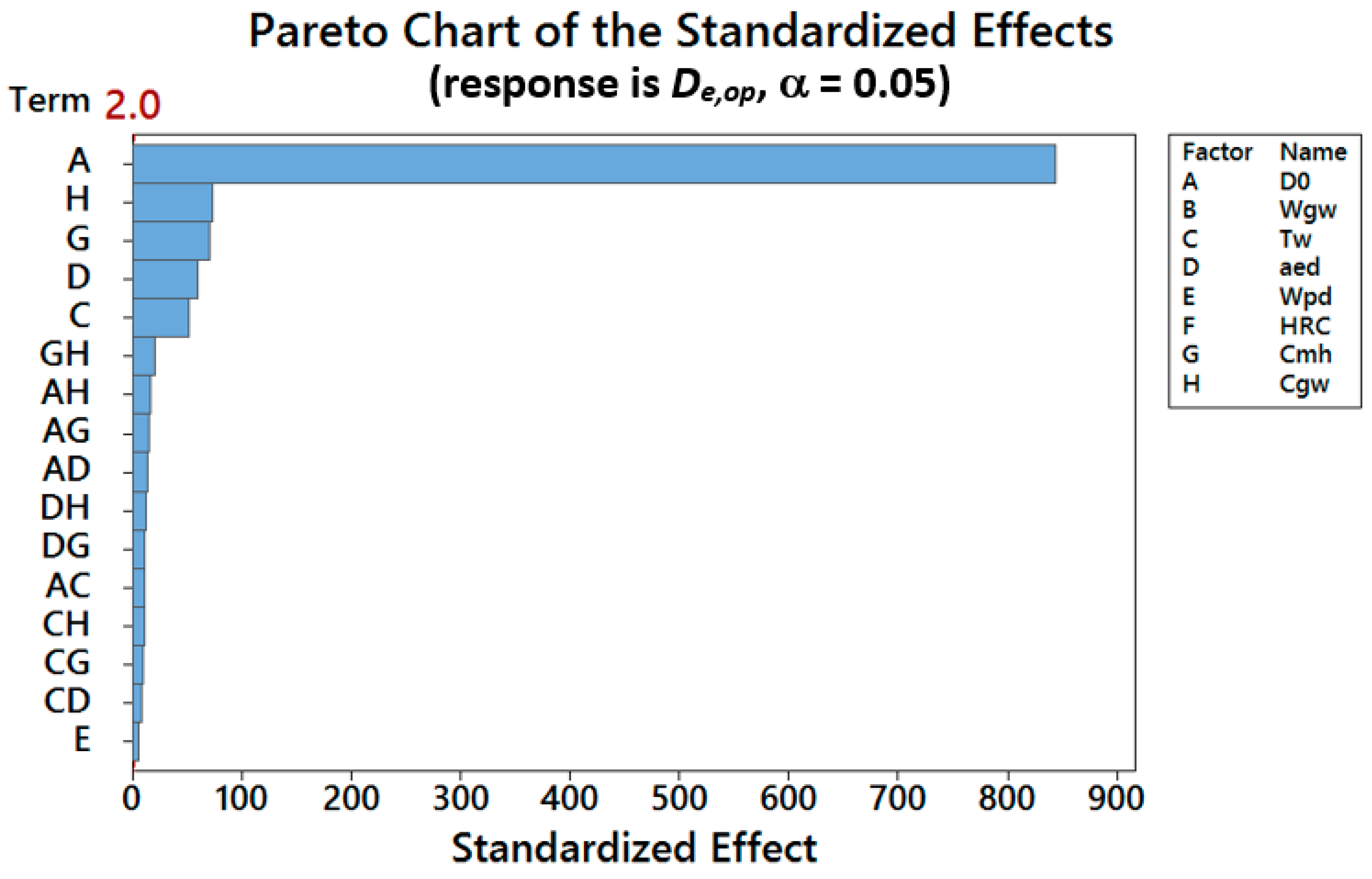
The influence of the factors can be seen more clearly in Figure 5, which shows the Pareto chart of the standardized effects for determining the magnitude and the importance of the influence on the D_e,op value. For the response model, the parameters are statistically significant at the 0.05 level. As presented in this figure, the magnitude of the influence on the grinding process parameters is arranged from the lowest value to the highest value. The largest influence on the optimum diameter belongs to the initial grinding wheel D₀ (factor A in Figure 5). The influence is gradually reduced in the sequence of several grinding process parameters, such as the grinding wheel cost C_g (factor H in Figure 5), the machine tool hourly rate C_mh (factor G in Figure 5), the wheel life T_w (factor E in Figure 5), and the total depth of dressing cut a_ed (factor C in Figure 5). The factor with the smallest effect is the radial grinding wheel wear per dress W_pd (factor F in Figure 5). Significantly, as noted above, the optimum exchanged diameter is not affected by the grinding wheel width W_gw (factor B in Figure 5) and the Rockwell hardness of the workpiece HRC (factor D in Figure 5).

However, the Pareto chart (as shown in Figure 5) merely displays the magnitude of the effects. Thus, the normal plot of the standardized effects was established as shown in Figure 6 to evaluate the effects of increasing or decreasing the response. The distribution of the standardized effects to most of the factors is close to the reference line (red line in Figure 6). The positive effects of the 10 factors including D₀, T_w, C_mh and the interactions AE, AG, GH, CG, CE, CF, EH increase the D_e,op value when these factors change from a low value to a high value. Meanwhile, the other parameters such as a_ed, Cg, W_pd and the interactions AH, EG, AC, CH have negative effects. When they alter from a low value to a high value, the D_e,op value declines. In addition, the initial grinding wheel diameter D₀ has the largest magnitude compared to other factors. Therefore, the optimum replaced grinding wheel diameter is tremendously influenced by the initial grinding wheel diameter D₀.

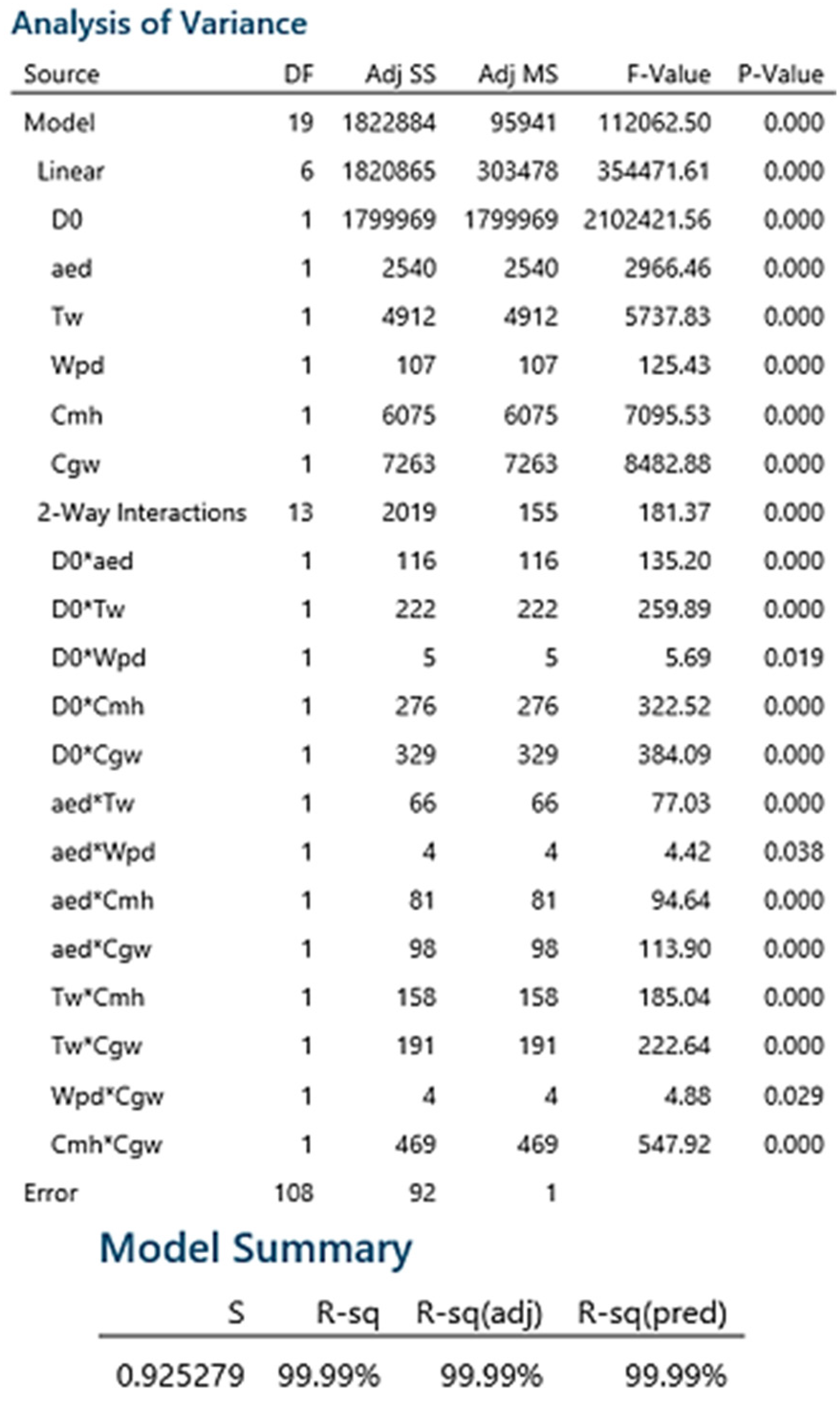
Figure 7 depicts the estimated effects and coefficients for the D_e,op value. It can be recognized that those parameters including D₀, a_ed, T_w, W_pd, C_mh, C_g and the interactions between D₀ and a_ed, D₀ and T_w, D₀ and C_mh, D₀ and C_gw, a_ed and T_w, a_ed and W_pd, a_ed and C_mh, a_ed and C_gw, T_w and C_gw, T_w and C_mh, W_pd and C_gw, C_mh and C_gw have significant effects on a response because their P-values are lower than 0.05. Remarkably, the D₀ factor has the largest effect on the D_e,op value in comparison with the other factors.

Consequently, after carrying out experiments and collecting results, the data were analyzed and processed by using Minitab 18 software. Based on that, the mathematical model, which shows the relationship between the D_e,op value and the significant effect parameters, is expressed as follows:

$$\begin{array}{l}{D}_{e,op}=-1.29+0.95384D_0-67.02a_{ed}+0.0045T_{\mathrm{w}}-51.1W_{pd}-0.2469C_{mh}-0.3436C_{gw}-\\ -0.1522D_0{a}_{ed}+0.001055D_0{T}_{\mathrm{w}}-0.156D_0{W}_{pd}+00235D_0{C}_{mh}-0.000733D_0{C}_{gw}+\\ +1.436a_{ed}{T}_w+344a_{ed}{W}_{pd}+3.183a_{ed}{C}_{mh}-0.9975a_{ed}{C}_{\mathrm{gw}}-0.02225T_w{C}_{mh}+\\ +0.006973T_w{C}_{gw}-1.032W_{pd}{C}_{gw}+0.021879C_{mh}{C}_{gw}\end{array}$$

(20)

In order to evaluate the appropriateness of the formula (20), the D_e,op value computed by Equation (20) was compared with the experimental result found in [15]. The values of the factors used for the optimum diameter calculation in Equation (20) and for the experimental design were the same, i.e., D₀ = 300 mm; a_ed = 0.115 mm; T_w = 22.5 min; W_pd = 0.02 mm/dress; C_mh = 5 USD/h; C_g = 25 USD/piece. Accordingly, the D_e,op value was 266.86 mm according to Equation (20) and was 265 mm as determined by the experiment. The difference between the formulation and the experiment can be expressed as follows:

$${\mathsf{\delta }}_{D_{op}}=\frac{(269.59-265)\times 100}{269.59}\%=1.7\%,$$

(21)

The results from Equation (21) show that the D_e,op value is calculated by the Equation (20) in accordance with the optimum value obtained from the experiment. Thus, the proposed method can be used to determine the D_e,op value in surface grinding operations for 9CrSi steel material.

5. Conclusions

This study developed a method to minimize the grinding cost based on determining the D_e,op value in surface grinding operations for 9CrSi steel material. A mathematical model for determining the D_e,op value was proposed. In addition, the influence of eight factors including D₀, W_gw, a_ed, HRC, T_w, W_pd, C_mh, and C_g on the D_e,op value in the surface grinding process was determined by designing and conducting a simulation experiment. From the experimental results of the study, some findings can be presented:

(1)

The initial grinding wheel diameter D₀ has the largest effect on the D_e,op value. Meanwhile, the grinding wheel width (W_gw) and the Rockwell hardness of workpiece (HRC) do not affect the D_e,op value.

(2)

Three factors including D₀, T_w, C_mh have positive influences on the D_e,op value. Meanwhile, the other parameters such as a_ed, C_gw, W_pd have negative influences on the D_e,op value.

(3)

For a certain set of technological parameters, i.e., $D_0=300\mathrm{mm};a_{ed}=0.115\mathrm{mm};T_w=22.5\min ;W_{pd}=0.02\mathrm{mm}/\mathrm{dress};C_{mh}=5\mathrm{USD}/\mathrm{h};C_g=25\mathrm{USD}/\mathrm{piece}$, the D_e,op value is 266.86 mm. After carrying out an experiment with those values of the input parameters, the obtained result shows that the difference between the experimental D_e.op value and the prediction D_e.op value is 1.7%, indicating that the model proposed in this study is reliable.