A Comparative Study on Arrhenius and Johnson–Cook Constitutive Models for High-Temperature Deformation of Ti₂AlNb-Based Alloys

Abstract

In order to thoroughly understand the quantitative relationships between the flow stress and deformation conditions for Ti₂AlNb-based alloys at elevated temperatures, the Arrhenius and Johnson–Cook constitutive models are analyzed and identified on the basis of the uniaxial tensile tests. The Johnson–Cook model is modified so that the referenced temperature range can be randomly adjusted. By experimental verification, the Arrhenius model (including the Backofen model) is suitable for the deformation at relatively low strain-rate deformation, such as the superplastic forming, and the modified J–C model is applicable for the deformation within a wide range of strain rates. For deformation at high temperatures, the constitutive model enables a more precise description of the effect of strain on the flow stress through introducing as train-softening factor exp(sε).

1. Introduction

In recent years, various constitutive models have been developed to describe the flow behaviors of metals and alloys. According to the construction processes and principles, the constitutive models are mainly classified into two categories: phenomenological and physics-based constitutive models [1,2,3]. For various materials, it is required to use different constitutive models to describe the deformation behaviors due to the differences in their mechanical properties. For the same material, different constitutive models can be also used due to the dependence of its mechanical properties on the deformation conditions such as temperatures and strain rates. Commonly used constitutive models for deformation at elevated temperature are the Arrhenius model, the Johnson–Cook (J–C) model, and so forth.

For the Arrhenius model [2,4], the effects of temperature and strain rate on the flow behavior are considered, expressed as:

$$\dot{\epsilon }=A{\left[\sinh \left(\alpha \sigma \right)\right]}^{n^{\prime }}\exp \left[-Q/\left(RT\right)\right]$$

(1)

where $\dot{\epsilon }$ is the strain rate (s⁻¹), both A and α are material constants, σ is the flow stress (MPa), n’ is the stress exponent, Q is the deformation activation energy (J·mol⁻¹), R is the ideal gas constant, and T is the deformation temperature (K).

The hyperbolic sine function sinh(x) is described with Taylor series expansion as:

$$\sinh \left(x\right)=\left(e^x-e^{-x}\right)/2=x+\frac{x^3}{3!}+\frac{x^5}{5!}+\frac{x^7}{7!}+\dots$$

(2)

When x is small, the above terms that are more than third power have very small values that can be ignored, then, sinh(x) ≈ x. In contrast, if x is large, the value of item e^−x can be ignored, leading to sinh(x) ≈ e^x/2 and sinh(ασ) ≈ e^ασ/2.

Through the above analysis, the Arrhenius equation can be simplified as:

$$\{\begin{array}{ll}\dot{\epsilon }=A_1{\sigma }^{n^{\prime }}\exp \left[-Q/\left(RT\right)\right]& \mathrm{when}\alpha \sigma \mathrm{smaller}\\ \dot{\epsilon }=A_2\exp \left(\alpha n^{\prime }\sigma \right)\exp \left[-Q/\left(RT\right)\right]& \mathrm{when}\alpha \sigma \mathrm{larger}\\ \dot{\epsilon }=A{\left[\sinh \left(\alpha \sigma \right)\right]}^{n^{\prime }}\exp \left[-Q/\left(RT\right)\right]& \mathrm{when}\alpha \sigma \mathrm{taking}\mathrm{any}\mathrm{value}\end{array}$$

(3)

where A₁ = Aα^n’, A₂ = A/2^n’. Generally, the first formula is utilized for creep deformation with low stress, the second formula is applied for rapid deformation at lower temperatures, and the third formula is suitable for wider temperatures and strain rates ranges [1].

For the first formula, the equation can be modified to Equation (4) when the deformation temperature T is a constant, as given below:

$$\dot{\epsilon }=A_1{\sigma }^{n^{\prime }}\mathrm{or}\sigma =\frac{1}{A_1}{\dot{\epsilon }}^{\frac{1}{n^{\prime }}}=K{\dot{\epsilon }}^m$$

(4)

where K is the material constant, m is the strain rate sensitivity exponent. This equation is also called the Norton or Backofen constitutive equation [5,6,7].

However, the Arrhenius and Norton or Backofen equations do not consider the effect of strain on the flow stress, therefore, they are only suitable for the deformation without strain-hardening effect.

For materials exhibiting both the strain and strain-rate hardening, the plastic deformation obeys:

$$\sigma =K{\epsilon }^n{\dot{\epsilon }}^m$$

(5)

which is also called the Rosserd equation [8,9].

Similarly, if the effects of strain, strain rate, and temperature are all taken into account, Equation (5) can be expressed as:

$$\sigma =K{\epsilon }^n{\dot{\epsilon }}^m\exp [Q/(RT)]$$

(6)

which is known as the classical Norton–Hoff constitutive model [10].

If considering the second form of Equation (3) available for rapid dynamic deformations, the stress is obtained as a function of strain rate logarithm. Considering the strain-rate sensitivity form, Johnson and Cook put forward the Johnson–Cook model in 1983 [11], which is used for high-temperature deformation of metals or alloys. The J–C model is in a simple format and is widely used in engineering [12,13,14]. Most numerical simulation software programs, such as LS-DYNA, MSC. Dytran, and ABAQUS/explicit, use the J–C model to simulate some dynamic processes. The effects of temperature, strain rate, and strain on the flow stress during deformation are all considered. The equation is shown as follows:

$$\sigma =\left(A+B{\epsilon }^n\right)\left(1+C\ln \dot{\epsilon }*\right)\left(1-T{*}^{m^{\prime }}\right)$$

(7)

where A is the yield strength (MPa), B is the exponential coefficient (MPa), C is the strain-rate-sensitive coefficient, m’ is the temperature-sensitive coefficient, $\epsilon$ is the true strain, n is the strain-hardening exponent, $\dot{\epsilon }*$ is the dimensionless strain rate, and $\dot{\epsilon }*$ can be expressed as:

$$\dot{\epsilon }*=\dot{\epsilon }/{\dot{\epsilon }}_0$$

(8)

where ${\dot{\epsilon }}_0$ is the reference strain rate (s⁻¹).

The relative temperature $T*$ is expressed as below:

$$T*=\left(T-T_r\right)/\left(T_m-T_r\right)$$

(9)

where $T_r$ is the room temperature (K), usually $T_r$ = 298 K, $T_m$ is the material melting temperature (K).

For the J–C model in Equation (7), the three brackets on the right represent strain hardening, strain-rate hardening, and temperature-softening effects of the material, respectively. The parameters A, B, n, C, and m’ always vary with the deformation conditions.

Titanium aluminides with compositions based around the stoichiometry Ti₂AlNb have received great attention as potential high-temperature structural materials [15,16]. In order to thoroughly understand the quantitative relationships between the flow stress and deformation conditions, including temperature, strain rate, and strain, the present work makes a comparative study using the Arrhenius and Johnson–Cook models to describe the high-temperature deformation behaviors. The prediction accuracy of each model under different deformation conditions is also evaluated and discussed.

2. Materials and Methods

The as-received material was a hot-rolled alloy sheet with a thickness of 1.3 ± 0.5 mm and a nominal composition of Ti-22Al-25Nb (at.%). The sheet was annealed for 2 h at 1000 °C after the final step of hot rolling at 940 °C. Uniaxial tensile tests were performed on an Instron 5500R machine (Instron Corp., Norwood, MA, USA) to investigate the deformation behavior of the alloy. The uniaxial testing set-up was mounted in a high-temperature furnace. The tensile specimens were prepared along the rolling direction, with a gage length of 10 mm and a width of 3 mm. To minimize the oxidation, the gage section of each specimen was coated with glass slurry. For each test, the specimen was heated to the set temperature and soaked for 5 min, and then was uniaxially stretched. To consider the effects of temperature and strain rate on the flow behavior, the tests were performed at initial strain rates ranging from 2.5 × 10⁻⁴ s⁻¹ to 8 × 10⁻³ s⁻¹ changing two times and temperatures ranging from 930 °C to 990 °C with an interval of 20 °C.

3. Results and Discussion

3.1. True Stress–Strain Curves

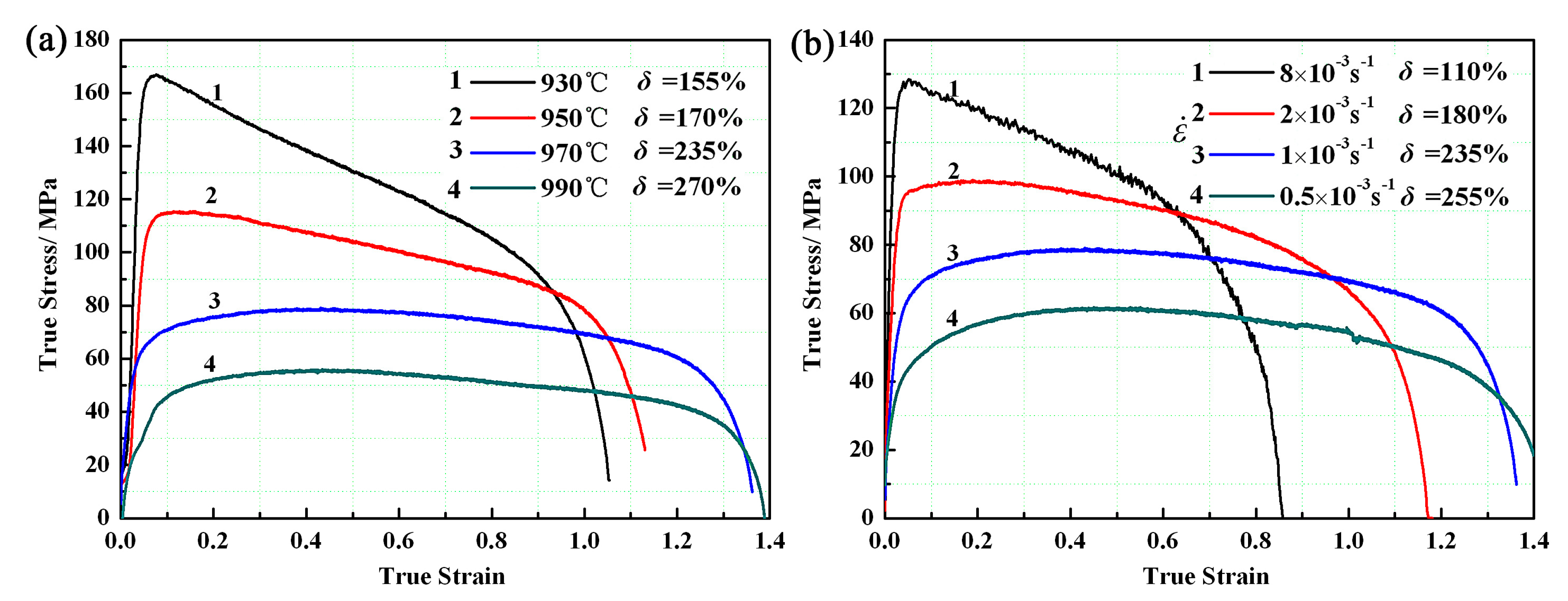
Figure 1 shows the true stress–strain curves of the alloy deformed at temperatures ranging between 930 °C and 990 °C, and strain rates ranging from 2.5 × 10⁻⁴ s⁻¹ to 8 × 10⁻³ s⁻¹.

The whole flow process in each curve can be divided into four stages: elastic, hardening, softening, and necking stages. In the elastic stage, the flow stress rose quickly. In the hardening stage, the flow stress became larger with the proceeding of deformation. The softening stage was characterized by the uniform and stable decreasing of flow stress. In the necking stage, the slope of curves increased and the flow stress dropped drastically. Obviously, the flow stress of the alloy is strongly dependent on the deformation conditions, including the deformation temperature, strain rate and strain. Therefore, the constitutive models should take all these influence factors into account. The uniform elongation δ increases with increasing temperature and decreasing strain rate, which is over 200% at the condition of T ≥ 970 °C and $\dot{\epsilon }\le 1\times {10}^{-3}{\mathrm{s}}^{-1}$, showing a superplasticity characteristic.

3.2. Arrhenius Model

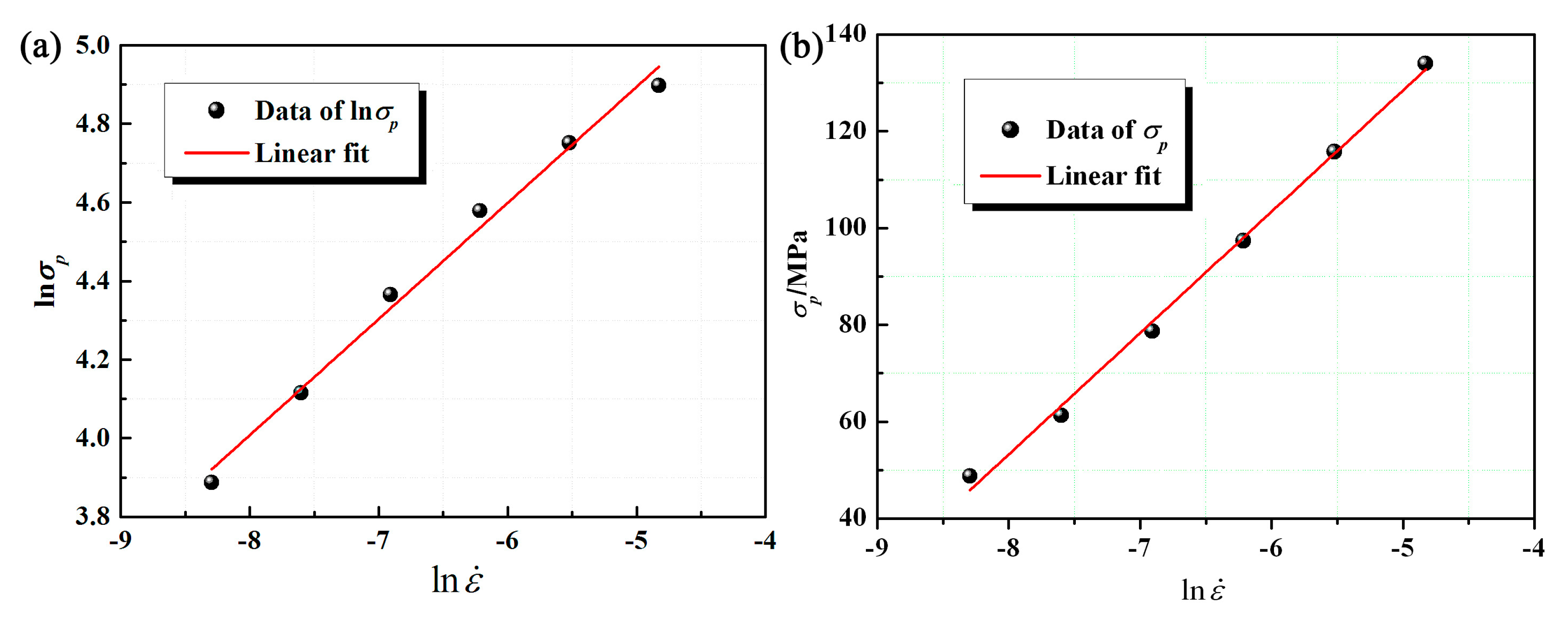
In the Arrhenius model shown in Equation (1), for a certain temperature, the values of A, Q, R, and T are constants. In order to evaluate the material parameters individually, sequential linear regressions are used to solve the parameters. The values of n’ and α can be determined by the following formulas:

$$n\prime =\frac{\partial \ln \dot{\epsilon }}{\partial \ln \sigma }$$

(10)

$$\alpha =\frac{1}{n\prime }\cdot \frac{\partial \ln \dot{\epsilon }}{\partial \sigma }$$

(11)

where σ is the peak value σ_p, the values of n’ and n’α are obtained by linear fitting between $\ln {\sigma }_p–\ln \dot{\epsilon }$ and ${\sigma }_p–\ln \dot{\epsilon }$, as shown in Figure 2. The fitted values of n(1/m) and α were equal to 3.383 and 0.0118, respectively. The values of ασ varied from 0.58 to 1.58 with strain rates varying from 2.5 × 10⁻⁴ s⁻¹ to 8 × 10⁻³ s⁻¹ at 970 °C, indicating a moderate stress level. Therefore, it is reasonable to choose the third formula of Equation (3) as the constitutive model.

When the temperature changes, the values of A, α, R, and n’ are constants while the value of Q varies with the temperature. The values of Q and A are calculated as follows:

$$Q=R\cdot n\prime \cdot \frac{d\left\{\ln \left[\sinh \left(\alpha \sigma \right)\right]\right\}}{d\left(1/T\right)}$$

(12)

$$A=\dot{\epsilon }\cdot {[\sinh (\alpha \sigma )]}^{-n\prime }\cdot \exp [Q/(RT)]$$

(13)

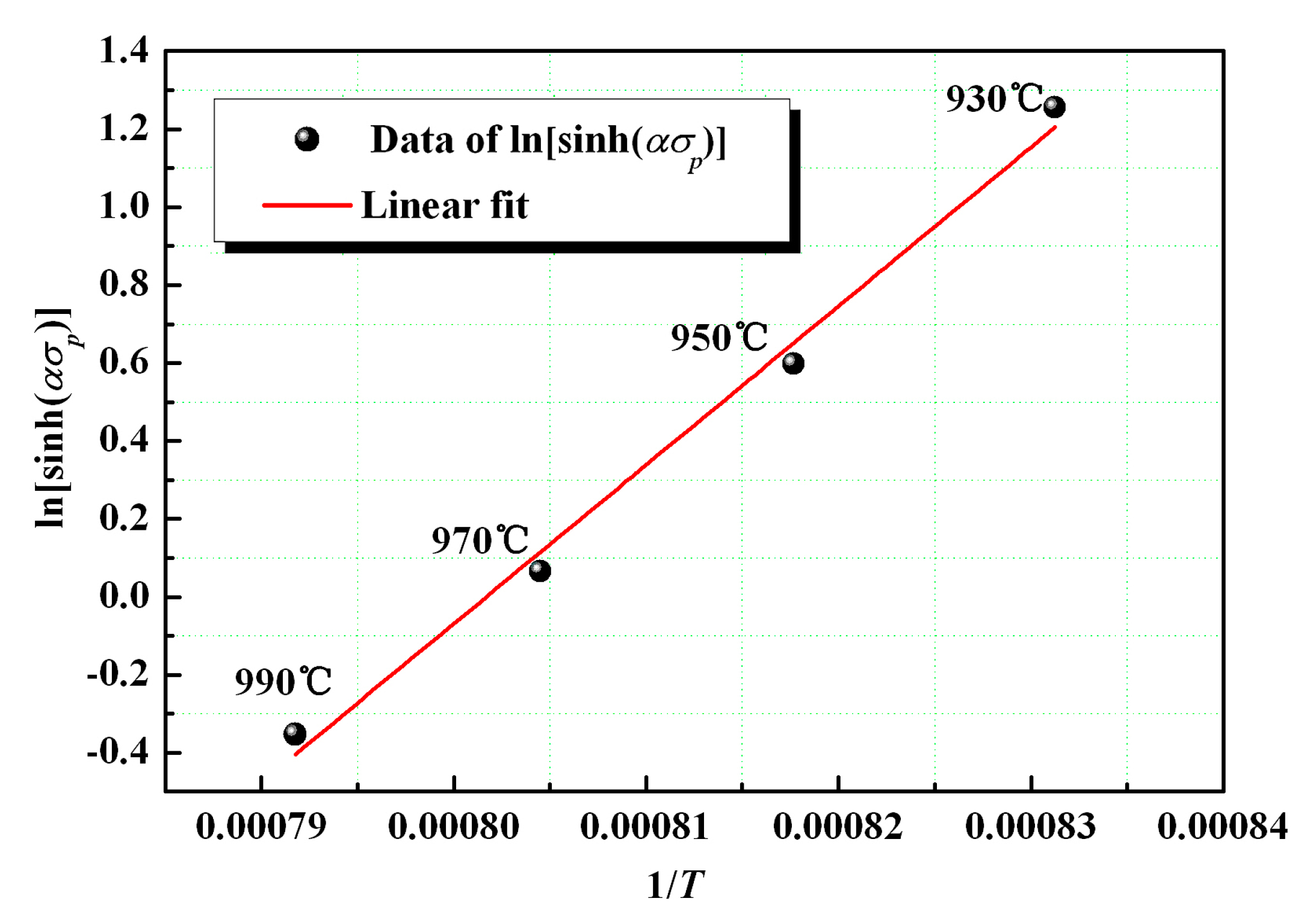
Substituting α and n’ values into Equation (12), the ln[sinh(ασ_p)] versus 1/T scatter can be plotted under a deformation strain rate of $1.0\times {10}^{-3}{\mathrm{s}}^{-1}$, as shown in Figure 3.

By the linear fitting, the value of $Q/(R\cdot n\prime )$ is equal to the slope of the plot and the values of Q (1146 kJ·mol⁻¹) and A (1.175 × 10⁴⁵) are finally obtained. Hence, the Arrhenius constitutive equation of the Ti-22Al-25Nb alloy sheet can be described as:

$$\dot{\epsilon }=1.175\times {10}^{45}\cdot {[\sinh (0.0118\sigma )]}^{3.383}\exp [-137846.59/T]$$

(14)

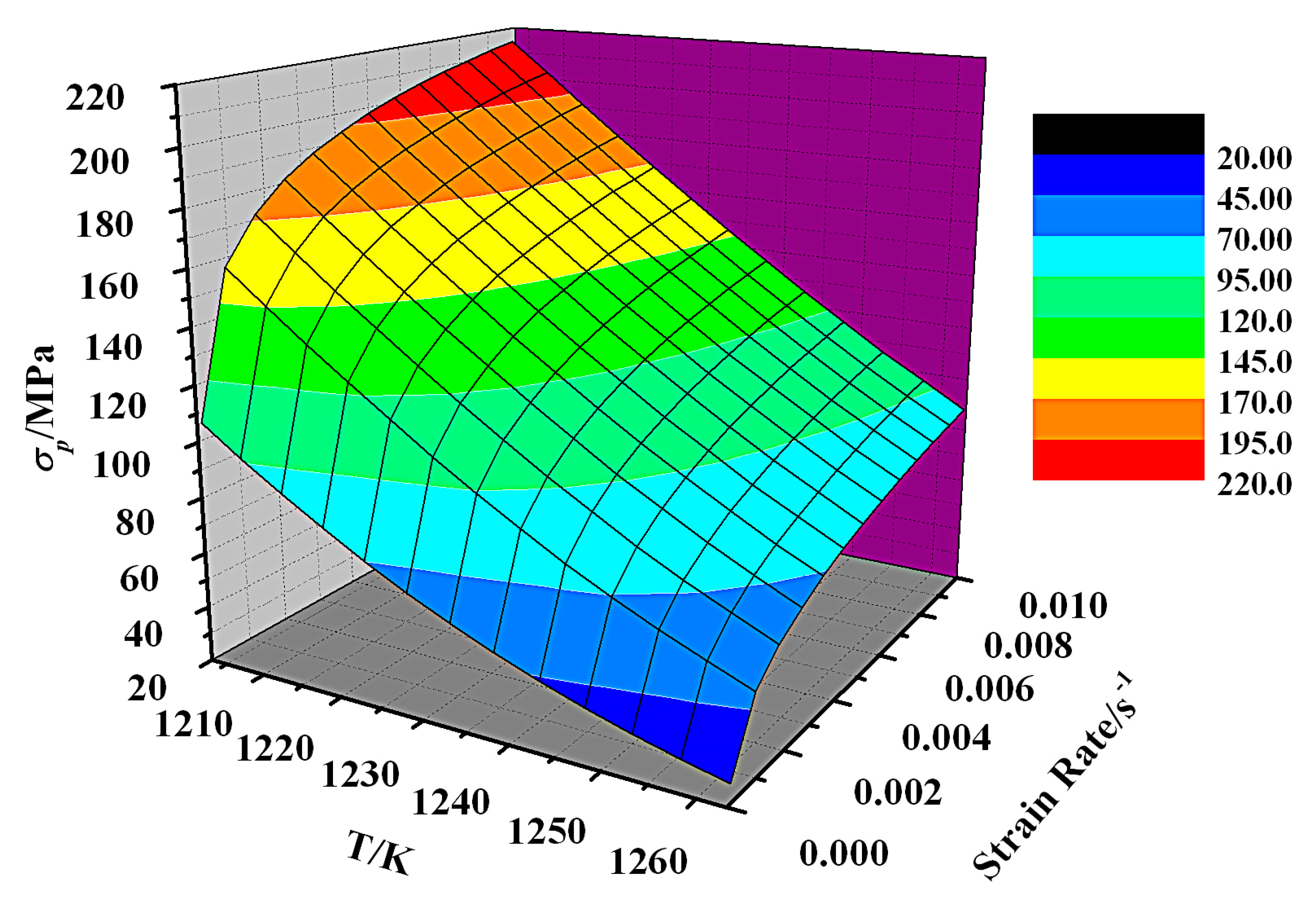
Since σ is a binary function of $\dot{\epsilon }$ and T with a curved surface graphically, as indicated in Figure 4, the peak stress of σ_p can be obtained from any point ($\dot{\epsilon }$, T).

As shown in Figure 1, the flow stress first achieved the peak and then decreased immediately, indicating that the alloy undergoes softening rather than hardening with increasing strain. However, when the deformation temperature is too high or the strain rate is too low, such as at T ≥ 970 °C and $\dot{\epsilon }\le 1\times {10}^{-3}{\mathrm{s}}^{-1}$, the strain softening effect is no more prominent and the flow stress can be maintained at a constant level for a larger strain, even exhibiting a superplasticity. In this case, the deformation behavior can be described by the Backofen equation.

Equation (15) can be obtained by taking natural logarithms on both sides of the Backofen model in Equation (4):

$$\ln \sigma =\ln K+m\ln \dot{\epsilon }$$

(15)

The strain rate sensitivity index m is the slope of $\ln \sigma -\ln \dot{\epsilon }$ curves. Under the deformation condition of T = 970 °C and $\dot{\epsilon }=2.5\times {10}^{-4}~8\times {10}^{-3}$, K and m were equal to 585.81 and 0.2956, respectively. Then, the Backofen constitutive equation was indicated as below:

$$\sigma =581.81{\dot{\epsilon }}^{0.2956}$$

(16)

With the further simultaneous consideration of strain, strain rate, and temperature effect on the flow stress, Equation (6) can be used. Taking natural logarithm on both sides, it can be described as follows:

$$\ln \sigma =\ln K+m\ln \dot{\epsilon }+Q/RT$$

(17)

The value of $\ln K+Q/RT$ is the intercept of $\ln \sigma –\ln \dot{\epsilon }$ curves (Figure 2a) and the determined value of K is 4.03 × 10⁻⁴⁶. Then, the Norton–Hoff constitutive equation with temperature variables is shown as below:

$$\sigma =4.03\times {10}^{-46}{\dot{\epsilon }}^{0.2956}\exp \left(137846.59/T\right)$$

(18)

For materials with both strain and strain-rate hardening, the deformation can be described using the Norton–Hoff equation (Equation (6)). As shown in Figure 1, the flow stress of Ti-22Al-25Nb alloy increased at the beginning and then decreased with straining, exhibiting both the hardening and softening effect. Since the strain softening is not considered in the Norton–Hoff equation, the model cannot be directly used for this alloy. In consideration of strain and thermal sensitivity based on Hensel–Spittel and Hirt laws [17], the modified Norton–Hoff equation is obtained by introducing a softening factor $\exp \left(bT+s\epsilon \right)$, as given in Equation (19):

$$\sigma =K{\epsilon }^n{\dot{\epsilon }}^m\exp \left(bT+s\epsilon \right)$$

(19)

where b is the temperature-softening coefficient and s is the strain-softening coefficient.

As known from the previous analysis, the hardening index n of the alloy at room temperature is equal to 0.11 and the strain-rate sensitivity index m is equal to 0.2956 at a temperature of 970 °C and strain rates ranging from 2.5 × 10⁻⁴ s⁻¹ to 8 × 10⁻³ s⁻¹.The parameters b and s are calculated in the following.

Taking natural logarithms on both sides of Equation (19):

$$\ln \sigma =\ln K+n\ln \epsilon +m\ln \dot{\epsilon }+bT+s\epsilon$$

(20)

Assuming the strain and strain rate are constants, the value of $\ln K+n\ln \epsilon +m\ln \dot{\epsilon }+s\epsilon$ is also a constant. The value of b is the slope of the $\ln \sigma -T$ curve shown in Figure 5, which is equal to −0.0184.

Assuming the temperature and strain rate are constants, the value of $\ln K+m\ln \dot{\epsilon }+bT$ is a constant. For a homogeneous deformation at a certain temperature and strain rate, Equations (21) and (22) can be obtained if $\epsilon ={\epsilon }_1$, $\sigma ={\sigma }_1$ and $\epsilon ={\epsilon }_2$, $\sigma ={\sigma }_2$:

$$\ln {\sigma }_1=\ln K+\mathrm{nln}{\epsilon }_1+m\ln \dot{\epsilon }+bT+c\dot{\epsilon }+s{\epsilon }_1$$

(21)

$$\ln {\sigma }_2=\ln K+\mathrm{nln}{\epsilon }_2+m\ln \dot{\epsilon }+bT+c\dot{\epsilon }+s{\epsilon }_2$$

(22)

Subtracting Equation (22) from Equation (21), the value of s can be calculated as follows:

$$s=\frac{\ln \frac{{\sigma }_1}{{\sigma }_2}-n\cdot \ln \frac{{\epsilon }_1}{{\epsilon }_2}}{{\epsilon }_1-{\epsilon }_2}$$

(23)

From the stress–strain curves, if ${\epsilon }_1=0.5$, ${\sigma }_1=78$ MPa and ${\epsilon }_2=1.0$, ${\sigma }_2=69.4$ MPa, the value of s obtained from Equation (23) is equal to −0.3861. When T = 970 °C and $\dot{\epsilon }=1.0\times {10}^{-3}{\mathrm{s}}^{-1}$, the peak stress is 78.7 MPa at a strain of 0.4. Substituting the peak stress ${\sigma }_p$ into Equation (19), the constant K is obtained as 6.71 × 10¹². Finally, the modified Norton–Hoff equation considering the softening factor $\exp \left(bT+s\epsilon \right)$ is obtained as follows:

$$\sigma =6.71\times {10}^{12}{\epsilon }^{0.11}{\dot{\epsilon }}^{0.2956}\exp \left(-0.0184T-0.3681\epsilon \right)$$

(24)

3.3. Johnson–Cook Model

For the Johnson–Cook model in Equation (7) and the definition of the relative temperature $T*$ in Equation (9), the model can be used from the room temperature to the melting temperature. However, the material parameters A, α, n, and m are all tested at room temperature. For the deformation at elevated temperature, on one hand, dynamic recovery or recrystallization may occur, resulting in the reduced or even disappeared strain-hardening effect. Therefore, it is unreasonable to use the parameters A, B, and n tested at room temperature. On the other hand, for most metals, the strain-rate sensitivity varies with temperature or strain rate at elevated temperatures. Therefore, the strain-rate sensitivity exponent m tested at room temperature is not accurate to study the elevated temperature deformation.

For the Ti-22Al-25Nb alloy in the present study, strong strain softening occurs within the temperature range of 930~990 °C, and the strain-rate sensitivity is greatly dependent on the deformation temperature and strain rate. Therefore, it is not reasonable to use the strict format of the model to describe the elevated temperature deformation. In fact, the initial Johnson–Cook model essentially takes the yield stress at room temperature and a certain strain rate as the referential flow stress and represents the effects of the strain, strain rate, and temperature increment on the referential flow stress (yield stress). Therefore, for elevated temperature deformation, when taking the flow stress in the specified condition range as the referential flow stress, it is feasible to study the flow behavior in the specified condition, such as at a certain temperature and a certain strain rate.

Equation (7) can be transformed:

$$1-\frac{\sigma }{\left(A+B{\epsilon }^n\right)\left(1+C\ln \dot{\epsilon }*\right)}=T{*}^m$$

(25)

When the strain rate takes the referential one, $\left(1+C\ln {\dot{\epsilon }}^{*}\right)$ = 1, the flow stress at room temperature ${\sigma }_r=A+B{\epsilon }^n$ and the flow stress at melting point σ_m = 0. The relations between the flow stress and temperature can be understood as:

$$\frac{{\sigma }_r-\sigma }{{\sigma }_r-{\sigma }_m}={\left(\frac{T_r-T}{T_r-T_m}\right)}^m$$

(26)

or

$$\sigma ={\sigma }_r-\left({\sigma }_r-{\sigma }_m\right)T{*}^m$$

(27)

It is obvious that the relative increment of stress varies with temperature in power function. When the strain rate varies, the Johnson–Cook model can be described as:

$$\sigma =\left[{\sigma }_r-\left({\sigma }_r-{\sigma }_m\right)T{*}^m\right]\left(1+C\ln \dot{\epsilon }*\right)$$

(28)

where the reference temperature is the room temperature T_r and the temperature range is [T_r, T_m]. In view of the format of Equation (28), if the temperature range is randomly selected as [T_l, T_h], where T_r represents the referential temperature, Equation (28) can be generalized as:

$$\begin{gathered} \sigma =\left[{\sigma }_l-\left({\sigma }_l-{\sigma }_h\right)T{*}^m\right]\left(1+C\ln \dot{\epsilon }*\right) \\ T*=\left(T-T_l\right)/\left(T_h-T_l\right) \end{gathered}$$

(29)

where ${\sigma }_l$ and ${\sigma }_h$ are the flow stress at T_l and T_h, respectively. In this case, the applicable temperature range of the constitutive model (Equation (29)) can be randomly selected. This model format is an improvement on the initial J–C model, whose validity will be verified through the following experimental results.

Here, taking the temperature T = 930 °C (1203 K) as the referential temperature and the strain rate ${\dot{\epsilon }}_0=1.0\times {10}^{-3}{\mathrm{s}}^{-1}$ as the referential strain rate, the J–C model of the Ti-22Al-25Nb alloy under the condition of T = 930~990 °C and $\dot{\epsilon }=2.5\times {10}^{-4} ~8\times {10}^{-3}{\mathrm{s}}^{-1}$ is established as below:

$$T*=\left(T-T_l\right)/\left(T_h-T_l\right)=\left(T-1203\right)/60$$

(30)

Taking natural logarithms on both sides of Equation (26) as below:

$$\ln \frac{{\sigma }_r-\sigma }{{\sigma }_r-{\sigma }_m}=m\ln \left(\frac{T_r-T}{T_r-T_m}\right)$$

(31)

Obviously, the value of m is the slope of Equation (31).

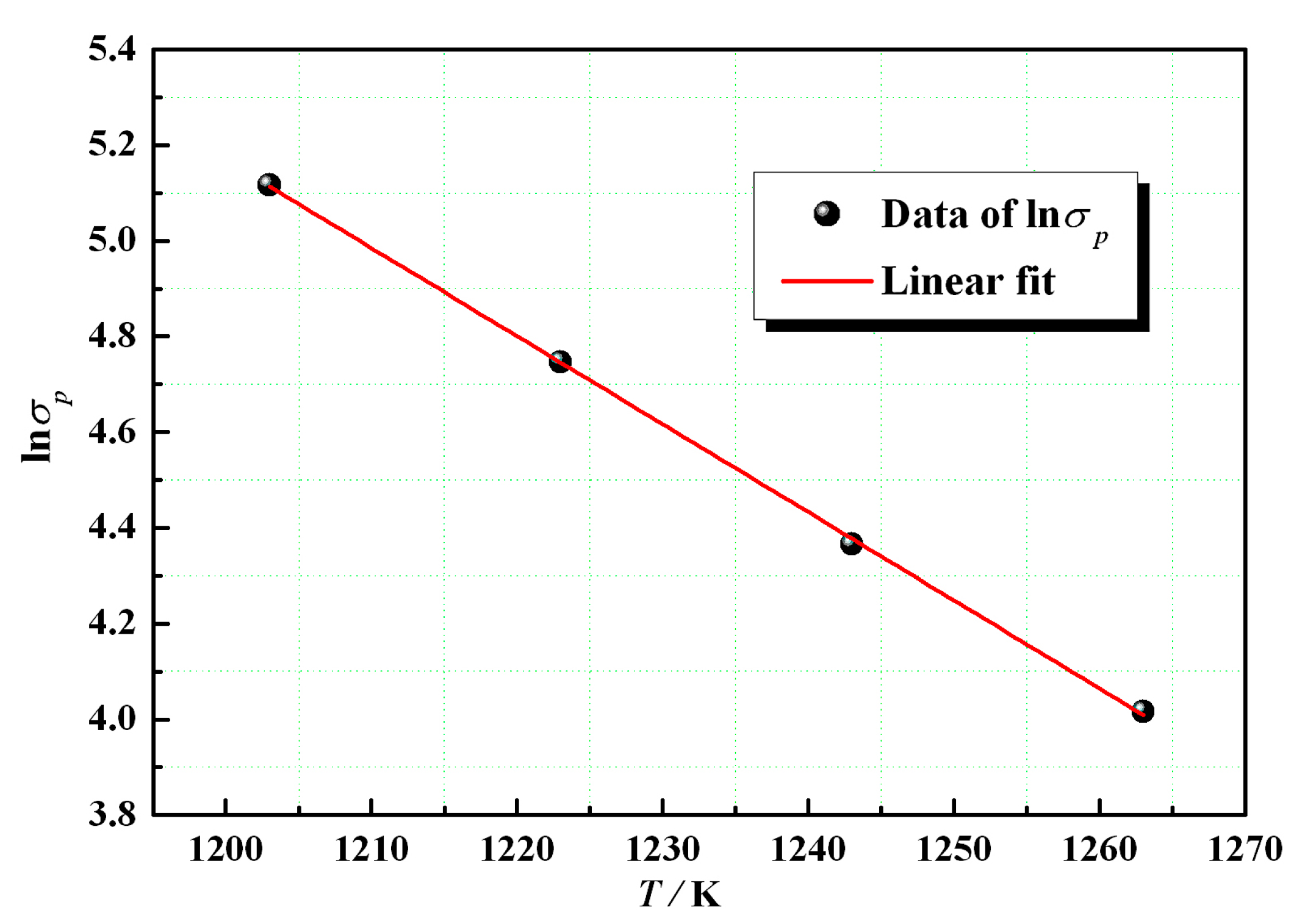
The stress–strain curves at $\dot{\epsilon }=1.0\times {10}^{-3}{\mathrm{s}}^{-1}$ show that the peak stresses σ_p1203 is 166.8 MPa at 930 °C (1203 K) and σ_p1263 is 55.5 MPa at 990 °C (1263 K). Then, Equation (31) can be written as:

$$\ln \left(\frac{{\sigma }_{p1203}-{\sigma }_p}{{\sigma }_{p1203}-{\sigma }_{p1263}}\right)=m\ln \left(\frac{T-1203}{1263-1203}\right)$$

(32)

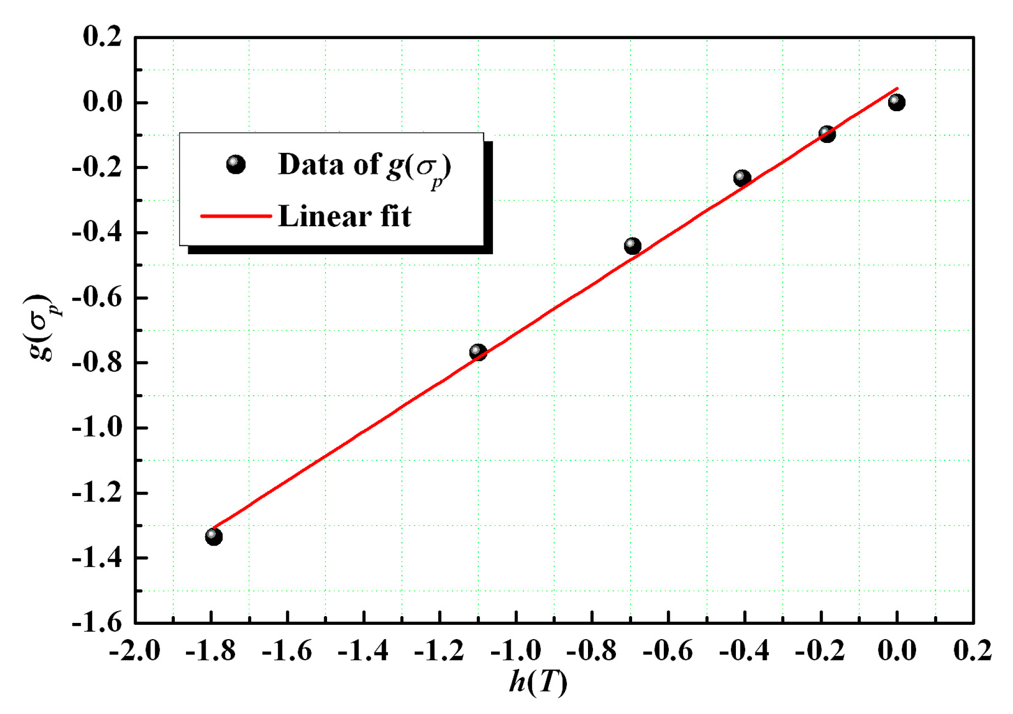
Taking the flow stress at various temperatures into Equation (32), Equation (33) is obtained. The m value is the slope of $g\left({\sigma }_p\right)–h\left(T\right)$ curve, as shown in Figure 6. The value of m is equal to 0.7537 through the linear fitting.

$$\begin{gathered} \ln \left(\frac{166.8-{\sigma }_p}{111.3}\right)=m\ln \left(\frac{T-1203}{60}\right) \\ g\left({\sigma }_p\right)=\ln \left(\frac{166.8-{\sigma }_p}{111.3}\right) \\ h\left(T\right)=\ln \left(\frac{T-1203}{60}\right) \end{gathered}$$

(33)

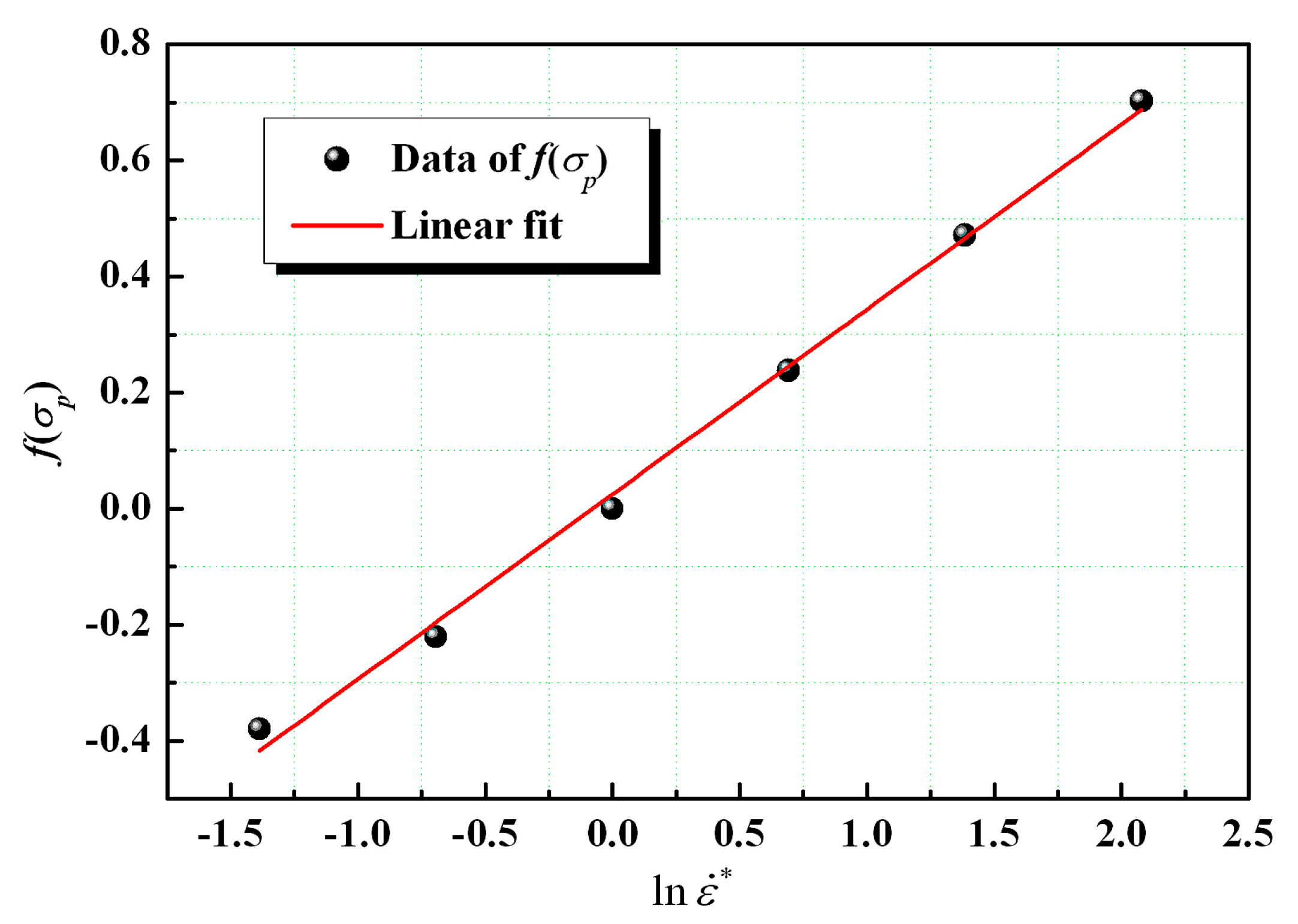
From the stress–strain curves in Figure 1, the peak stress σ_p is 166.8 MPa at T = 930 °C (1203 K) and $\dot{\epsilon }=1.0\times {10}^{-3}{\mathrm{s}}^{-1}$. By taking the peak stress σ_p into Equation (29), Equation (34) can be obtained as below:

$$\begin{gathered} \frac{{\sigma }_p}{166.8}-1=C\ln \dot{\epsilon }* \\ f\left({\sigma }_p\right)=\frac{{\sigma }_p}{166.8}-1 \end{gathered}$$

(34)

The value of C is the slope of $f\left({\sigma }_p\right)–\ln \dot{\epsilon }*$ curve (Figure 7) and equal to 0.3186 by the linear fitting.

Since the referential temperature is 930 °C (1203 K), ${\sigma }_l={\sigma }_{p1203}=166.8$ MPa and ${\sigma }_h={\sigma }_{p1263}=55.5$ MPa in Equation (29) and let T_h = 990 °C (1263 K) replace the melting temperature T_m. Then, taking C and m values into Equation (29), the modified J–C model (Equation (35)) is obtained at temperature range T = 930~990 °C and strain-rate range $\dot{\epsilon }=2.5\times {10}^{-4} ~8\times {10}^{-3}{\mathrm{s}}^{-1}$ with the referential temperature of 930 °C and the referential strain rate of $1.0\times {10}^{-3}{\mathrm{s}}^{-1}$.

$${\sigma }_p=\left(166.8-111.3T{*}^{0.7537}\right)\left(1+0.3186\ln \dot{\epsilon }*\right)$$

(35)

where $\dot{\epsilon }*=\dot{\epsilon }/{\dot{\epsilon }}_0$, ${\dot{\epsilon }}_0=1.0\times {10}^{-3}{\mathrm{s}}^{-1}$, $T*=\left(T-1203\right)/60$. The first bracket represents the softening effect of temperature on the flow stress and the second bracket represents the hardening effect of strain rate on the flow stress. The softening effect of strain on the flow stress can be characterized by introducing a softening factor, which will be introduced later.

If taking the material parameters into the original format of the J–C model in Equation (7), the constitutive equation can be rewritten as:

$${\sigma }_p=166.8\left(1+0.3186\ln \dot{\epsilon }*\right)\left(1-T{*}^{0.7537}\right)$$

(36)

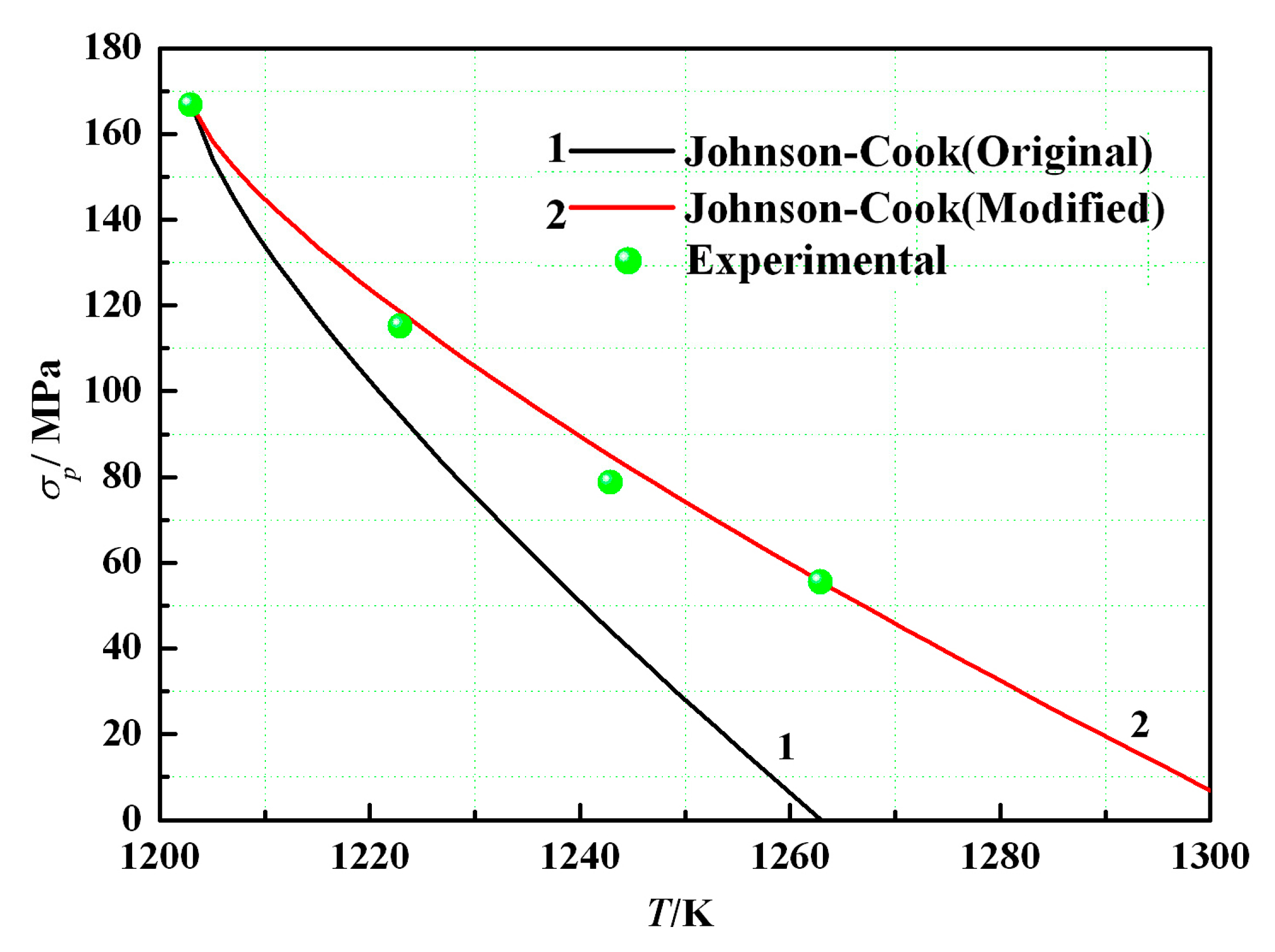
The dependence of peak stress σ_p on temperature obtained from the J–C model in Equations (35) and (36) at a strain rate of 1.0 × 10⁻³ s⁻¹ is shown in Figure 8. Obviously, the fitting of the constitutive equation in Equation (35) exhibits good agreement with the experimental data. In contrast, the constitutive equation depicted in Equation (36) shows a large deviation from the experimental data, indicating that using the improved J–C model to describe the mechanical behavior of some material at a specific temperature range is feasible. However, the original J–C model with the temperature range from the room temperature to melting temperature is not suitable for any deformation condition.

The modification of the J–C constitutive model is useful in investigating the deformation behavior of materials in a specific narrow temperature range, within which the deformation mechanism remains relatively stable. Otherwise, in terms of the original definition of the J–C model, it is unrealistic to use one equation to characterize the material mechanical behavior from the room to melting temperature due to the different deformation mechanism at various temperatures. Therefore, establishing a material constitutive model for various temperature ranges can accurately indicate the influence of temperature on the material deformation behavior. Meanwhile, in most cases, we also focus on the mechanical behavior of material for a certain temperature range. Then, it is extremely important and necessary to establish the material constitutive models in a specific temperature range.

3.4. Comparison and Experimental Verification of Different Constitutive Models

As known from the stress–strain curves, the flow stress of the Ti-22Al-25Nb alloy sheet at elevated temperature is greatly dependent on the temperature, strain rate, and strain. The maximum flow stress, namely peak stress, decreases with increasing temperature and decreasing strain rate. The flow stress increases at the beginning and decreases with the proceeding of straining. In this study, the two kinds of constitutive models were used to quantitatively describe the variation of the flow stress with various influence factors. The Arrhenius model described in Equation (1) shows that the flow stress varies with the strain rate in a hyperbolic sine function and temperature in an exponential function. The J–C model described by Equation (7) shows that the flow stress varies with the strain rate in a logarithmic function and temperature in a power function. The Backofen model described by Equation (4) shows that the flow stress varies with the strain rate in a logarithmic function. Introducing the temperature item $\exp \left(Q/RT\right)$ into the Backofen model (in Equation (4)), it becomes a simplified format of the Arrhenius equation. The difference between the Rosserd model (Equation (5)) and the Backofen model is that the former introduces the strain-hardening item ${\epsilon }^n$ into the latter, which takes both strain and strain-rate hardening into account and is not applicable to the deformation showing strain softening. Therefore, we can introduce such a softening factor $\exp \left(bT\right)\cdot \exp \left(s\epsilon \right)$ or $\exp \left(bT+s\epsilon \right)$ into the Rosserd model to embody the effects of temperature and strain softening on the flow stress. The temperature-softening factor $\exp \left(bT\right)$ is consistent with $\exp \left(Q/RT\right)$ in the Arrhenius model in format and the strain-softening factor $\exp \left(s\epsilon \right)$ can also be applied into other models to describe the strain-softening effect of the flow stress.

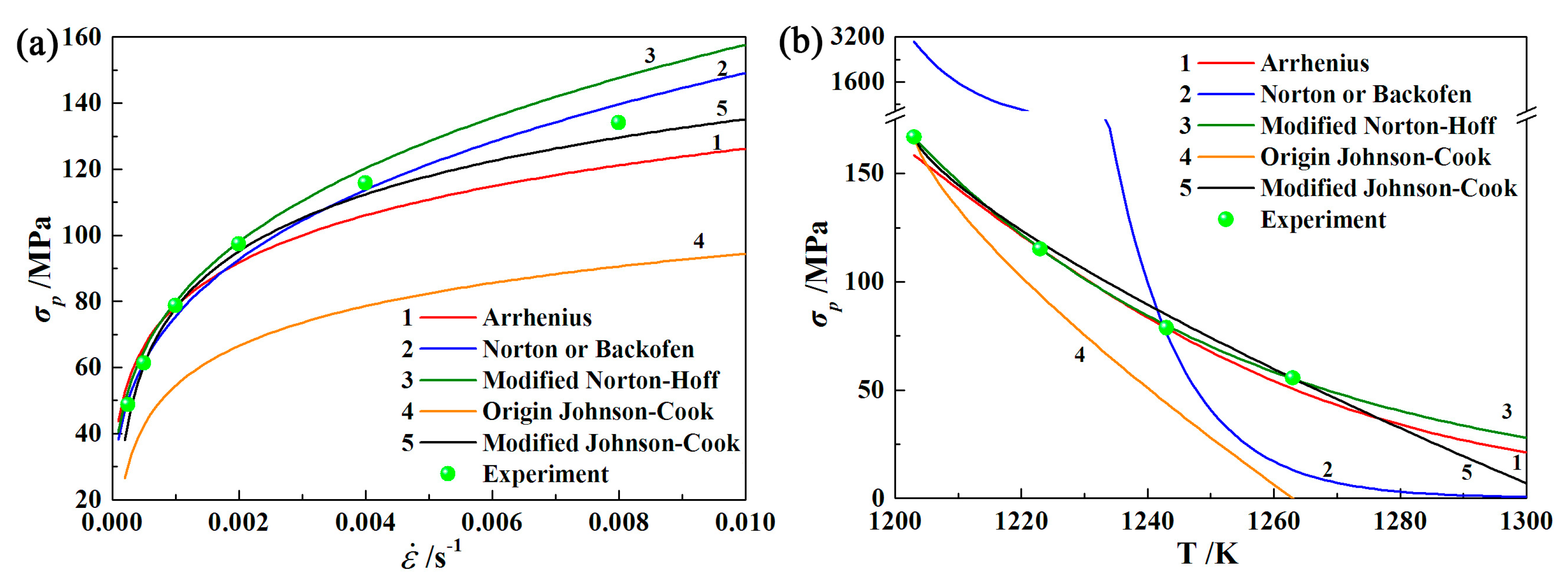
Taking the dependence of peak stress on strain rate at 970 °C, for example, the comparisons between several constitutive models fitting and experimental results are shown in Figure 9a. When the strain rate is low, such as less than 0.001 s⁻¹, the Arrhenius model (including the Norton or Backofen model) is in good agreement with the experimental results. In contrast, when the strain rate is high, such as more than 0.001 s⁻¹, the modified J–C model agrees well with the experimental results. Thus, it can be concluded that the Arrhenius model (including the Norton or Backofen model) is suitable for the deformation with relatively lower strain rates such as the superplastic and creep deformation, and the modified J–C model is suitable for the deformation within a wider range of strain rates. These results are consistent with the initial applications of these models.

Figure 9b shows the comparisons between constitutive models fitting and experimental results of the dependence of peak stress on temperature at the strain rate of 2.5 × 10⁻⁴ s⁻¹ to 8 × 10⁻³ s⁻¹. Computational fitting of both the Arrhenius model and the modified Norton–Hoff model involving softening factor $\exp \left(bT+s\epsilon \right)$ are in good agreement with the experimental results, while the modified J–C model seems to be slightly inferior, indicating that the dependence of the flow stress on temperature follows an exponential function.

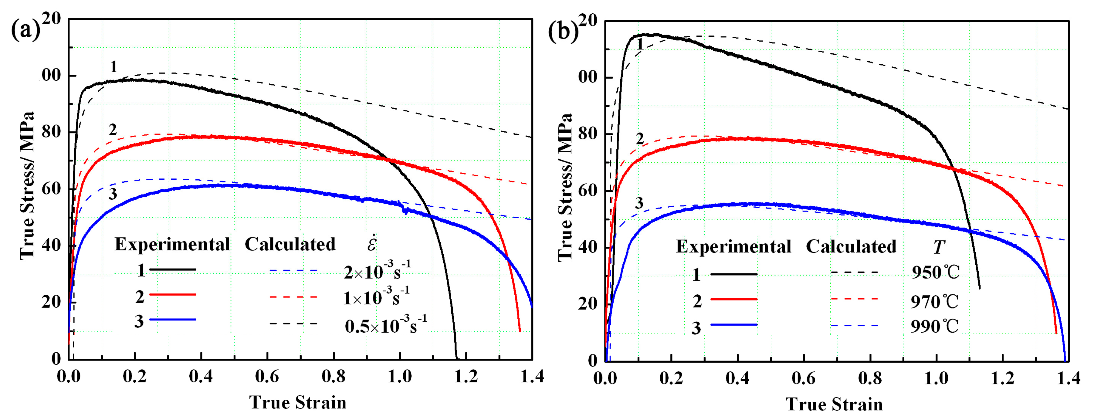
The stress–strain curves obtained from the modified Norton–Hoff constitutive model considering the softening factor (Equation (24)) and experimental results are shown in Figure 10. The calculated curves are in good agreement with the experimental results at condition of T ≥ 970 °C and $\dot{\epsilon }\le 1.0\times {10}^{-3}{\mathrm{s}}^{-1}$, while they have a larger deviation at T < 970 °C, $\dot{\epsilon }>1.0\times {10}^{-3}{\mathrm{s}}^{-1}$. The reason is believed to be that the s value in the softening factor $\exp \left(bT+s\epsilon \right)$ in Equation (19) is calculated based on the deformation at T = 970 °C, $\dot{\epsilon }=1.0\times {10}^{-3}{\mathrm{s}}^{-1}$, which is a constant. However, the experimental stress–strain curves show that the decreasing rate of the flow stress with straining is closely dependent on the deformation temperature and strain rate. Therefore, the s value is a function of the temperature and strain rate, namely $s=f\left(T,\dot{\epsilon }\right)$, rather than a constant. Thus, the deviation is larger at lower temperatures and higher strain rates.

4. Conclusions

The Arrhenius and Johnson–Cook constitutive models for high-temperature deformation of Ti-22Al-25Nb alloys are established using the uniaxial tensile tests, of which the Johnson–Cook model is modified, so that the referential temperature range can be freely adjusted. The Arrhenius model (including the Norton or Backofen model) is suitable for the deformation with relatively lower strain rates such as the superplastic and creep deformation, and the modified J–C model is suitable for the deformation within a wider range of strain rates. For deformation at high temperatures, introducing a strain-softening factor exp(sε) into the constitutive model can describe the flow stress with increasing strain more precisely than the Arrhenius and Johnson–Cook constitutive models.

References

- Wang, D.; Jin, J.; Wang, X. A unified constitutive model for a low alloy steel during warm deformation considering phase differences. J. Mater. Process. Technol. 2017, 245, 80–90. [Google Scholar] [CrossRef]
- Lin, Y.C.; Chen, X.M. A critical review of experimental results and constitutive descriptions for metals and alloys in hot working. Mater. Des. 2011, 32, 1733–1759. [Google Scholar] [CrossRef]
- Lin, Y.C.; Wen, D.-X.; Deng, J.; Liu, G.; Chen, J. Constitutive models for high-temperature flow behaviors of a Ni-based superalloy. Mater. Des. 2014, 59, 115–123. [Google Scholar] [CrossRef]
- Samantaray, D.; Mandal, S.; Bhaduri, A.K. A comparative study on Johnson Cook, modified Zerilli–Armstrong and Arrhenius-type constitutive models to predict elevated temperature flow behaviour in modified 9Cr–1Mo steel. Comp. Mater. Sci. 2009, 47, 568–576. [Google Scholar] [CrossRef]
- Xing, H.L.; Wang, C.W.; Zhang, K.F.; Wang, Z.R. Recent development in the mechanics of superplasticity and its applications. J. Mater. Process. Technol. 2004, 151, 196–202. [Google Scholar] [CrossRef]
- Tsao, L.C.; Wu, H.Y.; Leong, J.C.; Fang, C.J. Flow stress behavior of commercial pure titanium sheet during warm tensile deformation. Mater. Des. 2012, 34, 179–184. [Google Scholar] [CrossRef]
- Guan, Z.; Ren, M.; Zhao, P.; Ma, P.; Wang, Q. Constitutive equations with varying parameters for superplastic flow behavior of Al–Zn–Mg–Zr alloy. Mater. Des. 2014, 54, 906–913. [Google Scholar] [CrossRef]
- Xing, H.L.; Zhang, K.F.; Wang, Z.R. A Study of the Constitutive Equation of Superplastic State. J. Harbin Inst. Technol. 1994, 26, 101–105. [Google Scholar]
- Quan, G.Z.; Liu, K.W.; Zhang, Y.W.; Zhou, J. Rosserd Constitutive Description of Hot Deforming Behavior of AZ80 Magnesium Alloy. Hot Working Technol. 2010, 39, 64–66. [Google Scholar]
- Gavrus, A. Constitutive Equation for Description of Metallic Materials Behavior during Static and Dynamic Loadings Taking into Account Important Gradients of Plastic Deformation. Key Eng. Mater. 2012, 504–506, 697–702. [Google Scholar] [CrossRef]
- Johnson, G.R.; Cook, W.H. A constitutive model and data for metals subjected to large strains, high strain rates and high temperatures. In Proceedings of the 7th International Symposium on Ballistics, Den Haag, The Netherlands, 19–21 April 1983; pp. 541–547. [Google Scholar]
- Prawoto, Y.; Fanone, M.; Shahedi, S.; Ismail, M.S.; Wan Nik, W.B. Computational approach using Johnson–Cook model on dual phase steel. Comp. Mater. Sci. 2012, 54, 48–55. [Google Scholar] [CrossRef] [Green Version]
- Wang, X.; Huang, C.; Zou, B.; Liu, H.; Zhu, H.; Wang, J. Dynamic behavior and a modified Johnson-Cook constitutive model of Inconel 718 at high strain rate and elevated temperature. Mater. Sci. Eng. A 2013, 580, 385–390. [Google Scholar] [CrossRef]
- Ranc, N.; Chrysochoos, A. Calorimetric consequences of thermal softening in Johnson–Cook’s model. Mech. Mater. 2013, 65, 44–55. [Google Scholar] [CrossRef] [Green Version]
- Banerjee, D.; Gogia, A.K.; Nandi, T.K.; Joshi, V.A. A new ordered orthorhombic phase in a Ti3Al-Nb alloy. Acta Metall. 1988, 36, 871–882. [Google Scholar] [CrossRef]
- Banerjee, D. The intermetallic Ti2AlNb. Prog. Mater. Sci. 1997, 42, 135–158. [Google Scholar] [CrossRef]
- Gavrus, A. Formulation of a new constitutive equation available simultaneously for static and dynamic loadings. In Proceedings of the 9th International Conference on the Mechanical and Physical Behavior of Materials under Dynamic Loading, Brussels, Belgium, 7–11 September 2009; pp. 1239–1244. [Google Scholar]
Figure 1.
Stress–strain curves for the initial sheet: (a) various temperatures and ; (b) various strain rates at 970 °C.
Figure 2.
Relationship of: (a) vs. ; (b) vs. .
Figure 3.
Plot of vs. at .
Figure 4.
Graph of σp-(, T) function at , T = 930~990 °C.
Figure 5.
Plot of vs. at and T = 930~990 °C.
Figure 6.
Figure 7.
Plot of vs. at T = 970 °C and .
Figure 8.
Variation of σp with temperature at for the two J–C models.
Figure 9.
Variation of the peak stress of each constitutive model: (a) different strain rates and T = 970 °C; (b) different temperatures and .
Figure 10.
Comparison between experimental and calculated stress–strain curves: (a) different strain rates and T = 970 °C; (b) different temperatures and .
© 2019 by the authors. Licensee MDPI, Basel, Switzerland. This article is an open access article distributed under the terms and conditions of the Creative Commons Attribution (CC BY) license (http://creativecommons.org/licenses/by/4.0/).
Share and Cite
MDPI and ACS Style
He, Z.; Wang, Z.; Lin, P. A Comparative Study on Arrhenius and Johnson–Cook Constitutive Models for High-Temperature Deformation of Ti2AlNb-Based Alloys. Metals 2019, 9, 123. https://doi.org/10.3390/met9020123
AMA Style
He Z, Wang Z, Lin P. A Comparative Study on Arrhenius and Johnson–Cook Constitutive Models for High-Temperature Deformation of Ti2AlNb-Based Alloys. Metals. 2019; 9(2):123. https://doi.org/10.3390/met9020123
Chicago/Turabian StyleHe, Zhubin, Zhibiao Wang, and Peng Lin. 2019. "A Comparative Study on Arrhenius and Johnson–Cook Constitutive Models for High-Temperature Deformation of Ti2AlNb-Based Alloys" Metals 9, no. 2: 123. https://doi.org/10.3390/met9020123
Note that from the first issue of 2016, this journal uses article numbers instead of page numbers. See further details here.