Article

Numerical Simulation of Three-Dimensional Mesoscopic Grain Evolution: Model Development, Validation, and Application to Nickel-Based Superalloys

State Key Laboratory of Materials Processing and Die & Mould Technology, Huazhong University of Science and Technology, Wuhan 430074, China
*
Author to whom correspondence should be addressed.
Metals 2019, 9(1), 57; https://doi.org/10.3390/met9010057
Submission received: 27 November 2018 / Revised: 2 January 2019 / Accepted: 5 January 2019 / Published: 9 January 2019
(This article belongs to the Special Issue Numerical Modelling and Simulation of Metal Processing)

Abstract

:
The mesoscopic grain model is a multiscale model which takes into account both the dendrite growth mechanism and the vast numerical computation of the actual castings. Due to the pursuit of efficient computation, the mesoscopic grain calculation accuracy is lower than that of dendrite growth model. Improving the accuracy of mesoscopic grain model is a problem to be solved urgently. In this study, referring to the calculation method of solid fraction in microscopic dendrite growth model, a cellular automata model of 3D mesoscopic grain evolution for solid fraction calculated quantitatively at the scale of cell is developed. The developed model and algorithm validation for grain growth simulation is made by comparing the numerical results with the benchmark experimental data and the analytical predictions. The results show that the 3D grain envelopes simulated by the developed model and algorithm are coincident with the shape predicted by the analytical model to a certain extent. Then, the developed model is applied to the numerical simulation of solidification process of nickel-based superalloys, including equiaxed and columnar dendritic grain growth. Our results show good agreement with the related literature.

1. Introduction

Grain evolutions including nucleation and growth during solidification process have a profound effect on the material mechanical properties of alloys. In particular, the competitive growth of equiaxed and columnar dendritic grains determine the microstructure of alloys. Over the past few decades, many computer models and methods have been developed to study theoretically and experimentally the grain growth in alloy solidification, such as the volume-averaged, front tracking, cellular automata (CA), and phase field models [1,2,3,4,5]. Among them, due to the advantages of clearly describing the physical phenomena and high computational efficiency of solidification transition, the CA model has been widely used and developed for prediction of grain growth in additive manufacturing [6,7], welding [8,9], and casting [10,11].
In 1993, the CA model was applied for the first time in alloy solidification by Rappaz and Gandin [12]. It mainly dealt with nucleation and growth of grains in a uniform temperature field. At this point, the basic framework of the CA model for grain growth simulation was constructed, although it still had some drawbacks. Subsequently, in order to satisfy the adaptability of non-uniform temperature field at the same time, the “2D rectangular algorithm” [13] and “decentered square algorithm” [14,15] coupled with finite element (FE) calculations were proposed. Similarly, the CA model could also be coupled with the finite difference (FD) method to form the CA-FD model [16], or coupled with the finite volume (FV) method to form the CA-FV model [17]. As one of the effective methods to simulate the growth of grain, the CA-FE model integrated into the casting commercial software of ProCAST have been widely used [18,19].
However, the growing octahedron in these models is no longer considered if the corresponding cell is fully surrounded by the mushy cells [15]. In this way, this CA-FE model is still a weak coupling method and overestimates the heat release of cell transformation in the mushy zone [20]. In the CA model, the solid fraction of growing cell or interface cell in the mushy zone cannot be calculated quantitatively at the scale of CA grid. And it is calculated approximately at the scale of FE grid by the Scheil’s equation and the Scheil microsegregation model. Recently, Guillemot et al. [20] have employed a front tracking method proposed by Gandin [21] to deal with the coupling problem. Similar works have also been conducted by Carozzani et al. [22] and Liu et al. [23,24].
Additionally, the CA model of grain growth, ignoring the dendritic morphology of the grain itself, is generally referred to as mesoscopic model. Corresponding CA models of dendritic growth called microscopic model have been proposed and developed, typically works like Nastac’s [25], Zhu’s [26] and Pan’s [27]. In this regard, it is a full coupling model that accounts for the time evolution of the fraction of solid predicted at the scale of CA grid in the CA model of dendritic growth. It is further observed in the CA models of two scales that both are faced with the same problems of grid anisotropy [13,28], transformation rules [14,29], and coupling methods [30]. From the point of view of the simulation method, the method for dealing with the same problem in the CA models of two scales are interrelated [16,31]. Nevertheless, there is a problem that the CA model of dendritic growth requires sufficiently higher mesh resolution than the CA model of grain growth [32].
The purpose of this paper is to achieve the full coupling simulation of grain growth so as to improve the simulation accuracy. A 3D modified cellular automaton coupling model of grain growth for solid fraction calculated quantitatively at the scale of CA gird is proposed. The relevant models and algorithms are presented and validated. Then, the developed model is applied to simulate the formation of equiaxed and columnar dendritic grains during solidification process of nickel-based superalloys.

2. Model Description and Numerical Algorithm

A 3D computation domain is firstly divided into a series of regular hexahedral cells. The cell spacing is equal to the corresponding mesh size. Each cell is characterized with such variables as solid fraction, grain growth rate, grain orientation, etc. All the cell states are defined as three types: liquid (fs = 0), solid (fs = 1), or interface (0 < fs <1). And the cell neighbors are characterized by the first-order neighbors (6 neighborhoods), second-order neighbors (12 neighborhoods), and third-order neighbors (8 neighborhoods). At the beginning of the numerical simulation, the cells in computation domain are initialized with given initial and boundary conditions. When the undercooling reaches or exceeds the critical nucleation undercooling, the grain begins to nucleate and grow. As the dendritic grain grows, the solid fraction of growing cell or interface cell is calculated quantitatively at the scale of CA grid. The governing equations for calculating the nucleation distribution and growth rate of dendritic grains are presented. The numerical algorithm about capture rules for new interface cells and the calculation of solid fraction at the scale of CA grid are described in detail below.

2.1. Grain Nucleation

Only heterogeneous nucleation is considered in this study, since high undercooling is not achieved due to the presence of foreign phases. For the sake of practicability, the continuous nucleation model proposed by Rappaz and Gandin et al. [12] is used to describe the grain nucleation. The total grain density nT) is calculated by:
n ( Δ T ) = 0 Δ T d n d Δ T d ( Δ T )
where ΔT is the undercooling.
The continuous nucleation distribution dn/dΔT′ is given by:
d n d Δ T = n max 2 π Δ T σ exp [ 1 2 ( Δ T Δ T N Δ T σ ) ]
where nmax is the total density of grains, ΔTσ is the standard deviation of undercooling, and ΔTN is the mean undercooling in nucleation, respectively. Additionally, the total density of grains on the two-dimensional section (nmax)2D can be obtained by the stereological relationships [12], (nmax)2D = (6·nmax2/π)1/3.
Unlike the numerical realization of nucleation process determined by random number method, in this present study, the nucleation position and critical undercooling are randomly assigned to the nucleation region in advance, and then the actual undercooling and the critical undercooling of each cell are compared in each time step to determine the nucleation.

2.2. Grain Growth

Grain growth rate is mainly determined by the growth behavior of dendrite tips. According to the Lipton-Glicksman-Kurz (LGK) growth model [33,34], the dendrite tips growth of alloys are affected by thermal undercooling (ΔTt), constitutional undercooling (ΔTc) and curvature undercooling (ΔTR). With the growth of dendrite tips, latent heat and solute are released from tips. At the interface of dendrite tips, heat and solute transfer lead to changes in thermal and constitutional undercooling. In addition, the growth of dendrite tips also lead to the change of curvature undercooling. At a given total undercooling, the grains will grow under the interaction of various factors until they grow up completely or encounter obstacles to stop growth.
The thermal undercooling, constitutional undercooling and curvature undercooling are defined as:
Δ T t = I v ( P t ) Δ H c p
Δ T c = m L C 0 ( 1 1 1 ( 1 k 0 ) I v ( P c ) )
Δ T R = 2 Γ R
where Iv(P) is the Ivantsov function of the Peclet number; Pt = RV/(2α) and Pc = RV/(2D) are the heat Peclet number and solutal Peclet number, respectively; ΔH is the latent heat; cp is the specific heat; mL is the liquidus slope; C0 is the initial components concentration of alloys; k0 is the solute partition coefficient; Γ is Gibbs-Thompson coefficient; R is the tip radius; V is the interface growth rate; α is thermal diffusion coefficient; and D is solute diffusion coefficient.
The 3D Ivantsov function is expressed as:
I v ( P ) = P exp ( P ) E 1 ( P )
where E1(P) is the exponential integral function.
The relationship between the tip radius and the interface growth rate can be established by combining the above equations, but it cannot be solved, and other more definite conditions are needed.
Based on the stability criterion of a dendrite tip, the tip radius is equal to the shortest wavelength λi, which can be evaluated by:
λ i = ( Γ σ * ( m L G c G ) ) 0.5
where Gc is the concentration gradient; G is the temperature gradient; σ* is a stability parameter, it should be noted here that the stability parameter according to the microsolvability theory varies with the degree of anisotropy of the interface energy, and its value can be obtained by the linearized solvability theory [35].
For ease of numerical calculations, the above equations are realized and solved using Matlab. The growth rate is simplified as a polynomial function of local undercooling.

2.3. Capture Rules for New Interface Cells and Calculation of Solid Fraction at the Scale of the CA Grid

A single regular octahedron is defined as a constituent element of a grain. Each cell corresponds to a regular octahedron. The sizes of regular octahedrons are characterized by the distance (SL) between any two adjacent vertices. Its three orthogonal axes ([100]/[010]/[001]) represent the directions of dendrite tips. Meanwhile, in order to avoid the infinite growth problem of the single regular octahedron, the distance (SL) is limited to 2·Δxx is the cell size). The grain envelope, which consists of a number of regular octahedrons, is also shown as a larger regular octahedron in the uniform temperature field. A single grain whose crystallographic orientation is assumed to be the Euler angles (φ, θ, ψ) with respect to the axis of CA, as shown in Figure 1.
In this present work, the nucleated cell is defined as a solid cell. And all its neighbor cells are defined as interface cells with a solid fraction of ε (ε→0). When the solid fraction of the interface cells reaches 1 or greater than 1, all the first-order, second-order, and third-order neighbors’ liquid cells of the former interface cell transform to interface cells. At this point, it is guaranteed that at least one of the 26 neighbor cells of the interface cells evolves to a solid cell. The Schematic diagram of cell state is shown in Figure 2. For the octahedron corresponding to the nucleated cell, the center of octahedron coincides with the center of nucleated cell. While the center of octahedron corresponding to the interface cell also coincides with the center of nucleated cell. Similar to 3D decentered square algorithm, the tips length of octahedron (L) from its center to any of its six vertices are given by:
L ( t 2 ) = L ( t 1 ) + t 1 t 2 V ( Δ T ( τ ) ) d τ
where t2 represents the next time, t1 represents the current time. The initial tip length of the grain corresponding to the nucleated cell is taken as the maximum value (√2·Δx). The initial tip length of the grain corresponding to the interface cell is taken as ε (ε→0).
During the evolution of grains, due to the displacement between the center of the interface cell and the center of the growing octahedron, the growing octahedron corresponding to the interface cell will capture the cell center of the neighbors of solid cell. When the interface cell is captured, it is then switched to the solid cell. At this moment, all the remaining liquid cells being neighbors of this new solid cell will be automatically transferred from liquid to interface cells. The new octahedron corresponding to this new interface cell is initialized. Once the tip length of the growing octahedron is equal to or greater than the maximum value (√2·Δx), the growing octahedron will cease to grow. The corresponding interface cell will be switched to the solid cell regardless of the solid fraction of the interface cell.
In order to realize the self-consistency between the tip length of the growing octahedron and the solid fraction of interface cell, a quantitative method for calculating the two is described below.
Figure 3 and Figure 4 sketch the capture rule for solid cell in a time step calculation. When the center of growing octahedron corresponding to the interface cell (for example, IJ) coincides with the center of nucleated cell, the fraction increment of the interface cell IJ is calculated by:
Δ f s = Δ L L 1 w i t h    L 1 2 Δ x
where ΔL represent the increment of the tip length of the growing octahedron, L1 represent the final tip length (OA1) of the growing octahedron.
Subsequently, as soon as the center of the interface cell IJ is captured by the growing octahedron, this interface cell is immediately switched to solid cell and the remaining liquid cells adjacent to this new solid cell will be transformed into new interface cells (for example, IJK), as shown in Figure 4. As mentioned above, the new growing octahedron corresponding to the new interface cell IJK is initialized. Especially, the center (O0) of the new growing octahedron is also located at the center of the octahedron corresponding to the original interface cell IJ. And the tip length of the new growing octahedron is initialized with the maximum value Lm (Lm = √2·Δxε). As a result, before the solid fraction of the new interface cell IJK reaches 1, the center (O2) of the new growing octahedron has moved gradually along the direction of growth so as to maintain its continuous growth. In this case, the fraction increment of the new interface cell IJK is calculated by:
Δ f s = Δ L L 2 L m
where L2 represent the final tip length (O0A3) of the growing octahedron.

3. Results and Discussion

3.1. Comparison with the Benchmark Experimental Data

Firstly, to validate the numerical calculation program for mesoscopic grain growth in this study, the dendritic tip growth rate of a succinonitrile-acetone mixtures are calculated and compared with benchmark experimental data [34]. According to the microsolvability theory, the stability parameter remains unchanged within a certain range of Peclet number. Here, two stability parameters are considered. Figure 5 presents the dendritic tip growth rate as a function of initial concentration in succinonitrile-acetone mixtures.
As shown in Figure 5, under both undercooling conditions of 0.5 K and 0.9 K, the dendrite tip growth rate calculated by numerical methods increases first and then decreases with the initial concentration, which is consistent with the experimental results. For the initial concentration range of 0–0.25 (mol. %), the curve of the dendritic tip growth rate with a stability parameter of 0.025 is approximately matched with the experimental results. For the initial concentration range of 0.25–0.45 (mol%), the curve of the dendritic tip growth rate with a stability parameter of 0.0195 is approximately matched with the experimental results. It is confirmed that the stability parameters match the experimental results only in a certain range of Peclet numbers.

3.2. Comparison with the Analytical Model of Grain Growth

The model and algorithm validation for grain growth simulation is made by comparing the numerical results with the analytical model predictions [14,36]. In the analytical growth model, it was assumed that the grain growth was controlled by the solute diffusion and only applicable to the low Peclet number regime. This is basically similar to the assumption of the LGK model. There are two kinds of grain branches predicted by the analytical model, here the external envelope is assumed to be the grain envelope. Figure 6 presents the schematic diagram of two-dimensional dendrite growth envelope trajectory under directional temperature. In the process of two-dimensional dendritic growth under directional solidification, the coordinates of the external envelope trajectory can be calculated by Equation (11) [36]:
{ x = x 0 + ( y y 0 ) f ( θ ) Δ T = Δ T L g ( θ ) h ( G A Δ T L g ( θ ) ( t t 0 ) ) + Δ T 0 g ( θ ) Δ T L 1 + S 10 Δ T 0 g ( θ ) Δ T L h ( G A Δ T L g ( θ ) ( t t 0 ) ) y = v L t Δ T G
where VL is the moving rate of liquid isotherm, ΔTL is the dendrite tip undercooling, ΔT0 is the undercooling at initial time t0, θ is the dendrite orientation angle, A is a constant coefficient in LGK model, f(θ), g(θ) and S<10> are directional functions related to the orientation angle respectively, which are given by Equations (12)–(14).
{ f ( θ ) = 1 tan ( θ ) for   the   [ 10 ]   and   [ 1 ¯ 0 ]   branches f ( θ ) = tan ( θ ) for   the   [ 01 ]   and   [ 0 1 ¯ ]   branches
{ g ( θ ) = sin ( θ ) for   the   [ 10 ]   and   [ 1 ¯ 0 ]   branches g ( θ ) = cos ( θ ) for   the   [ 01 ]   and   [ 0 1 ¯ ]   branches
{ S 10 = 1 for   the   [ 10 ]   and   [ 01 ]   branches S 10 = 1 for   the   [ 1 ¯ 0 ]   and   [ 0 1 ¯ ]   branches
Since the above analytical model is based on two-dimensional dendrite growth, it is necessary to extend this method to three-dimensional grain growth. In this present study, the projection method and the three cosine theorem are used to calculate the outermost envelope trajectory of a three-dimensional grain. Besides, since the analytical model was restricted to a quadratic approximation of the velocity-undercooling relationship, the growth rate was temporarily simplified as the same quadratic approximation relationship of local undercooling in the numerical simulation. Figure 7 presents the 3D envelopes and tips length of a single grain growing in a uniform temperature field and in a Bridgman-like situation. In Figure 7a, the cooling rate is set to 0 K/s and the thermal gradient is set to 0 K/m, the tips length (L1, L2, L3, L4, L5, L6) of the grain corresponding to Figure 7a are shown in Figure 7b. In Figure 7c, the cooling rate is set to −0.1 K/s and the thermal gradient along the Z-axis is set to 250 K/m, the tips length (L1, L2, L3, L4, L5, L6) of the grain corresponding to Figure 7c are shown in Figure 7d. The cell size Δx is set to 0.0001 m.
As shown in Figure 7a,c the 3D views of analytical and numerical predictions, for a given crystallographic orientation, are approximately regular octahedrons in a uniform temperature field. In Bridgman-like situations, due to the effects of deep undercooling, the tips length (L4, L6) of the grain closest to the negative thermal gradient direction are the longer distances. Altogether, the 3D grain envelopes (a2, c2) simulated by the developed model and algorithm in both cases are visually reproduced and coincident with the shape (a1, c1) predicted by the analytical model. Furthermore, from the Figure 7b,d, it can be noted that there are only a few mesh size gaps among the tips length of the grain in both predictions, which also approximately present the same distribution.

3.3. Model Application to Nickel-Based Superalloys

The present model is used to simulate the formation of equiaxed and columnar dendritic grains during nickel-based superalloys solidification process. The elemental composition (mass fraction, wt.%) of the material is Ni–7.82Cr–5.34Co–2.25Mo–4.88W–6.02Al–1.94Ti–3.49Ta. For multicomponent alloys, a large number of simplifications and calculations are required due to the complex multicomponent coupling solidification process. Here, a multicomponent pseudo-binary alloy method [37] is used. The material properties and model parameters used in these simulations are listed in Table 1.

3.3.1. Equiaxed Dendritic Grains

The calculation domain is uniformly divided into 200 × 200 × 200 meshes with mesh size of 0.0001 m. It is assumed that the temperature field is homogeneous and cooled down from liquidus temperature at different cooling rates leading to nucleation and growth process. The cooling rates are set to 1 K·s−1, 10 K·s−1, and 100 K·s−1, respectively. Here, the nucleation process only takes into account the nucleation inside the melt. It must be stressed that the nucleation parameters are affected by many factors, such as random nucleation, solidification conditions, etc. It cannot be uniquely determined or calculated in advance. For the ease of numerical calculations, the nucleation parameter is assumed to be known in advance. In the bulk of the melt, the total density of grains is 1 × 10¹⁰ m−3, the median undercooling is 3 K, and the standard deviation of undercooling is 0.5 K. Figure 8 presents the size distribution of equiaxed dendritic grains at different cooling rates.
Figure 8 shows that, with the increase of cooling rate, the grain size of equiaxed grains decreases obviously, and the grain density increases from 0.13 mm−2 to 4.08 mm−2. From the data analysis of the two-dimensional section, it can be seen that the number of grains approximately presents a normal distribution curve at d/<d> from 0 to 2.0. With higher cooling rates the maximum of the grain number as function of d/<d> grows, while its dispersion in grain-size lowers. The highest grain number-density is always given close to the median grain-size. It is indicated that the increase of cooling rate can significantly promote the grain refinement. These results are consistent with the experimental results of solidification microstructures [38], which preliminarily validate the effectiveness of the proposed model and algorithm.

3.3.2. Columnar Dendritic Grains

Cooling rate and temperature gradient are two important parameters for directional solidification microstructure. Since the thermal diffusion rate is more than several orders of magnitude larger than the solute diffusion rate, it can be assumed that the temperature is uniform at the scale of a grain. At a fixed temperature gradient (G) and cooling rate (C) the temperature isotherms of the whole calculation domain will change at the same drawing speed (R = C/G). The calculation domain is uniformly divided into 60 × 180 × 600 cubic cells with size of 0.0001 m. Two types of nucleation parameters are considered. At the bottom surface, the total density of grains is 5.0 × 10⁵ m−3, the mean undercooling is 0 K, and the standard deviation is 0 K. In the bulk of the melt, the total density of grains is 1 × 10¹⁰ m−3, the mean undercooling is 3 K, and the standard deviation is 0.5 K.

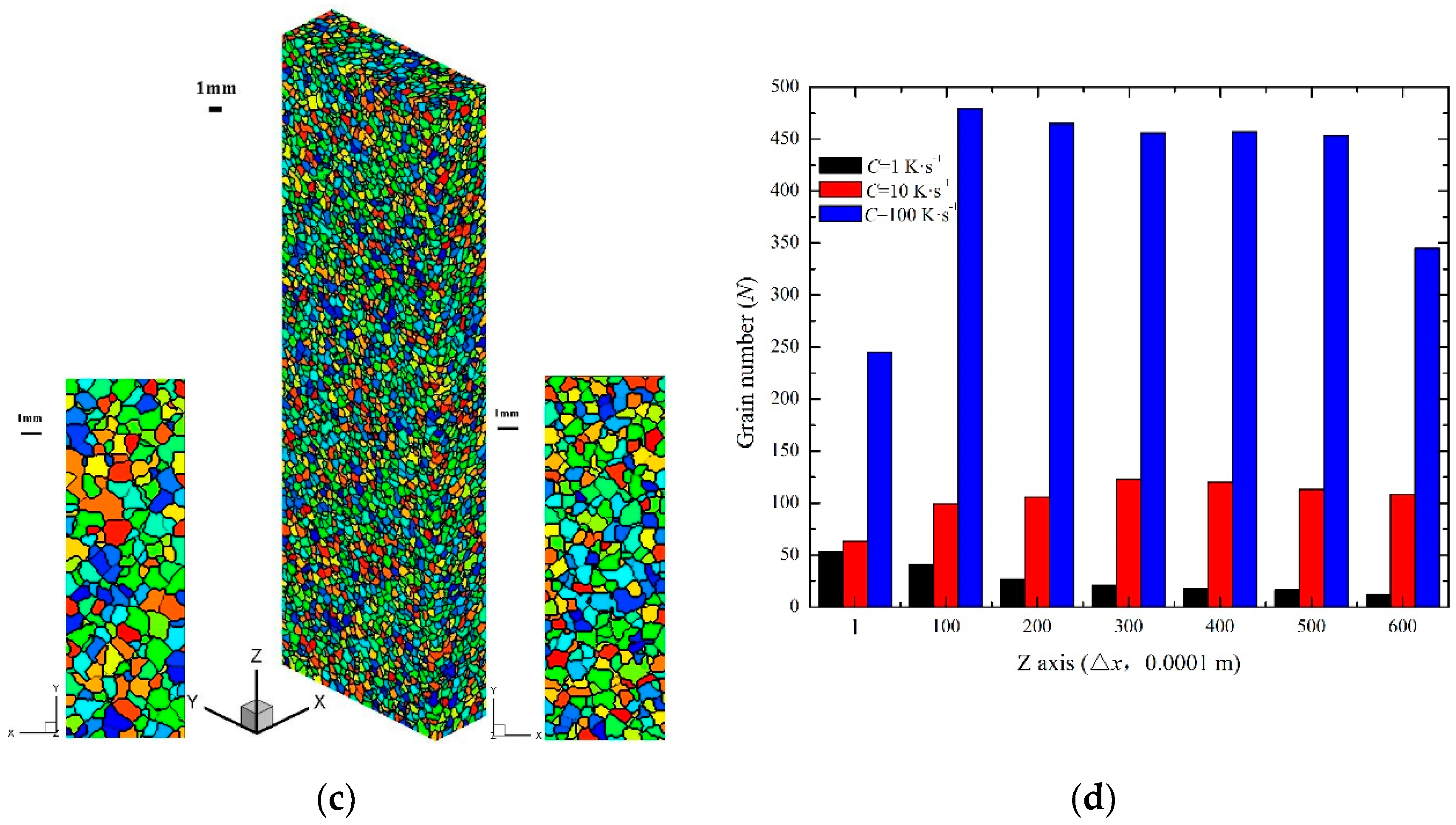
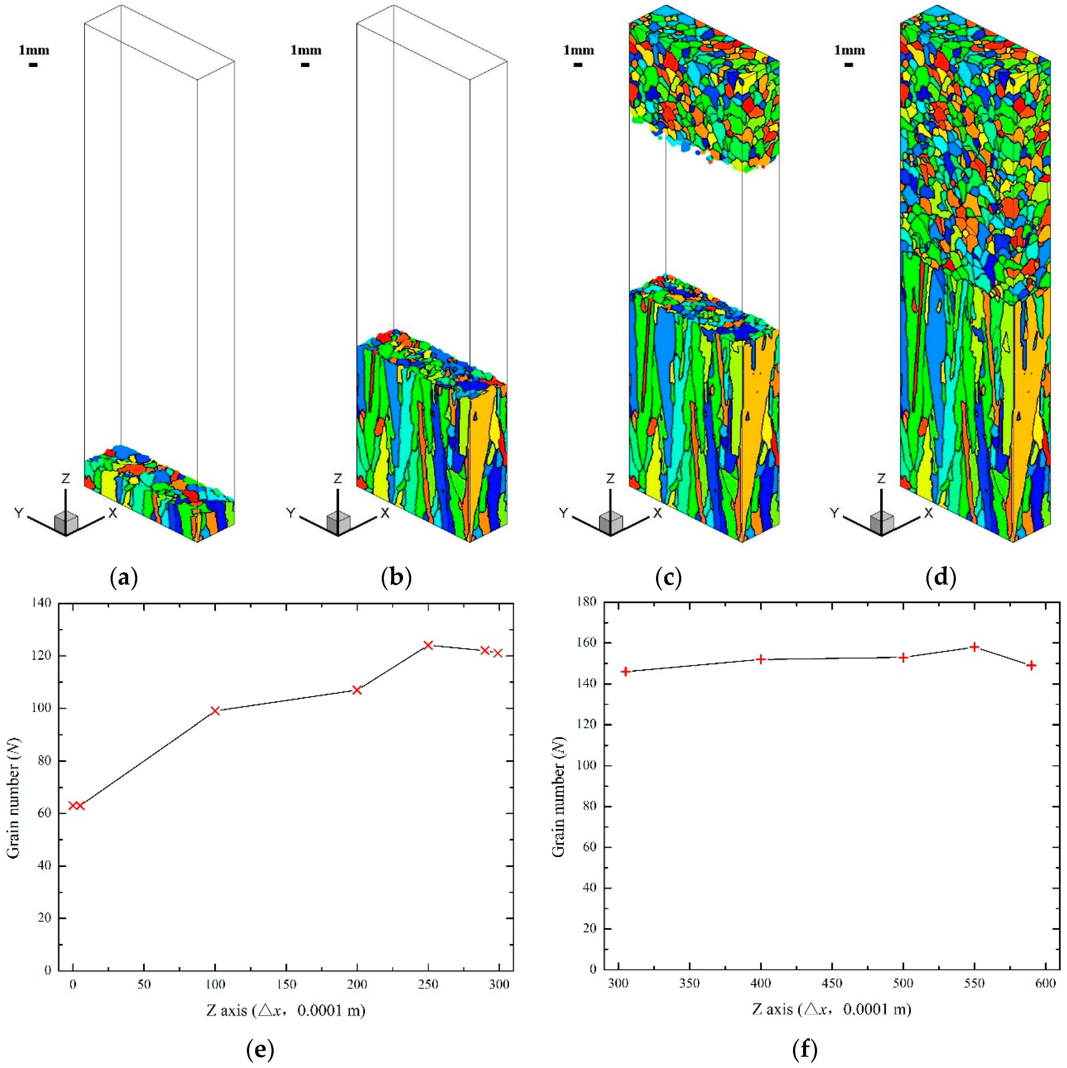
Equiaxed-to-Columnar Transformation (ECT) for Different Cooling Rates

The temperature gradient is set to 1000 K·m−1. And the cooling rates are set to 1 K·s−1, 10 K·s−1, and 100 K·s−1, respectively. Figure 9 presents the grain size distributions for different cooling rates.
Figure 9 shows, that for different cooling rates, the developed solidification microstructures of the calculated domain gradually changes (with respect to the size distribution of grains). At the cooling rate of 1 K·s−1, some thick columnar dendritic grains are shown in the calculation domain, and the number of grains decreases gradually along the Z axis. At the cooling rate of 10 K·s−1, the grain structure in the calculation domain is composed of both columnar and fine equiaxed dendritic grains, and the number of grains increases first and then decreases. At the cooling rate of 100 K·s−1, almost all grains in the calculation domain are small equiaxed dendritic grains, and the number of grains increases suddenly and decreases slowly with increasing Z. From the above results, it can be inferred that at low cooling rate the grain growth rate of directional solidification is faster than the grain nucleation rate in the supercooled region of melt. In addition, due to the boundary limitation of the calculation domain, some grains deviating from the direction of temperature gradient will be eliminated at the boundary, resulting in the gradual decrease of the number of grains along the Z axis.

Equiaxed-to-Columnar Transformation (ECT) for Different Temperature Gradients

The temperature gradient is set to 500 K·m−1, 1000 K·m−1, and 1500 K·m−1, respectively. The cooling rates are set to 10 K·s−1. Figure 10 presents the grain size distributions for different temperature gradients.
Figure 10 shows for the calculated domain, that with increasing temperature gradient, the solidification microstructure develops to the opposite of the results presented in Figure 8. In other words, at the temperature gradient of 500 K·m−1, almost all grains in the calculation domain are small equiaxed dendritic grains, and the number of grains increases suddenly and decreases slowly. At the temperature gradient of 1500 K·m−1, some thick columnar dendritic grains are shown in the calculation domain, and the number of grains decreases gradually along the Z axis. It can also be deduced that a rapid growth of columnar dendritic grains is promoted more by an increasing temperature gradient than by an increasing nucleation rate.

3.3.3. Columnar-to-Equiaxed Transformation (CET)

The ECT and CET are common phenomena of the grain evolution in solidification process. Under different solidification conditions, the transformations rule of the two influences the grain size distribution in the casting. During directional solidification, the ECT transformation is beneficial to the growth of columnar dendritic grains, and it is also affected by the nucleation parameters and cooling rate. Since the cooling rate and the temperature gradient are difficult to control, the casting of the metallic alloy may exhibit a non-uniform distribution of the temperature field. Especially, when the temperature gradient gradually decreases to a negative temperature gradient, this will lead to the CET transformation. To characterize the positive-to-negative transition in the temperature gradient, the temperature gradient is set to 1000 K·m−1 from mesh point 0 to 300 in the direction of the Z axis, and the temperature gradient is set to −300 K·m−1 from mesh point 300 to 600 in the direction of the Z axis. The cooling rate is set to 10 K·s−1. The other grain nucleation and growth parameters set here are the same as those above Section 3.3.2. Figure 11 presents the simulation results of the CET transformation.
As shown in Figure 11, in the calculation domain, the grains first nucleate and grow at the bottom surface. From mesh point 0 to 300 in the direction of the Z axis, under the positive temperature gradient, grains begin to compete with each other along the Z axis, which is similar to the ECT transformation process mentioned above. From mesh point 300 to 600 in the direction of the Z axis, the grains nucleate and grow at the top surface under the negative temperature gradient. Compared with the ECT transformation process, the grains grow in the form of a large number of equiaxed crystals. Finally, the two parts of the grain stop growing at intermediate position, thus forming the CET transformation process. The above results show a good agreement with the results of related literature [23,39,40], which further validates the applicability of the proposed model and algorithm.

4. Conclusions

A cellular automata model of 3D mesoscopic grain evolution is developed. In this model, the 3D grain envelope trajectory is coupled with the solid fraction in a cell. The solid fraction in grain growth is calculated quantitatively at the scale of a CA grid. The detailed model and algorithm validations are performed by comparing the numerical results with the analytical model predictions. The simulated 3D grain envelopes are found to be in agreement with the analytical predictions. The developed model was then applied to simulate the formation of equiaxed and columnar dendritic grains during the solidification process of nickel-based superalloys. The results of this simulation could well explain the evolution law of grain growth in solidification microstructures, including equiaxed dendritic grain growth, columnar dendritic grain growth, and microstructure transformation.
Although the mesoscopic grain growth in a simple temperature field is studied in this present work, the proposed grain envelope trajectory coupled with the cell solid fraction method can be easily extended to complex multiscale and multiphysical field calculations. Such a 3D mesoscopic grain model coupled to a macroscopic temperature field and solute field is in progress and can be used to simulate the solidification process of actual castings.

Author Contributions

Z.G. and J.Z. wrote the paper; Z.G. and Y.Y. did the simulations; Z.G. and X.S. analyzed the data; Z.G. and X.J. revised the paper.

Funding

This work was supported by the National Natural Science Foundation of China (No. 51605174, No. 51775205) and AECC Beijing Institute of Aeronautical Materials.

Conflicts of Interest

The authors declare no conflicts of interest.

References

  1. Wu, M.; Ludwig, A. A three-phase model for mixed columnar-equiaxed solidification. Metall. Mater. Trans. A 2006, 37, 1613–1631. [Google Scholar] [CrossRef]
  2. Satbhai, O.; Roy, S.; Ghosh, S. A parametric multi-scale, multiphysics numerical investigation in a casting process for Al-Si alloy and a macroscopic approach for prediction of ECT and CET events. Appl. Therm. Eng. 2017, 113, 386–412. [Google Scholar] [CrossRef]
  3. Mcfadden, S.; Browne, D.J.; Gandin, C.A. A comparison of columnar-to-equiaxed transition prediction methods using simulation of the growing columnar front. Metall. Mater. Trans. A 2009, 40, 662–672. [Google Scholar] [CrossRef]
  4. Martorano, M.A.; Biscuola, V.B. Predicting the columnar-to-equiaxed transition for a distribution of nucleation undercoolings. Acta Mater. 2009, 57, 607–615. [Google Scholar] [CrossRef]
  5. Souhar, Y.; Felice, V.F.D.; Beckermann, C.; Combeau, H.; Založnik, M. Three-dimensional mesoscopic modeling of equiaxed dendritic solidification of a binary alloy. Comput. Mater. Sci. 2016, 112, 304–317. [Google Scholar] [CrossRef] [Green Version]
  6. Lopez-Botello, O.; Martinez-Hernandez, U.; Ramírez, J.; Pinna, C.; Mumtaz, K. Two-dimensional simulation of grain structure growth within selective laser melted AA-2024. Mater. Des. 2017, 113, 369–376. [Google Scholar] [CrossRef]
  7. Tian, F.; Li, Z.; Song, J. Solidification of laser deposition shaping for TC4 alloy based on cellular automation. J. Alloys Compd. 2016, 676, 542–550. [Google Scholar] [CrossRef]
  8. Chen, S.; Guillemot, G.; Gandin, C.A. Three-dimensional cellular automaton-finite element modeling of solidification grain structures for arc-welding processes. Acta Mater. 2016, 115, 448–467. [Google Scholar] [CrossRef]
  9. Valvi, S.R.; Krishnan, A.; Das, S.; Narayanan, R.G. Prediction of microstructural features and forming of friction stir welded sheets using cellular automata finite element (CAFE) approach. Int. J. Mater. Form. 2016, 9, 115–129. [Google Scholar] [CrossRef]
  10. Zhang, Q.; Xue, H.; Tang, Q.; Pan, S.Y.; Rettenmayr, M.; Zhu, M.F. Microstructural evolution during temperature gradient zone melting: Cellular automaton simulation and experiment. Comput. Mater. Sci. 2018, 146, 204–212. [Google Scholar] [CrossRef]
  11. Hu, Y.; Xie, J.; Liu, Z.; Ding, Q.; Zhu, W.; Zhang, J.; Zhang, W. CA method with machine learning for simulating the grain and pore growth of aluminum alloys. Comput. Mater. Sci. 2018, 142, 244–254. [Google Scholar] [CrossRef]
  12. Rappaz, M.; Gandin, C.A. Probabilistic modelling of microstructure formation in solidification processes. Acta Metall. Mater. 1993, 41, 345–360. [Google Scholar] [CrossRef]
  13. Gandin, C.A.; Rappaz, M. A coupled finite element-cellular automaton model for the prediction of dendritic grain structures in solidification processes. Acta Metall. Mater. 1994, 42, 2233–2246. [Google Scholar] [CrossRef]
  14. Gandin, C.A.; Rappaz, M. A 3D cellular automaton algorithm for the prediction of dendritic grain growth. Acta Mater. 1997, 45, 2187–2195. [Google Scholar] [CrossRef]
  15. Gandin, C.A.; Desbiolles, J.L.; Rappaz, M.; Thevoz, P. A three-dimensional cellular automation-finite element model for the prediction of solidification grain structures. Metall. Mater. Trans. A 1999, 30, 3153–3165. [Google Scholar] [CrossRef]
  16. Wang, W.; Lee, P.D.; Mclean, M. A model of solidification microstructures in nickel-based superalloys: Predicting primary dendrite spacing selection. Acta Mater. 2003, 51, 2971–2987. [Google Scholar] [CrossRef]
  17. Zhu, M.F.; Hong, C.P. A Three Dimensional Modified Cellular Automaton Model for the Prediction of Solidification Microstructures. Trans. Iron Steel Inst. Jpn. 2002, 42, 520–526. [Google Scholar] [CrossRef]
  18. Pozdniakov, A.N.; Monastyrskiy, V.P.; Ershov, M.Y.; Monastyrskiy, A.V. Simulation of competitive grain growth upon the directional solidification of a Ni-base superalloy. Phys. Met. Metallogr. 2015, 116, 67–75. [Google Scholar] [CrossRef]
  19. Carter, P.; Cox, D.C.; Gandin, C.A.; Reed, R.C. Process modelling of grain selection during the solidification of single crystal superalloy castings. Mater. Sci. Eng. A 2000, 280, 233–246. [Google Scholar] [CrossRef]
  20. Guillemot, G.; Gandin, C.A.; Combeau, H.; Heringer, R. A new cellular automaton—finite element coupling scheme for alloy solidification. Model. Simul. Mater. Sci. Eng. 2004, 12, 545–556. [Google Scholar] [CrossRef]
  21. Gandin, C.A. From constrained to unconstrained growth during directional solidification. Acta Mater. 2000, 48, 2483–2501. [Google Scholar] [CrossRef]
  22. Carozzani, T.; Digonnet, H.; Gandin, C.A. 3D CAFE modeling of grain structures: Application to primary dendritic and secondary eutectic solidification. Model. Simul. Mater. Sci. Eng. 2012, 20, 15010–15028. [Google Scholar] [CrossRef]
  23. Liu, D.R.; Mangelinck-noël, N.; Gandin, C.A.; Zimmermann, G.; Sturz, L.; Nguyen-Thi, H.; Billia, B. Structures in directionally solidified Al–7 wt.% Si alloys: Benchmark experiments under microgravity. Acta Mater. 2014, 64, 253–265. [Google Scholar] [CrossRef]
  24. Liu, D.R.; Mangelinck-noël, N.; Gandin, C.A.; Zimmermann, G.; Sturz, L.; Nguyen-Thi, H.; Billia, B. Simulation of directional solidification of refined Al–7 wt.% Si alloys–Comparison with benchmark microgravity experiments. Acta Mater. 2015, 93, 24–37. [Google Scholar] [CrossRef]
  25. Nastac, L. Numerical modeling of solidification morphologies and segregation patterns in cast dendritic alloys. Acta Mater. 1999, 47, 4253–4262. [Google Scholar] [CrossRef]
  26. Zhu, M.F.; Stefanescu, D.M. Virtual front tracking model for the quantitative modeling of dendritic growth in solidification of alloys. Acta Mater. 2007, 55, 1741–1755. [Google Scholar] [CrossRef]
  27. Pan, S.Y.; Zhu, M.F. A three-dimensional sharp interface model for the quantitative simulation of solutal dendritic growth. Acta Mater. 2010, 58, 340–352. [Google Scholar] [CrossRef]
  28. Beltran-Sanchez, L.; Stefanescu, D.M. A quantitative dendrite growth model and analysis of stability concepts. Metall. Mater. Trans. A 2004, 35, 2471–2485. [Google Scholar] [CrossRef]
  29. Reuther, K.; Rettenmayr, M. Perspectives for cellular automata for the simulation of dendritic solidification–A review. Comput. Mater. Sci. 2014, 95, 213–220. [Google Scholar] [CrossRef]
  30. Zhu, M.F.; Pan, S.Y.; Sun, D.K.; Zhao, H.L. Numerical simulation of microstructure evolution during alloy solidification by using cellular automaton method. ISIJ Int. 2010, 50, 1851–1858. [Google Scholar] [CrossRef]
  31. Chen, R.; Xu, Q.; Liu, B. Cellular automaton simulation of three-dimensional dendrite growth in Al–7Si–Mg ternary aluminum alloys. Comput. Mater. Sci. 2015, 105, 90–100. [Google Scholar] [CrossRef] [Green Version]
  32. Zinovieva, O.; Zinoviev, A.; Ploshikhin, V.; Romanova, V.; Balokhonov, R. A solution to the problem of the mesh anisotropy in cellular automata simulations of grain growth. Comput. Mater. Sci. 2015, 108, 168–176. [Google Scholar] [CrossRef]
  33. Kurz, W.; Giovanola, B.; Trivedi, R. Theory of microstructural development during rapid solidification. Acta Metall. 1986, 34, 823–830. [Google Scholar] [CrossRef]
  34. Lipton, J.; Glicksman, M.E.; Kurz, W. Dendritic growth into undercooled alloy metals. Mater. Sci. Eng. 1984, 65, 57–63. [Google Scholar] [CrossRef]
  35. Barbieri, A.; Langer, J.S. Predictions of dendritic growth rates in the linearized solvability theory. Phys. Rev. A 1989, 39, 5314–5325. [Google Scholar] [CrossRef]
  36. Gandin, C.A.; Schaefer, R.J.; Rappax, M. Analytical and numerical predictions of dendritic grain envelopes. Acta Mater. 1996, 44, 3339–3347. [Google Scholar] [CrossRef]
  37. Stefanescu, D.M. Science and Engineering of Casting Solidification, 3nd ed.; Springer: Cham, Switzerland, 2015; pp. 145–196. [Google Scholar]
  38. Kavoosi, V.; Abbasi, S.M.; Ghazi Mirsaed, S.M.; Mostafaei, M. Influence of cooling rate on the solidification behavior and microstructure of IN738LC superalloy. J. Alloys Compd. 2016, 680, 291–300. [Google Scholar] [CrossRef]
  39. Mishra, S.; DebRoy, T. Non-isothermal grain growth in metals and alloys. Mater. Sci. Technol. 2006, 22, 253–278. [Google Scholar] [CrossRef]
  40. Spittle, J.A. Columnar to equiaxed grain transition in as solidified alloys. Int. Mater. Rev. 2006, 51, 247–269. [Google Scholar] [CrossRef]
Figure 1. Schematic diagram of a single regular octahedron with arbitrary orientation (φ, θ, ψ).
Metals 09 00057 g001
Figure 2. Schematic diagram of the cell state.
Metals 09 00057 g002
Figure 3. Schematic diagram of the capture rule for solid cell in a time step calculation, the center of IJ is in the final plane A1D1E1 of the growing octahedron with L1 ≤ √2·Δx.
Metals 09 00057 g003
Figure 4. Schematic diagram of the capture rule for solid cells in a time step calculation, the center of IJK is in the final plane A3D3E3 of the growing octahedron with Lm = √2·Δxε.
Metals 09 00057 g004
Figure 5. Dendritic tip growth rate as a function of initial concentration in succinonitrile-acetone mixtures.
Metals 09 00057 g005
Figure 6. Schematic diagram of two-dimensional dendrite growth envelope trajectory under directional temperature.
Metals 09 00057 g006
Figure 7. 3D envelopes and tips length of a single growing grain at time t = 7 s after nucleation, where the grain is assumed to nucleate and grow with an initial undercooling ΔT0 = 2 K, the crystallographic orientation (20°, 40°, 60°) and the growth constant A = 0.0001 m/(s·K2). (a) 3D envelopes in a uniform temperature field; (b) tip length in a uniform temperature field; (c) 3D envelopes in a Bridgman-like situation; and (d) tip length in a Bridgman-like situation.
Metals 09 00057 g007
Figure 8. Size distribution of equiaxed dendritic grains at different cooling rates. (a) Simulation results of three-dimensional equiaxed dendritic grains; and (b) size distribution of equiaxed dendritic grains in a two-dimensional section.
Metals 09 00057 g008aMetals 09 00057 g008b
Figure 9. Grain size distributions for different cooling rates. (a) C = 1 K·s−1; (b) C = 10 K·s−1; (c) C = 100 K·s−1; and (d) grain number along the Z axis.
Metals 09 00057 g009aMetals 09 00057 g009b
Figure 10. Grain size distributions for different temperature gradients. (a) G = 500 K·m−1; (b) G = 1000 K·m−1; (c) G = 1500 K·m−1; and (d) grain number along the Z axis.
Metals 09 00057 g010
Figure 11. CET transformation. (a) t = 0.5 s; (b) t = 2.0 s; (c) t = 2.7 s; (d) t = 3.3 s; (e) grain number (0 ≤ Z ≤ 300); and (f) grain number (300 ≤ Z ≤ 600).
Metals 09 00057 g011
Table 1. Material properties and model parameters.
ParametersValue
Density (kg·m3)7223.48
Specific heat (J·(kg·K)−1)1074.60
Thermal conductivity (W·(m·K)−1)37.43
Latent heat (J·kg−1)23,3371.59
Initial equivalent concentration of solute (wt.%)31.74
Equivalent coefficient of partition (wt.%)0.57
Equivalent slope of liquidus−1.96
Gibbs Thomson Coefficient (K·m)1.0 × 10⁻⁷
Solute diffusion coefficient in the liquid (m2·s−1)3.0 × 10⁻⁹
Solute diffusion coefficient in the solid (m2·s−1)3.0 × 10⁻¹²

