Stochastic Material Point Method for Analysis in Non-Linear Dynamics of Metals


1
College of Aerospace and Civil Engineering, Harbin Engineering University, Harbin, Heilongjiang 150001, China
2
Inner Mongolia First Machinery Group CO., LTD., Baotou, Inner Mongolia 014000, China
*
Author to whom correspondence should be addressed.
Metals 2019, 9(1), 107; https://doi.org/10.3390/met9010107
Submission received: 20 December 2018
/
Revised: 9 January 2019
/
Accepted: 18 January 2019
/
Published: 21 January 2019
Abstract
:A stochastic material point method is proposed for stochastic analysis in non-linear dynamics of metals with varying random material properties. The basic random variables are parameters of equation of state and those of constitutive equation. In conjunction with the material point method, the Taylor series expansion is employed to predict first- and second-moment characteristics of structural response. Unlike the traditional grid methods, the stochastic material point method does not require structured mesh; instead, only a scattered cluster of nodes is required in the computational domain. In addition, there is no need for fixed connectivity between nodes. Hence, the stochastic material point method is more suitable than the stochastic method based on grids, when solving dynamics problems of metals involving large deformations and strong nonlinearity. Numerical examples show good agreement between the results of the stochastic material point method and Monte Carlo simulation. This study examines the accuracy and convergence of the stochastic material point method. The stochastic material point method offers a new option when solving stochastic dynamics problems of metals involving large deformation and strong nonlinearity, since the method is convenient and efficient.
1. Introduction
The traditional grid methods have been successfully employed for several decades in engineering practice but has limitations when the considered non-linear dynamics problem of metals involves large deformation, such as hyper-velocity impact and explosion, due to distortions in the mesh when implementing a Lagrangian approach. The deformation of the grids can lead to numerical inaccuracies or even render the calculation impossible [1,2]. To overcome these difficulties, a great number of meshless methods—such as the smoothed particle hydrodynamics method [3,4], the diffuse element method [5], the element-free Galerkin method [6,7], partition of unity [8], the reproducing kernel particle method [9,10], the cracking particles [11], the dual-horizon peridynamics [12,13] and the material point method (MPM) [14,15,16]—have been proposed and developed in recent years to solve non-linear dynamics problems of metals [17,18].
Among these methods, MPM shows many advantages in tension stability and efficiency [19,20,21,22]. Compared with the traditional grid methods, MPM is specifically intriguing because of its simplicity, which have proven useful for solving solid mechanics problems involving large deformation and strong nonlinearity, such as hyper-velocity impact and explosion. [23,24,25,26,27]. MPM can be classified as a meshless method, inheriting the advantages of both Eulerian and Lagrangian methods. Hence, MPM avoids the mesh distortion in the Lagrangian methods and the convection problems in the Eulerian methods [28,29]. To date, MPM and its extensions have been applied successfully to explosion problems [30], impact and penetration problems [1,31,32], fluid-solid interaction problems [33,34] and so on. However, all of the developments in MPM have so far focused on deterministic problems. Probabilistic models using MPM have not received much attention. Furthermore, the stochastic analysis of non-linear dynamics problem involves large deformation and strong nonlinearity, such as hyper-velocity impact and explosion; depends mainly on Monte Carlo simulation, which has disadvantages of low calculating efficiency; and is not naturally suitable for complex engineering practice [35]. Hence, high-efficiency stochastic analysis involving MPM provides a rich, relatively unexplored field for future research [36].
This paper proposes a stochastic material point method (SMPM) for stochastic analysis in non-linear dynamics metal structure with varying random material properties. The samples of basic random variables are parameters of equation of state and those of constitutive equation. In conjunction with the MPM, the Taylor series expansion is employed to predict first- and second-moment characteristics (mean and variance) of structural response. Two numerical examples based on non-linear problems of steel are carried out to examine the accuracy and convergence of the proposed method.
2. Stochastic Material Point Method
The main idea of the SMPM is to introduce the stochastic theory into MPM to make stochastic analysis of non-linear dynamics. Thus, the SMPM has similar features to MPM. In the SMPM, the continuum body is divided into a set of infinitesimal mass elements and these infinitesimal mass elements are represented by a finite collection of material particles, as shown in Figure 1.
The governing equations of continuous materials are standard conservation equations for mass and momentum
where ρ is the mass density, is the velocity, σ is the Cauchy stress tensor and b is the body force per unit mass.
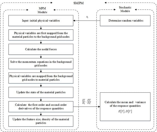
The key steps for SMPM, of which includes the coupling between MPM module and stochastic module and the return of the needed response quantities are illuminated in Figure 2. The following detailed steps are performed at each time step increment Δt:
The first step is to input initial physical variables and at the same time, random variables are passed to the MPM module from the stochastic module.
The second step is mapping velocity and mass of the particles to the background grid nodes with the shape functions. The concrete forms are
where is the position vector of the particle at time , is the nodal velocity at time , is the particle velocity at time , is the shape function for node , is the nodal mass at time and is the particle mass.
The third step is calculating the nodal forces, the internal force vector and the external force vector . The concrete forms are
where is the vectors of prescribed surface traction, is the stress boundary condition, .is the density of the material particle at time , is the stress tensor of the material particle at time and is the body force of the material particle at time .
The forth step is solving the momentum equation in the background grid nodes. The concrete form is
where is the momentum of the node at time t and .is the momentum of the node at time .
The fifth step is to map the information from the background grid nodes back to the material particles. The velocity and displacement vectors of the material particles are mapped from the background grid nodes.
For history-dependent materials, it is convenient to carry strain and stress as well as history variables along with the material particles. Hence, the sixth step is to update the state of the material particles. The information of strain and stress can be updated with the constitutive equation and equation of state and the variables of strain, stress and pressure will be discussed in Section 3. Meanwhile, the first-order and second-order derivative of the response quantities are calculated and passed to the stochastic module from the MPM module. Then, the mean and variance of the response quantities are calculated in the stochastic module and the content of random analysis will be presented in Section 4.
The seventh step is to update the feature size and density of the material particles. The concrete forms are
where is feature size of the material particle at time in the direction , is feature size of the material particle at time in the direction , is the strain increment in the direction and is the density of the material particle at time .
The eighth step is resetting the background grid elements to the original undeformed state.
This completes the computational cycle of a time step. Repeat steps 2–8 until the time has advanced to the desired value.
3. Material Property Equations
3.1. Equation of State
One century ago, Mie [37] and Grüneisen [38] developed a theory for metals which concluded that the pressure could be considered as a linear function of internal energy. The name Mie-Grüneisen is now associated to an equation of state which verifies this assumption. The Mie-Grüneisen equation of state is conveniently couched in an enthalpy framework, which contains two states of the materials defined by the index μ. And μ > 0 represents the compressed state, μ < 0 represents the expanded state. The concrete form is
where is the pressure of a metal, S1, S2, S3, γ0 and a are constants, ρ0 is the original value of the density and e is the internal energy of a metal. The index μ is defined as .
3.2. Constitutive Equation
In general, the response of metals under high-speed impact conditions involves consideration of effects of strain, strain rate and temperature. The Johnson-Cook plasticity model [39,40,41] is employed to model the flow stress behavior of ductile materials. The Johnson-Cook model represents the Von Mises flow stress σy as a function of some parameters as follows
where εP is equivalent plastic strain, is equivalent plastic strain rate, A, B, C and m are constants, n is strain hardening exponent and is homologous temperature defined as
where T is the material temperature, Tmelt is the melting temperature and Troom is the room temperature.
3.3. Von Mises Elastic-Plastic Material Model
Von Mises yield model can be used to describe the plastic behavior of metal materials [42]. The Von Mises elastic-plastic model can be used to describe deviatoric stress update procedure and the radial return mapping can be used at the same time. Under the assumption that the metal materials are in elastic state, the trial deviatoric stress tensor can be calculated by
where is increment of the deviatoric strain, is the deviatoric stress tensor after the rotation, the superscript n is the previous iteration step at the same time step and the superscript n + 1 is the current iteration step at the same time step.
At this moment, the trial Von Mises flow stress can be calculated by
If the following condition holds , the deviatoric stress is in the yield surface. And the trial deviatoric stress tensor acts as the deviatoric stress tensor .
If the following condition holds , the deviatoric stress is beyond the yield surface. Therefore, should be reduced scale representation with the purpose of making it in the yield surface, the concrete form as follows
where the coefficient m can be calculated as
Considering Equations (13) and (15), the plastic strain increment can be calculated as
Considering Equations (14) and (16), the equivalent plastic strain increment is
The flow stress of Von Mises isotropic hardening materials can be updated by
where H is the plastic modulus.
By substituting of Equations (17) and (20) into Equation (18), the equivalent plastic strain increment can be calculated by
In a word, the calculation procedures of Von Mises elastic-plastic material model are summarized as follows
- Calculate the trial deviatoric stress tensor and the trial Von Mises flow stress .
- If the condition holds, the equivalent plastic strain increment can be calculated by Equation (20). Otherwise, the materials have no plastic deformation.
- Update equivalent plastic strain by .
- Update flow stress by Equation (19), get .
- Calculate the coefficient m with the new flow stress by Equation (16) and update the deviatoric stress which satisfies the condition in the yield surface with the radial return mapping.
4. Random Method
4.1. The Basic Random Variables and Random Response
To introduce random parameters to describe the random characteristics of materials is one of the most important factors in stochastic analysis. The random parameters include parameters of equation of state, constitutive equation and those introduced to establish stochastic modeling by defining basic random variables . Therefore, information for random variables must be provided, such as the mean , the variance and the correlation coefficient between two random variables .
The direct solution of structural response is challenging, as it comprises multidimensional integral and the structural response is denoted by . A possible solution to overcome this issue is approximating the structural response via an expression that is an explicit function of the basic random variables. Consequently, introducing the powerful technique of expansion is necessary to calculate first- and second-moment characteristics (mean and variance) of structural response [43], such as, Neumann series expansion [44], polynomial chaos expansion [45] and Taylor series expansion [46,47,48]. It is the first attempt to apply MPM in the field of stochastic analysis and this study is focused on applying the new method in stochastic mechanics and thus, Taylor series expansion has been employed because of its simple and convenient.
In order to calculate the approximation for first-moment of the structural response, assume is expressed in terms of its corresponding second order Taylor series expansion about the point . The concrete form is calculated as follows
where is the remainder of second order Taylor series expansion.
Magnitude analysis proved that the remainder has a relatively weak intensity compared to the first-three terms of Taylor series expansion and hence, the influence of the remainder on deformation of the structure can be neglected. Calculating the mean of both sides of Equation (21) gives the mean of the structural response as follows
In a similar way, in order to calculated the approximation for the second-moment characteristics of structural response, assume is expressed in terms of its corresponding first order of the Taylor series expansion about the point . The concrete form is calculated as follows
where is the remainder of first order Taylor series expansion.
Similarly, the variance of the structural response can be calculated by
The Taylor series expansion is applied to stochastic analysis while meeting certain conditions. If the variation coefficient is less than about 0.2 or 0.3, a better approximation can be obtained by using the first-two terms of the Taylor series expansion. Further, the condition is widened in approximation by using the first-three terms of the Taylor series expansion [49]. The first-moment characteristics of structural response can be obtained through the first-three term of the Taylor series expansion; correspondingly, the second-moment characteristics can be obtained from the first-two terms of the Taylor series expansion. Additionally, probabilistic convergence studies of second order stochastic perturbation technique show that the second order method cannot be used for the coefficient of variation larger than 0.15 to determine efficiently higher order statistics [43,50,51,52,53]. To avoid the obvious errors, a variation coefficient of no larger than 0.15 is selected for this paper. Meanwhile, through comparison with the Monte Carlo method, the reasonableness and correctness of the Taylor series expansion described in this paper will be proved through two concrete instances in Section 5.
Substituting concrete forms into Equation (22) and (24), then we can reach the stochastic structural response after rearranging.
Considering Equation (10) in Section 3.1, the mean and variance of the pressure can be calculated by
Considering Equation (11) in Section 3.2 and the relationship between σy and in Section 3.3, the mean and variance of the equivalent plastic stress and the deviatoric stress can be calculated by
where is the operation of the mean, is the operation of the variance.
4.2. The First-Order and Second-Order Derivatives of the Response Quantities
The first- and second-order derivatives of the response quantities with respect to the random input parameters are involved in Equations (25–28). The estimation of these derivatives is a key problem in stochastic analysis, which is discussed as follows. Suppose the parameters of Mie-Grüneisen equation of state model and those of Johnson-Cook plasticity model are random variables, such as S1, S2, S3, γ0, a, A, B, C, m and n.
If μ > 0, the derivatives in Equations (25) and (26) can be calculated by
where B1, B2, B3 and B4 are defined as follows
If μ < 0, the derivatives in Equations (25) and (26) can be calculated by
The derivatives in Equations (27) and (28) can be calculated by
where C1, C2, C3, C4, C5 and C6 are defined as follows
5. Results and Discussion
Two numerical examples based on steel with different stochastic parameters under explosive force are presented, in which the determined values of the parameters for steel are employed according to ref. [54]. These examples involve not only large deformation but also multi-field coupling, in which the uncertain parameters are all subject to normal distribution. In the first example, the uncertain parameters are the Mie-Grüneisen equation of state with respect to parameters , , , γ0 and . In the second example, the uncertain parameters are the Johnson–Cook parameters , , , and . The probability distribution and correlation structure of the random properties should be defined through experimental measurements. However, in most cases, it is difficult to obtain the random material properties via experimental measurements. Hence, due to the lack of relevant experimental data, assumptions are made regarding these probabilistic characteristics. The Gaussian assumption is often used due to its simplicity and the lack of relevant experimental data in lots of research [35,55,56,57,58] and thus, it is adopted in this study because the focus of this paper is stochastic analysis in non-linear dynamics problem of metals with the SMPM. In practical applications, dependent random variables are often generated by some transformation of independent random variables, so it is assumed without much loss of generality that the components of the random variables, which mentioned in this study, are independent [59]. Hence, the correlation coefficient between two random variables is 0.
Both the stochastic material point method and Monte Carlo simulation are used to calculate the mean and variance of structural response. Monte Carlo simulation is used as a validation tool. Notably, Monte Carlo simulation requires generating N random samples to guarantee result precision. Estimating N is based on the relationship between the confidence interval and sample size [60,61]. Hence, with 95% confidence degree, the sample size is 10000, which can meet the precision requirement of the two numerical examples. All calculations are processed on a personal computer with a 3.30 GHz processer and 8 GB of RAM. The calculated results are described as follows.
5.1. Example 1: The Uncertain Parameters are the State Equation Parameters
The computational domain is full of water with 2 m × 2 m × 2 m dimensions. A thick steel plate of 2 m × 2 m × 0.06 m dimensions is mounted within the domain, with the clamped edge condition assumed. TNT is a cuboid of 0.08 m × 0.08 m × 2 m dimensions and mounted on one side of the plate. Because of symmetry, the analogy model can be further simplified as a 2D planar model, as shown in Figure 3. To better monitor the stochastic response, two points, E and F, of the plate are chosen. Table 1 shows the locations of points E and F of the plate. The situations of the coefficient of variation (C.V) 0.01 and 0.05 are under consideration and the values of the parameters are given in Table 2.
Particles distribution at the end time is shown in Figure 4. The result shows the characteristics of large deformation and multi-field coupling. Using the proposed stochastic material point method, the mean and variance of the pressure at E and F with C.V = 0.01 and C.V = 0.05 are calculated. The results of Monte Carlo simulation using 10000 samples are calculated in order to validate the accuracy of the proposed stochastic material point method. The comparative results of the two methods are shown in Figure 5 and Figure 6. A good agreement is obtained between the results of the stochastic material point method and Monte Carlo simulation. The results show the new method can well solve the stochastic analysis of metal structure involving large deformation and multi-field coupling.
Table 3 counts the computing time of the stochastic material point method and Monte Carlo simulation with C.V = 0.01 and the comparative result of the two methods shows that the computing time for the stochastic material point method is 138 s and the Monte Carlo simulation is 1297762 s. Compared with Monte Carlo simulation, computing time of the SMPM save more than 99%; the computation efficiency of the new method is greatly increased.
5.2. Example 2: The Uncertain Parameters are the Constitutive Equation Parameters
The computational domain is full of water with 2 m × 2 m × 2 m dimensions. A thin steel plate of 2 m × 2 m × 0.02 m dimensions is mounted within the domain, with the clamped edge condition assumed. TNT is a cuboid of 0.08 m × 0.08 m × 2 m dimensions and the geometric center of the cube is the origin of coordinates. The cuboid of TNT is mounted on one side of the plate. Because of symmetry, only one section of the computing model is considered for the analysis, as shown in Figure 7. Four points-H, I, J and K are chosen to monitor the plate’s stochastic response. Table 4 shows the locations of four points (H, I, J and K) of the plate. The situations of the coefficient of variation (C.V) 0.1 and 0.15 are under consideration. , , , and are subject to normal distribution; mean and standard deviation of the parameters are given in Table 5, respectively.
Particles distribution at the end time is shown in Figure 8. The result shows the characteristics of large deformation and multi-field coupling. Using the proposed stochastic material point method, the mean and variance of the equivalent plastic stress σy at locations H and I with C.V = 0.1 and C.V = 0.15 are calculated, as shown in Figure 9 and Figure 10. At the same time, the deviatoric stress , at locations G with C.V = 0.1 and C.V = 0.15 are calculated and shown in Figure 11 and Figure 12. The results of Monte Carlo simulation using 10000 samples are also given in these figures. A good agreement is obtained between the results of the stochastic material point method and Monte Carlo simulation.
In order to better prove the accuracy of the proposed stochastic material point method, the mean and variance of the response are also counted. The mean and variance of the equivalent plastic stress σy and the deviatoric stress , are shown in Table 6, Table 7 and Table 8, respectively. The maximum relative error of the mean is less than 0.3% and the maximum relative error of the variance is about 3%. The results prove the correctness and accuracy of the proposed stochastic material point method.
.
In addition, the accuracy of the mean is higher than the variance. The main reason for the accuracy difference is that different number terms of the Taylor series expansion have been taken to obtain the approximate computation. In this paper, the first-three terms of the Taylor series expansion are used to calculate the approximate value of the mean but the first-two terms of the Taylor series expansion are used to calculated the approximate value of the variance. Hence, the accuracy of the mean is higher than the variance.
Table 9 records the computing time of the stochastic material point method and Monte Carlo simulation with C.V = 0.1. Monte Carlo simulation takes 874,579 s and the proposed method takes 93 s. The speed is hundreds of times as fast as that of Monte Carlo simulation and the computation efficiency of the new method is greatly increased. Hence, the SMPM makes it more convenient and efficient to solve stochastic dynamics problems of metals involving large-scale structure and large deformation.
6. Conclusions
A new stochastic material point method is presented for stochastic analysis of nonlinear dynamics problems of metals. This new method can solve stochastic problems of various random factors, such as parameters of constitutive relationship and equation of state. In this aspect, the SMPM is more advanced than other stochastic meshless method which are only applicable for linear problems involving nothing but elasticity modulus of material properties. Therefore, this new method is more realistic for demonstrating the stochastic response of metal structure in stochastic dynamic analysis. To date, MPM has not received enough attention with respect to probabilistic models. Therefore, the stochastic material point method enlarges the application field of MPM.
This paper presents numerical examples to examine the accuracy and convergence of the SMPM. Good agreement is observed between the results of the SMPM and Monte Carlo simulation. Additionally, the computing time of the SMPM is much less than that of Monte Carlo simulation and the computation efficiency of the SMPM is greatly increased. Furthermore, the proposed stochastic material point method provides a new method for solving stochastic dynamics problems of metals involving large deformation and strong nonlinearity, such as hyper-velocity impact and explosion.
It is the first attempt to apply MPM in the field of stochastic analysis and thus some limitations exist, such as without considering the parameters varying across the space and inapplicability to complex models due to the limitation of two dimensions. These valuable topics are currently under development and will be subject of future works.
Author Contributions
All authors were involved in the results discussion and in finalizing the manuscript.
Funding
This research was funded by the National Natural Science Foundation of China, grant number No.51508123 and the Natural Science Foundation of Heilongjiang Province, grant number E2015046.
Conflicts of Interest
The authors declare no conflict of interest.
References
- Lu, M.K.; Zhang, J.Y.; Zhang, H.W.; Zheng, Y.G.; Chen, Z. Time-discontinuous material point method for transient problems. Comput. Method Appl. Mech. 2018, 328, 663–685. [Google Scholar] [CrossRef]
- Beuth, L.; Wieckowski, Z.; Vermeer, P.A. Solution of quasi-static large-strain problems by the material point method. Int. J. Numer. Anal. Met. 2011, 35, 1451–1465. [Google Scholar] [CrossRef]
- Lucy, L.B. A numerical approach to the testing of the fission hypothesis. Astron. J. 1977, 82, 1013–1024. [Google Scholar] [CrossRef]
- Monaghan, J.J. An introduction to SPH. Comput. Phys. Commun. 1988, 48, 89–96. [Google Scholar] [CrossRef]
- Nayroles, B.; Touzot, G.; Villon, P. Generalizing the finite element method: Diffuse approximation and diffuse elements. Comput. Mech. 1992, 10, 307–318. [Google Scholar] [CrossRef]
- Lu, Y.; Belytschko, T.; Gu, L. A new implementation of the element free Galerkin method. Comput. Method Appl. Mech. 1994, 113, 397–414. [Google Scholar] [CrossRef]
- Belytschko, T.; Lu, Y.Y.; Gu, L. Element-free Galerkin methods. Int. J. Numer. Methods Eng. 1994, 37, 229–256. [Google Scholar] [CrossRef]
- Melenk, J.M.; Babuška, I. The partition of unity finite element method: Basic theory and applications. Comput. Method Appl. Mech. 1996, 139, 289–314. [Google Scholar] [CrossRef] [Green Version]
- Liu, W.K.; Jun, S.; Zhang, Y.F. Reproducing kernel particle methods. Int. J. Numer. Methods Fluids 1995, 20, 1081–1106. [Google Scholar] [CrossRef]
- Liu, W.-K.; Li, S.; Belytschko, T. Moving least-square reproducing kernel methods (I) methodology and convergence. Comput. Method Appl. Mech. 1997, 143, 113–154. [Google Scholar] [CrossRef]
- Rabczuk, T.; Belytschko, T. Cracking particles: A simplified meshfree method for arbitrary evolving cracks. Int. J. Numer. Meth. Eng. 2004, 61, 2316–2343. [Google Scholar] [CrossRef]
- Ren, H.L.; Zhuang, X.Y.; Rabczuk, T. Dual-horizon peridynamics: A stable solution to varying horizons. Comput. Method Appl. Mech. 2017, 318, 762–782. [Google Scholar] [CrossRef] [Green Version]
- Ren, H.L.; Zhuang, X.Y.; Cai, Y.C.; Rabczuk, T. Dual-horizon peridynamics. Int. J. Numer. Meth. Eng. 2016, 108, 1451–1476. [Google Scholar] [CrossRef] [Green Version]
- Sulsky, D.; Zhou, S.-J.; Schreyer, H.L.J.C.M.I.A.M. Application of a particle-in-cell method to solid mechanics. J. Comput. Phys. Commun. 1995, 87, 236–252. [Google Scholar] [CrossRef]
- Sulsky, D.; Schreyer, H.L. Axisymmetric form of the material point method with applications to upsetting and Taylor impact problems. Comput. Method Appl. Mech. 1996, 139, 409–429. [Google Scholar] [CrossRef]
- Sanchez, J.; Schreyer, H.; Sulsky, D.; Wallstedt, P. Solving quasi-static equations with the material-point method. Int. J. Numer. Meth. Eng. 2015, 103, 60–78. [Google Scholar] [CrossRef]
- Rabczuk, T.; Belytschko, T. A three-dimensional large deformation meshfree method for arbitrary evolving cracks. Comput. Method Appl. Mech. 2007, 196, 2777–2799. [Google Scholar] [CrossRef] [Green Version]
- Rabczuk, T.; Zi, G.; Bordas, S.; Nguyen-Xuan, H. A simple and robust three-dimensional cracking-particle method without enrichment. Comput. Method Appl. Mech. 2010, 199, 2437–2455. [Google Scholar] [CrossRef]
- Andersen, S.; Andersen, L. Analysis of spatial interpolation in the material-point method. Comput. Struct. 2010, 88, 506–518. [Google Scholar] [CrossRef]
- Ching, H.; Batra, R. Determination of crack tip fields in linear elastostatics by the meshless local Petrov-Galerkin (MLPG) method. Cmes Comput. Model. Eng. 2001, 2, 273–289. [Google Scholar]
- Mason, M.; Chen, K.; Hu, P.G. Material point method of modelling and simulation of reacting flow of oxygen. Int. J. Comput. Fluid Dyn. 2014, 28, 420–427. [Google Scholar] [CrossRef]
- Ma, J.; Wang, D.; Randolph, M.F. A new contact algorithm in the material point method for geotechnical simulations. Int. J. Numer. Anal. Met. 2014, 38, 1197–1210. [Google Scholar] [CrossRef]
- Yang, P.F.; Liu, Y.; Zhang, X.; Zhou, X.; Zhao, Y.L. Simulation of Fragmentation with Material Point Method Based on Gurson Model and Random Failure. Cmes Comp. Model. Eng. 2012, 85, 207–237. [Google Scholar]
- Charlton, T.J.; Coombs, W.M.; Augarde, C.E. iGIMP: An implicit generalised interpolation material point method for large deformations. Comput. Struct. 2017, 190, 108–125. [Google Scholar] [CrossRef] [Green Version]
- Rastkar, S.; Zahedi, M.; Korolev, I.; Agarwal, A. A meshfree approach for homogenization of mechanical properties of heterogeneous materials. Eng. Anal. Bound. Elem. 2017, 75, 79–88. [Google Scholar] [CrossRef]
- Farahani, B.V.; Pires, F.M.A.; Moreira, P.M.G.P.; Belinha, J. A meshless method in the non-local constitutive damage models. Procedia Struct. Int. 2016, 1, 226–233. [Google Scholar] [CrossRef] [Green Version]
- Chen, W.D.; Ma, J.X.; Shi, Y.Q.; Xu, C.L.; Lu, S.Z. A mesoscopic numerical analysis for combustion reaction of multi-component PBX explosives. Acta Mech. 2018, 229, 2267–2286. [Google Scholar] [CrossRef]
- Nairn, J.A.; Guilkey, J.E. Axisymmetric form of the generalized interpolation material point method. Int. J. Numer. Meth. Eng. 2015, 101, 127–147. [Google Scholar] [CrossRef]
- Ma, S.; Zhang, X.; Qiu, X.M. Comparison study of MPM and SPH in modeling hypervelocity impact problems. Int. J. Impact Eng. 2009, 36, 272–282. [Google Scholar] [CrossRef]
- Hu, W.; Chen, Z. A multi-mesh MPM for simulating the meshing process of spur gears. Comput. Struct. 2003, 81, 1991–2002. [Google Scholar] [CrossRef]
- Gan, Y.; Chen, Z.; Montgomery-Smith, S. Improved Material Point Method for Simulating the Zona Failure Response in Piezo-Assisted Intracytoplasmic Sperm Injection. Cmes Comp. Model. Eng. 2011, 73, 45–75. [Google Scholar]
- Ma, X.; Zhang, D.Z.; Giguere, P.T.; Liu, C. Axisymmetric computation of Taylor cylinder impacts of ductile and brittle materials using original and dual domain material point methods. Int. J. Impact Eng. 2013, 54, 96–104. [Google Scholar] [CrossRef]
- Lian, Y.P.; Zhang, X.; Liu, Y. Coupling of finite element method with material point method by local multi-mesh contact method. Comput. Method Appl. Mech. 2011, 200, 3482–3494. [Google Scholar] [CrossRef]
- Jiang, S.; Chen, Z.; Sewell, T.D.; Gan, Y. Multiscale simulation of the responses of discrete nanostructures to extreme loading conditions based on the material point method. Comput. Method Appl. Mech. 2015, 297, 219–238. [Google Scholar] [CrossRef] [Green Version]
- Zhang, J.; Shi, X.H.; Xu, D.H.; Wang, S. Destroy probability of ship defensive structure subjected to underwater contact explosions. Adv. Mater. Res.-Switz. 2008, 44–46, 297–301. [Google Scholar] [CrossRef]
- Vu-Bac, N.; Lahmer, T.; Zhuang, X.; Nguyen-Thoi, T.; Rabczuk, T. A software framework for probabilistic sensitivity analysis for computationally expensive models. Adv. Eng. Softw. 2016, 100, 19–31. [Google Scholar] [CrossRef]
- Mie, G. Zur kinetischen Theorie der einatomigen Körper. Ann. Der Phys. 1903, 316, 657–697. [Google Scholar] [CrossRef]
- Grüneisen, E. Theorie des festen Zustandes einatomiger Elemente. Ann. Der Phys. 2010, 344, 257–306. [Google Scholar] [CrossRef]
- Johnson, G.R.; Cook, W.H. Fracture characteristics of three metals subjected to various strains, strain rates, temperatures and pressures. Eng. Fract. Mech. 1985, 21, 31–48. [Google Scholar] [CrossRef]
- Bahri, A.; Guermazi, N.; Elleuch, K.; Urgen, M. On the erosive wear of 304 L stainless steel caused by olive seed particles impact: Modeling and experiments. Tribol. Int. 2016, 102, 608–619. [Google Scholar] [CrossRef]
- Wang, X.M.; Shi, J. Validation of Johnson-Cook plasticity and damage model using impact experiment. Int. J. Impact Eng. 2013, 60, 67–75. [Google Scholar] [CrossRef]
- Sorić, J.; Zahlten, W.J.T. Elastic-plastic analysis of internally pressurized torispherical shells. Thin-Walled Struct. 1995, 22, 217–239. [Google Scholar] [CrossRef]
- Kaminski, M. The Stochastic Perturbation Method for Computational Mechanics; John Wiley & Sons: Hoboken, NJ, USA, 2013. [Google Scholar]
- Adomian, G.; Malakian, K. Inversion of stochastic partial differential operators—The linear case. J. Math. Anal. Appl. 1980, 77, 505–512. [Google Scholar] [CrossRef] [Green Version]
- Hamdia, K.M.; Silani, M.; Zhuang, X.; He, P.; Rabczuk, T. Stochastic analysis of the fracture toughness of polymeric nanoparticle composites using polynomial chaos expansions. Int. J. Fract. 2017, 206, 215–227. [Google Scholar] [CrossRef]
- Valdebenito, M.A.; Labarca, A.A.; Jensen, H.A. On the application of intervening variables for stochastic finite element analysis. Comput. Struct. 2013, 126, 164–176. [Google Scholar] [CrossRef]
- Kaminski, M.; Swita, P. Structural stability and reliability of the underground steel tanks with the Stochastic Finite Element Method. Arch. Civ. Mech. Eng. 2015, 15, 593–602. [Google Scholar] [CrossRef]
- Engen, M.; Hendriks, M.A.N.; Kohler, J.; Overli, J.A.; Aldstedt, E. A quantification of the modelling uncertainty of non-linear finite element analyses of large concrete structures. Struct. Saf. 2017, 64, 1–8. [Google Scholar] [CrossRef] [Green Version]
- Beacher, G.B.; Ingra, T.S.; Engineering, G. Stochastic FEM in settlement predictions. J. Geotech. 1981, 107, 449–463. [Google Scholar]
- Kaminski, M. Generalized perturbation-based stochastic finite element method in elastostatics. Comput. Struct. 2007, 85, 586–594. [Google Scholar] [CrossRef]
- Kaminski, M. On generalized stochastic perturbation-based finite element method. Commun. Numer. Meth. Eng. 2006, 22, 23–31. [Google Scholar] [CrossRef]
- Kaminski, M. Probabilistic entropy in homogenization of the periodic fiber-reinforced composites with random elastic parameters. Int. J. Numer. Meth. Eng. 2012, 90, 939–954. [Google Scholar] [CrossRef]
- Guo, B.C.; Wang, B.X. Control charts for the coefficient of variation. Stat. Pap. 2018, 59, 933–955. [Google Scholar] [CrossRef]
- Yang, X.M. Numerical Simulation for Explosion and Phenomena; University of Science and Technology of China Press: Hefei, China, 2010. [Google Scholar]
- Long, X.Y.; Jiang, C.; Han, X.; Gao, W. Stochastic response analysis of the scaled boundary finite element method and application to probabilistic fracture mechanics. Comput. Struct. 2015, 153, 185–200. [Google Scholar] [CrossRef]
- Ghanem, R.G.; Spanos, P.D.J.S.B. Stochastic Finite Elements: A Spectral Approach. In Stochastic Finite Elements: A Spectral Approach; Springer: New York, NY, USA, 1991; Volume 224. [Google Scholar]
- Greene, M.S.; Liu, Y.; Chen, W.; Liu, W.K. Computational uncertainty analysis in multiresolution materials via stochastic constitutive theory. Comput. Method Appl. Mech. 2011, 200, 309–325. [Google Scholar] [CrossRef]
- Stefanou, G. The stochastic finite element method: Past, present and future. Comput. Method Appl. Mech. 2009, 198, 1031–1051. [Google Scholar] [CrossRef] [Green Version]
- Au, S.K.; Beck, J.L. Estimation of small failure probabilities in high dimensions by subset simulation. Probabilist Eng. Mech. 2001, 16, 263–277. [Google Scholar] [CrossRef] [Green Version]
- Rubinstein, R.Y.; Kroese, D.P. Simulation and the Monte Carlo Method, 2nd ed.; John Wiley & Sons: Hoboken, NJ, USA, 2007. [Google Scholar]
- Lemaire, M. Structural Reliability; John Wiley & Sons: Hoboken, NJ, USA, 2013. [Google Scholar]
Figure 1.
The discrete schematic diagram of the SMPM.

Figure 2.
Schematic representation of the SMPM.

Figure 3.
A thick plate subjected to explosive force.

Figure 4.
Particles distribution at the end time (example 1).

Figure 5.
Pressure response of location E by various methods with C.V = 0.01 and C.V = 0.05: (a) Mean of pressure with C.V = 0.01; (b) Variance of pressure with C.V = 0.01; (c) Mean of pressure with C.V = 0.05; (d) Variance of pressure with C.V = 0.05.
Figure 5.
Pressure response of location E by various methods with C.V = 0.01 and C.V = 0.05: (a) Mean of pressure with C.V = 0.01; (b) Variance of pressure with C.V = 0.01; (c) Mean of pressure with C.V = 0.05; (d) Variance of pressure with C.V = 0.05.


Figure 6.
Pressure response of location F by various methods with C.V = 0.01 and C.V = 0.05: (a) Mean of pressure with C.V = 0.01; (b) Variance of pressure with C.V = 0.01; (c) Mean of pressure with C.V = 0.05; (d) Variance of pressure with C.V = 0.05.
Figure 6.
Pressure response of location F by various methods with C.V = 0.01 and C.V = 0.05: (a) Mean of pressure with C.V = 0.01; (b) Variance of pressure with C.V = 0.01; (c) Mean of pressure with C.V = 0.05; (d) Variance of pressure with C.V = 0.05.

Figure 7.
A thin plate subjected to explosive force.

Figure 8.
Particles distribution at the end time (example 2).

Figure 9.
Equivalent plastic stress σy response of location H by various methods with C.V = 0.1 and C.V = 0.15: (a) Mean of σy with C.V = 0.1; (b) Variance of σy with C.V = 0.1; (c) Mean of σy with C.V = 0.15; (d) Variance of σy with C.V = 0.15.
Figure 9.
Equivalent plastic stress σy response of location H by various methods with C.V = 0.1 and C.V = 0.15: (a) Mean of σy with C.V = 0.1; (b) Variance of σy with C.V = 0.1; (c) Mean of σy with C.V = 0.15; (d) Variance of σy with C.V = 0.15.

Figure 10.
Equivalent plastic stress σy response of location I by various methods with C.V = 0.1 and C.V = 0.15: (a) Mean of σy with C.V = 0.1; (b) Variance of σy with C.V = 0.1; (c) Mean of σy with C.V = 0.15; (d) Variance of σy with C.V = 0.15.
Figure 10.
Equivalent plastic stress σy response of location I by various methods with C.V = 0.1 and C.V = 0.15: (a) Mean of σy with C.V = 0.1; (b) Variance of σy with C.V = 0.1; (c) Mean of σy with C.V = 0.15; (d) Variance of σy with C.V = 0.15.

Figure 11.
Deviatoric stress response of location G by various methods with C.V = 0.1 and C.V = 0.15: (a) Mean of with C.V = 0.1; (b) Variance of with C.V = 0.1; (c) Mean of with C.V = 0.15; (d) Variance of with C.V = 0.15.
Figure 11.
Deviatoric stress response of location G by various methods with C.V = 0.1 and C.V = 0.15: (a) Mean of with C.V = 0.1; (b) Variance of with C.V = 0.1; (c) Mean of with C.V = 0.15; (d) Variance of with C.V = 0.15.


Figure 12.
Deviatoric stress response of location G by various methods with C.V = 0.1 and C.V = 0.15: (a) Mean of with C.V = 0.1; (b) Variance of with C.V = 0.1; (c) Mean of with C.V = 0.15; (d) Variance of with C.V = 0.15.
Figure 12.
Deviatoric stress response of location G by various methods with C.V = 0.1 and C.V = 0.15: (a) Mean of with C.V = 0.1; (b) Variance of with C.V = 0.1; (c) Mean of with C.V = 0.15; (d) Variance of with C.V = 0.15.


Table 1.
The locations of two viewpoints for example1.
| Location | E | F |
|---|---|---|
| Coordinates | (4.0 cm, 0.0 cm) | (6.0 cm, 0.0 cm) |
Table 2.
The values of Mie-Grüneisen equation of state parameters for steel in example 1.
| Parameters | Determined Value | Mean | Standard Deviation | |
|---|---|---|---|---|
| C.V = 0.01 | C.V = 0.15 | |||
| S1 | 1.49 | 1.49 | 0.0149 | 0.2235 |
| S2 | 0.0 | 0.0 | 0.0 | 0.0 |
| S3 | 0.0 | 0.0 | 0.0 | 0.0 |
| γ0 | 2.17 | 2.17 | 0.0217 | 0.3255 |
| a | 0.46 | 0.46 | 4.6 × 10⁻³ | 0.069 |
Table 3.
Computing time of the methods (example 1, C.V = 0.01).
| Method | Grid Numbers | Particle Numbers | Computing Time |
|---|---|---|---|
| Monte Carlo | 160,000 | 160,000 | 1,297,762 s |
| SMPM | 160,000 | 160,000 | 138 s |
Table 4.
The locations of two viewpoints for example2.
| Location | H | I | G | K |
|---|---|---|---|---|
| Coordinates | (4.5 cm, 0.0 cm) | (4.5 cm, 3.0 cm) | (5.0 cm, 0.0 cm) | (5.5 cm, 0.0 cm) |
Table 5.
The values of Johnson-Cook plasticity model parameters for steel in example 2.
| Parameters | Determined Value | Mean | Standard Deviation | |
|---|---|---|---|---|
| C.V = 0.1 | C.V = 0.15 | |||
| A (MPa) | 792 | 792 | 79.2 | 118.8 |
| B (MPa) | 510 | 510 | 51.0 | 76.5 |
| 0.014 | 0.014 | 0.0014 | 2.1 × 10⁻³ | |
| 0.26 | 0.26 | 0.026 | 0.039 | |
| 1.03 | 1.03 | 0.103 | 0.1545 | |
Table 6.
The mean and variance of the equivalent plastic stress σy.
| Location | C.V | Mean | Variance | ||||
|---|---|---|---|---|---|---|---|
| Monte Carlo (×10−2) | SMPM (×10−2) | Relative Errors (%) | Monte Carlo (×10−6) | SMPM (×10−6) | Relative Errors (%) | ||
| H | 0.1 | 0.91345878 | 0.91237754 | 0.12 | 0.61061724 | 0.61631472 | 0.93 |
| 0.15 | 0.91512557 | 0.91353660 | 0.17 | 1.37753594 | 1.38670813 | 0.67 | |
| I | 0.1 | 0.94050252 | 0.93940429 | 0.12 | 0.62727196 | 0.62988312 | 0.42 |
| 0.15 | 0.94204592 | 0.94042639 | 0.17 | 1.41455632 | 1.41723704 | 0.19 | |
| G | 0.1 | 0.95229046 | 0.95117980 | 0.12 | 0.63159823 | 0.63391311 | 0.37 |
| 0.15 | 0.95376624 | 0.95212650 | 0.17 | 1.42320844 | 1.42630451 | 0.22 | |
| K | 0.1 | 0.92692249 | 0.92582361 | 0.12 | 0.61809317 | 0.62174278 | 0.59 |
| 0.15 | 0.92852135 | 0.92690313 | 0.17 | 1.39413861 | 1.39892126 | 0.34 | |
Table 7.
The mean and variance of the deviatoric stress .
| Location | C.V | Mean | Variance | ||||
|---|---|---|---|---|---|---|---|
| Monte Carlo (×10−2) | SMPM (×10−2) | Relative Errors (%) | Monte Carlo (×10−6) | SMPM (×10−6) | Relative Errors (%) | ||
| H | 0.1 | −0.6301295 | −0.6293716 | 0.12 | 0.29225172 | 0.29327005 | 0.35 |
| 0.15 | −0.6312935 | −0.6301712 | 0.18 | 0.65820611 | 0.65985761 | 0.25 | |
| I | 0.1 | −0.3286691 | −0.3283024 | 0.11 | 0.07606357 | 0.07693130 | 1.14 |
| 0.15 | −0.3291897 | −0.3286596 | 0.16 | 0.17150211 | 0.17309543 | 0.93 | |
| G | 0.1 | −0.6628665 | −0.6620950 | 0.12 | 0.30607402 | 0.30714616 | 0.35 |
| 0.15 | −0.6638928 | −0.6627540 | 0.17 | 0.68912090 | 0.69107885 | 0.28 | |
| K | 0.1 | −0.6529968 | −0.6522325 | 0.12 | 0.30601019 | 0.30857383 | 0.84 |
| 0.15 | −0.6541126 | −0.6529930 | 0.17 | 0.69014858 | 0.69429113 | 0.60 | |
Table 8.
The mean and variance of the deviatoric stress S22.
| Location | C.V | Mean | Variance | ||||
|---|---|---|---|---|---|---|---|
| Monte Carlo (×10−2) | SMPM (×10−2) | Relative Errors (%) | Monte Carlo (×10−6) | SMPM (×10−6) | Relative Errors (%) | ||
| H | 0.1 | 0.39198667 | 0.39154413 | 0.11 | 0.11069985 | 0.11350495 | 2.53 |
| 0.15 | 0.39267753 | 0.39204154 | 0.16 | 0.24985084 | 0.25538614 | 2.22 | |
| I | 0.1 | 0.12396910 | 0.12390616 | 0.05 | 0.01075824 | 0.01095824 | 1.86 |
| 0.15 | 0.12408433 | 0.12404097 | 0.03 | 0.02422766 | 0.02465603 | 1.77 | |
| G | 0.1 | 0.40287346 | 0.40240417 | 0.12 | 0.11283936 | 0.11345652 | 0.55 |
| 0.15 | 0.40299641 | 0.40367725 | 0.17 | 0.25450105 | 0.25527716 | 0.30 | |
| K | 0.1 | 0.37985846 | 0.37939486 | 0.12 | 0.10439505 | 0.10440881 | 0.38 |
| 0.15 | 0.38052868 | 0.37983724 | 0.18 | 0.23554921 | 0.23491981 | 0.27 | |
Table 9.
Computing time of the methods (example 2, C.V = 0.1).
| Method | Grid Numbers | Particle Numbers | Computing Time |
|---|---|---|---|
| Monte Carlo | 84,864 | 160,000 | 874,579 s |
| SMPM | 84,864 | 160,000 | 93 s |
© 2019 by the authors. Licensee MDPI, Basel, Switzerland. This article is an open access article distributed under the terms and conditions of the Creative Commons Attribution (CC BY) license (http://creativecommons.org/licenses/by/4.0/).
Share and Cite
MDPI and ACS Style
Chen, W.; Shi, Y.; Ma, J.; Xu, C.; Lu, S.; Xu, X. Stochastic Material Point Method for Analysis in Non-Linear Dynamics of Metals. Metals 2019, 9, 107. https://doi.org/10.3390/met9010107
AMA Style
Chen W, Shi Y, Ma J, Xu C, Lu S, Xu X. Stochastic Material Point Method for Analysis in Non-Linear Dynamics of Metals. Metals. 2019; 9(1):107. https://doi.org/10.3390/met9010107
Chicago/Turabian StyleChen, Weidong, Yaqin Shi, Jingxin Ma, Chunlong Xu, Shengzhuo Lu, and Xing Xu. 2019. "Stochastic Material Point Method for Analysis in Non-Linear Dynamics of Metals" Metals 9, no. 1: 107. https://doi.org/10.3390/met9010107
Note that from the first issue of 2016, this journal uses article numbers instead of page numbers. See further details here.