Vibration Fatigue Analysis of Carbon Steel Coil Spring under Various Road Excitations

Abstract

This paper presents the evaluation of frequency-based approach predicted spring using acceleration signals that were collected from various road conditions. Random loadings in the forms of acceleration are nominal and more flexible for vehicle components fatigue assessment. In this analysis, the strain time history of the spring and acceleration signals of the suspension strut was measured from three different road conditions. The acceleration signals were then transformed into power spectra density (PSD). PSD cycle counter, like Lalanne, Dirlik, and narrow band approach, was applied to obtain equivalent load cycles. The stress response was obtained through having the equivalent load cycles with a spring modal frequency response function (FRF) and different stress criterion, like absolute maximum principal and critical plane approaches. Then, the stress response was used to predict the spring fatigue life using stress-life (S-N) approach. The results revealed that the harshest road condition was the rural road where the spring with fatigue life of 4.47 × 10⁷ blocks to failure was obtained. The strain predicted fatigue life was used to validate the frequency-based predictions using a conservative approach. It was found that the Dirlik approach has shown the closest results to the strain life approach, which suggested that the Dirlik approach could be used for spring fatigue life prediction with the acceptable accuracy.

1. Introduction

Automotive suspension components subjected to countless types of load, which could be generally classified into two types, known as deterministic and random loadings [1]. Failure occurred when the loads are repeated until a crack initiated is known as fatigue failure. This kind of failure is usually happened on the automotive suspension components, which are generally made of steel [2]. Conventional fatigue analysis of automotive suspension components is usually utilising the stress or strain time history with fatigue law and damage accumulation rule [3]. This process consumes lots of time and computational efforts due to the huge stored data. To overcome this issue, fatigue assessment in frequency domain was proposed for random loadings. The frequency domain approach could take nominal acceleration loadings in the forms of power spectra density (PSD) to predict fatigue life of automotive components, which requires less computing power [4].

The popularity of vibration fatigue analysis in the automotive industry has shown an increasing trend. For example, Kagnici [5] conducted a vibration fatigue analysis on a vehicle body using the Dirlik approach and experimental wheel hub accelerations to reduce development costs and time. Additionally, Moon et al. [6] performed a vibration fatigue analysis on an automobile bracket to seek for effects of load input directions on fatigue life. Based on these literatures, it was seen that the load component is a crucial part of fatigue life analysis where researchers attempted to determine the realistic loadings. The significance of loading signals was further investigated by Palmieri et al. [7], where they proposed that the fatigue life was significantly affected by the stationarity and Gaussian properties. However, in the case of real vehicle applications, the loading signals are always non-stationary, which make the analysis complex [8].

The natural frequencies of an automobile components were likely to occur within the frequency range of the road excitations. These dynamic effects were not considered when the time domain fatigue analysis was applied [9]. The dynamic effects of structure were performed like lower arm [10,11] and door weather strip seals [12]. The dynamic behavior of structures was usually performed using modal analysis. In automotive industry, modal analysis of an automobile crankshaft [13] and drum brakes [14] were performed. The modal analysis carried the information of structure response where it could be obtained through an experimental approach with a shaker table, modal hammer, and pressure sensor [15]. Meanwhile, the modal analysis results of a structure could also be obtained through finite element simulation [16]. Finite element modal analysis was also applied in automotive industry to simulate dynamic response of a bus that related to ride [17].

After an extensive literature search, it has shown that the random vibration signals have crucial effects on fatigue life. Lin et al. [18] performed a vibration fatigue analysis on engine structures using random loadings to study the effects of damage summation rule under different load sequences. In vibration fatigue analysis, when an event of the loading signals matched with the structural frequencies, the vibrations are amplified [19]. Hence, modal analysis was proposed to determine the structure resonant frequency prior to the vibration fatigue analysis. In terms of fatigue numerical analysis, the vibration excitation is applied via the frequency-response functions (FRFs) in order to obtain the distribution of the stress or strain tensor in the frequency domain for the automotive structure [20]. Apart from that, the loading power spectra density counter method was also developed to improve the accuracy of vibration fatigue life predictions [21]. Nevertheless, the fatigue life prediction in the frequency domain is still a controversy regarding its accuracy, especially when dealing with various non-stationary loadings.

This study aims to evaluate the predicted spring fatigue life using measured acceleration signals from different road profile with strain life predictions for validity purpose. It was hypothesised that the predicted fatigue life using frequency-based algorithm should have the equal fatigue life range with the conventional strain life approach. Strain measurement for spring fatigue life prediction is sometimes impractical because the strain cannot be measured with a high degree of accuracy when the vehicle is travelling. Meanwhile, acceleration signals are nominal, which could be used for full vehicle fatigue life predictions and less computational power that is needed. Based on authors literature search, no such correlations were proposed to study the fatigue life between time and frequency-based fatigue approach on this coil spring road excitation random effects. The novelty of this research was the analysis of spring fatigue life under various road excitations using acceleration signals and correlation towards strain measurement predicted results. Therefore, this research is expected to bring a greater meaning in automotive spring industries involving fatigue life prediction.

2. Theoretical Background

The vibration load for fatigue life estimation is always in the forms of power spectra density (PSD). Initially, the fatigue life is calculated according to the local power spectra density (PSD) stress response, which is based on the PSD shape. This process was different from the standard Rainflow cycle counting where the spectral moment of PSD was used instead of amplitude reversal cycles. To extract information from PSD, a few spectral moments (m_n) were used and could be defined, as follows [22]:

$$m_n= {{\displaystyle \sum }}^{\text{}}{f}^n·G\left(f\right)·\delta f$$

(1)

where n is the nth moment of area under PSD, f is the frequency, and G(f) is the predicted local stress responses. According to the theory by S.O. Rice (1954), the expected rate of mean up-crossing is defined, as below [22]:

$$E\left[0\right]= \sqrt{\frac{m_2}{m_0}}$$

(2)

The expected rate of occurrence of peaks is as follows:

$$E\left[P\right]= \sqrt{\frac{m_4}{m_2}}$$

(3)

The irregularity factor is defined as follows [22]:

$$\gamma =\frac{E\left[0\right]}{E\left[P\right]}$$

(4)

where E[0] is the zero crossing and E[P] is the expected number of peaks.

There are a few theories for the prediction of the probability density function of stress range with the assumption that the PSD of stress is stationary, random, and Gaussian ergodic. Those theories were known as PSD cycle counter. Among the PSD cycle counter, the well-known algorithms were Lalanne, narrow band, and Dirlik approaches [23].

Lalanne approach proposed that the probability density function of stress range (S) is given by [23]:

$$N\left(S\right)=E\left[P\right]·p\left(S\right)$$

(5)

where N(S) is the number of stress cycles expected per second and p(S) is defined, as follows [14]:

$$p\left(S\right)=\frac{1}{2rms}\left\{\frac{\sqrt{1- {\gamma }^2}}{\sqrt{2}\mathsf{\pi }}{\mathrm{e}}^{\frac{-S^2}{8rm{s}^2\left(1-{\gamma }^2\right)}}+\frac{S·\gamma }{4rms}{\mathrm{e}}^{\frac{-S^2}{8rm{s}^2}}\left[1+\mathrm{erf}\left(\frac{S·\gamma }{2rms\sqrt{2\left(1-{\gamma }^2\right)}}\right)\right]\right\}$$

(6)

where

$$\mathrm{erf}\left(x\right)= \frac{2}{\sqrt{\mathsf{\pi }}}{{\displaystyle \int }}_0^x{\mathrm{e}}^{-t^2}dt$$

(7)

This method proposed that the probability density function (PDF) is changing according to the predicted Rainflow count per second.

Another famous empirical closed form solution to estimate the PDF of stress range is the Dirlik approach, which utilizes four moments of area of the PSD. Dirlik proposed the PDF of loading peaks, as below [24]:

$$p\left(S\right)= \frac{\frac{D_1}{Q}·{\mathrm{e}}^{\frac{-Z}{Q}}+ \frac{D_2·Z}{R^2}·{\mathrm{e}}^{\frac{-Z^2}{2·R^2}}+ D_3·Z·{\mathrm{e}}^{\frac{-Z^2}{2}}}{2·\sqrt{m_0}}$$

(8)

where

$$D_1= \frac{2·\left(X_m- {\gamma }^2\right)}{1+ {\gamma }^2}$$

(9)

$$D_2= \frac{\left(1- \gamma - D_1+ {D_1}^2\right)}{1+ R}$$

(10)

$$D_3= 1-D_1- D_2$$

(11)

where D₁, D₂, D₃, and R are the functions of spectral moments m₀, m₁, m₂, and m₄.

$$Z= \frac{S}{2·\sqrt{m_0}}$$

(12)

$$Q= \frac{1.25\left(\gamma - D_3- D_2·R\right)}{D_1}$$

(13)

$$R= \frac{\left(\gamma - x_m- {D_1}^2\right)}{1-\gamma - D_1+{D_2}^2}$$

(14)

$$x_m= \frac{m_1}{m_0}·\sqrt{\frac{m_2}{m_4}}$$

(15)

Dirlik’s model is based on the weighted sum of Rayleigh, Gaussian, and exponential probability distributions, which could be applied for several types of loading signals [24].

Apart from Lalanne and Dirlik, it is worth to mention one of the fundamental approaches in frequency domain which was the narrow band approach. Narrow band was proposed by Bendat based on the work by Rice, where the PSD stress responses are calculated, as follows [23]:

$$N\left(S\right)= E\left[P\right]·\frac{S}{4m_0}·{\mathrm{e}}^{\frac{S^2}{8m_0}}$$

(16)

Narrow band method assumes the probability of stress peak is in the forms of the Rayleigh distribution. Narrow band solution is more conservative when the signals are broad-band because the assumption that the peaks are matched corresponding troughs of the same magnitude to form stress cycles are made. Among all three cycle counter methods, Lalanne and Dirlik approaches were proven to be robust in obtaining the accurate cycle count in both narrow and wide band processes [24].

When the loading is defined as acceleration, it was needed to transform the acceleration into stress response according to stress criterion, such as absolute maximum principal stresses or critical plane approach. The absolute maximum principal stresses are normally determined from the eigenvalues of stress tensors which could be defined as follows [25]:

$${\sigma }_{AMP}={\sigma }_3 if \left|{\sigma }_3\right|> \left|{\sigma }_1\right|\mathrm{otherwise}{\sigma }_{AMP}={\sigma }_1$$

(17)

Another theoretical method to calculate the stress response is the critical plane approach where the FRF is resolved into critical plane, which could be computed using Mohr’s circle. The FRF is resolved into multiple planes where the plane with the most damage was calculated. The planes on which the FRF is determined have normality that lie in the plane of the physical surface. The orientation of each plane is defined by the angle Ø made with the local X-axis. The FRF on each plane is calculated from [25]:

$${\sigma }_{Ø}= \frac{{\sigma }_{xx}+ {\sigma }_{yy}}{2}+ \frac{{\sigma }_{xx}- {\sigma }_{yy}}{2}·cos2Ø+{\sigma }_{xy}·sin2Ø$$

(18)

where Ø is the phase angle, σ_xx and σ_xy are the normal stress in plane X and Y direction, and σ_xy is the shear stress in XY plane. Then, the stress was directed to traditional stress-life (S-N) approach to obtain the corresponding fatigue life. The corresponding damage (D) could be written as [1]:

$$D=\frac{E\left[P\right]T}{k}{\displaystyle \sum }_0^{\infty }{S}_r^{b}p\left(S_r\right)·d{S}_r$$

(19)

where S_r is the stress range, T is the exposure time, p(S_r) is the probability density function, k is material fatigue strength coefficient, and b is the material fatigue exponent.

3. Methodology

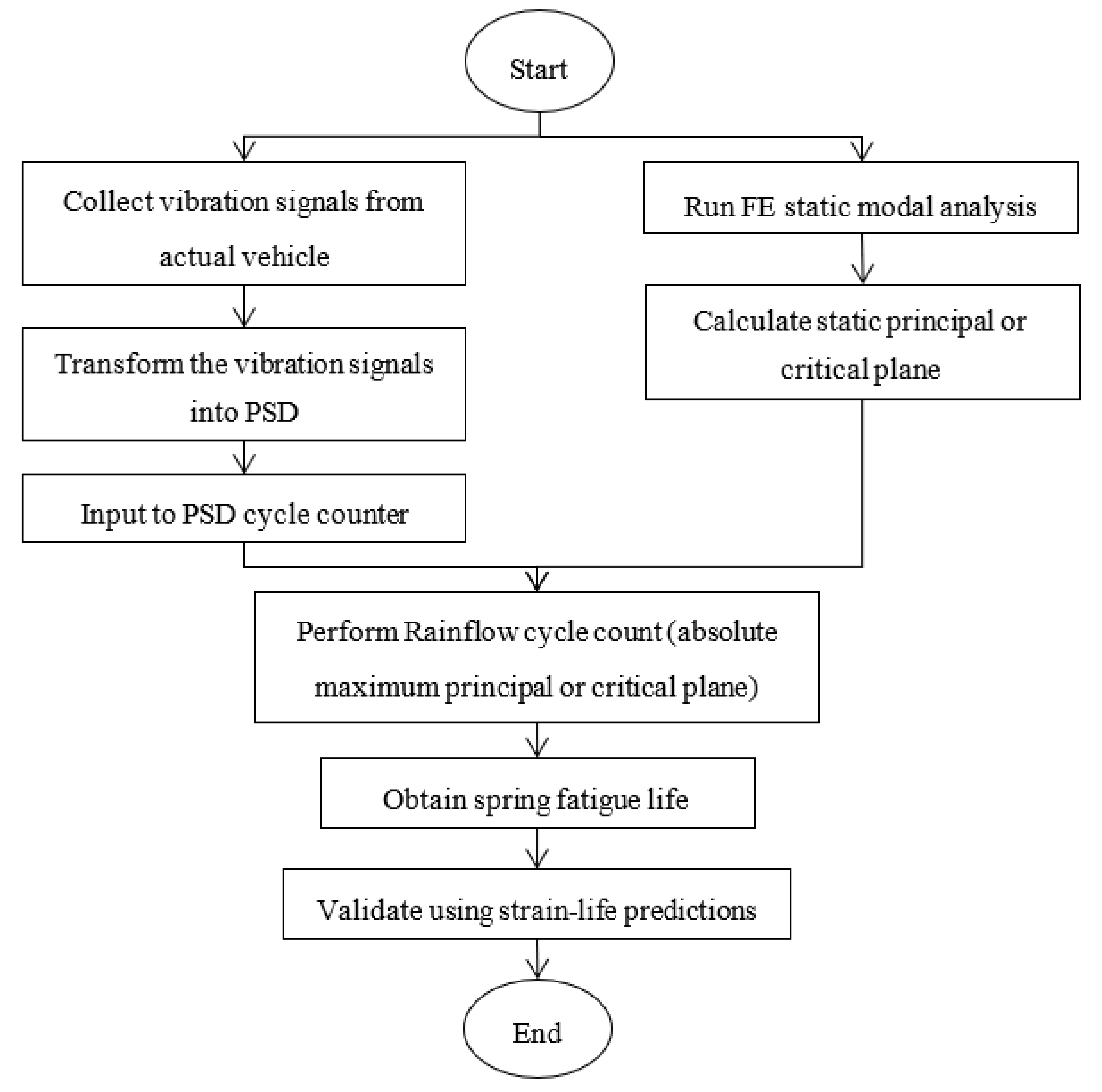
In this analysis, a frontal coil spring of local automobile was used as the case study. The material for the coil spring was SAE 5160 carbon steel where this material was widely used as the spring material. The required material cyclic properties for this carbon steel are listed in

Table 1. Mechanical properties of the carbon steel [27].

Parameters	Value
Yield strength (MPa)	1487
Ultimate tensile strength (MPa)	1584
Elastic modulus (GPa)	207
Standard error of log(N)	0

. Meanwhile, the chemical composition and cyclic properties of the material are shown in

Table 2. Chemical composition of the carbon steel [27].

Carbon	Silicon	Manganese	Chrome	Molybdenum	Vanadium
0.56–0.64%	0.15–0.3%	0.75–1%	0.7–0.9%	0.15–0.25%	0.15%

and

Table 3. Cyclic properties of the carbon steel [27].

Properties	Values
Fatigue strength coefficient (MPa)	2063
Fatigue strength exponent	−0.08
Fatigue ductility exponent	−1.05
Fatigue ductility coefficient	9.56
Cyclic strain hardening exponent	0.05
Cyclic strength coefficient (MPa)	1940
Poisson ratio	0.27

, respectively. Based on the carbon content, this type of steel is classified as medium carbon steel. The process flow for the fatigue life assessment of the coil spring is shown in Figure 1. Initially, the geometry of the coil spring was obtained and pre-processed using three-dimensional (3D) solid hexahedron elements. A total of 9227 nodes and 7170 elements were obtained for this spring model. In order to identify the normal mode of the coil spring, FE modal analysis was performed using the Lanczos method [26]. One end of the coil spring was fixed with a rigid body and fixed boundary conditions to ensure that there was no movement allowed. This kind of modal analysis configuration was known as a “fixed-free” setting where boundary conditions were applied.

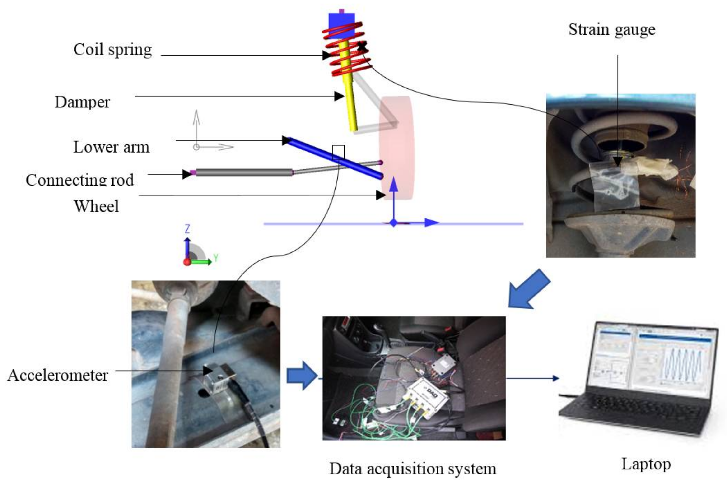
For loading signals collection, the vibration time histories were collected using an uni-axis accelerometer that was attached at the lower arm of the automobile which was close to the coil spring as shown in Figure 2. In addition, a strain gauge was also applied at the critical point of coil spring for strain data measurement. The passenger car was then drive through different road for acceleration signals collection where the road could be classified into highway, rural area, and residential road. A sampling rate of 1000 Hz was determined during the data collection process to ensure that all of the required information was captured [28]. For signal processing, the collected acceleration signals in forms of VAL were then transformed into PSD for frequency domain vibration fatigue analysis. The PSD were used as input to the PSD cycle counter, like Lalanne, Dirlik, narrow band approaches.

For structural dynamics, the eigenvalues and eigenfrequencies were calculated in order to determine the natural frequencies and mode of the coil spring using Lanczos eigensolver. After identified the corresponding mode shapes and natural frequencies, the frequency response function (FRF) analysis of the coil spring was conducted. A dummy 1 g acceleration loading was applied at another end of the coil spring in order to determine the modal stress of the component because this magnitude was further used as the scale factor with measured acceleration for vibration fatigue analysis. For fatigue analysis, a single PSD was used for each node showing some stress invariant, like absolute maximum principal and critical plane stress. These are obtained by taking the eigenvalues of the stress tensor matrix, as follows [24]:

$$\left[\begin{array}{c}{\sigma }_1\left(\omega \right)\\ {\sigma }_2\left(\omega \right)\\ {\sigma }_3\left(\omega \right)\end{array}\right]=eigenvalues\left\{\left[\begin{array}{ccc}{S}_{xx}\left(\omega \right)& S_{xy}\left(\omega \right)& S_{xz}\left(\omega \right)\\ S_{xy}\left(\omega \right)& S_{yy}\left(\omega \right)& S_{yz}\left(\omega \right)\\ S_{xz}\left(\omega \right)& S_{yz}\left(\omega \right)& S_{zz}\left(\omega \right)\end{array}\right]\right\}$$

(20)

When using the absolute maximum principal approach, the predicted local stress response, G_abs(f) was obtained, as follows [24]:

$$G_{abs}\left(f\right)=P\left(f\right)·{\left|X_{abs}\left(f\right)\right|}^2$$

(21)

where P(f) is the PSD loading and X_abs(f) is the FRF of absolute maximum principal stress. For the case of critical plane, the local stress response G_Ø(f) was obtained, as follows [24]:

$$G_{Ø}\left(f\right)=P\left(f\right)·{\left|X_{Ø}\left(f\right)\right|}^2$$

(22)

where X_Ø(f) is the FRF for critical plane approach. Then, the fatigue life was obtained using through the standard stress-life (S-N) approach with the nCode^® Designlife^® setup, as shown in Figure 3. For validations, the collected strain data was processed using material cyclic properties and Coffin-Manson strain life approach to obtain the fatigue life. Coffin-Manson relationship was selected because this approach did not consider the mean stress effects, which is the same to vibration fatigue analysis. Then, both the predicted fatigue lives were correlated using a 1:2 or 2:1 fatigue approach to determine the accuracy of predictions.

4. Results and Discussion

To predict the fatigue life in frequency domain, the acceleration loading signals from different road conditions were acquired. The acceleration loading signals were collected from the lower arm of a passenger car that was driven across different terrain, as shown in Figure 4, while the simultaneously collected strain signals are shown in Figure 5. In Figure 4 and Figure 5, the road conditions were classified into highway, residential, and rural road where the surface roughness of each road was varying. Hence, to characterise the road acceleration measurement, the statistical parameter, like mean, r.m.s, and kurtosis were used to analyse the data characteristic, as shown in Table 1. These four parameters were significant for fatigue life predictions using acceleration signals because the analyses were always depending on the occurrence of peaks and mean value.

As observed from

Table 4. Statistical analysis of acceleration signals.

	Highway	Residential	Rural
Mean (m/s2)	0.0064	0.0045	0.0442
r.m.s (m/s2)	0.2664	0.1584	1.2479
Kurtosis (m/s2)	4.0169	4.8416	4.4625

, the mean value of the acceleration signals was low for all three road conditions. This was because the vibration of the vehicle was usually occurred equally at a fixed position. To investigate the vibration energy of the acceleration signal, the root mean square (r.m.s) was analysed. It was found that the rural road acceleration signal consisted of the highest r.m.s value, which also indicates the highest vibration energy [29]. The residential road acceleration had the highest kurtosis value above three, which shows that the signals were heavily non-stationary and with mesokurtic data distribution [1]. Kurtosis and r.m.s values tended to affect the fatigue life of the components where a high r.m.s value induced high fatigue damage to the coil spring. Meanwhile, the same statistical parameters were also applied on strain measurement, as listed in

Table 5. Statistical analysis of strain signals.

	Highway	Residential	Rural
Mean (µε)	0.0095	0.0045	0.0442
r.m.s (µε)	210.95	509.26	748.91
Kurtosis (µε)	3.3168	4.3518	5.7322

. The strain signals have also revealed a low mean value, but the trend of r.m.s was the same as the acceleration signals, which meant that the strain signals had equivalent information of road excitations with the acceleration signals.

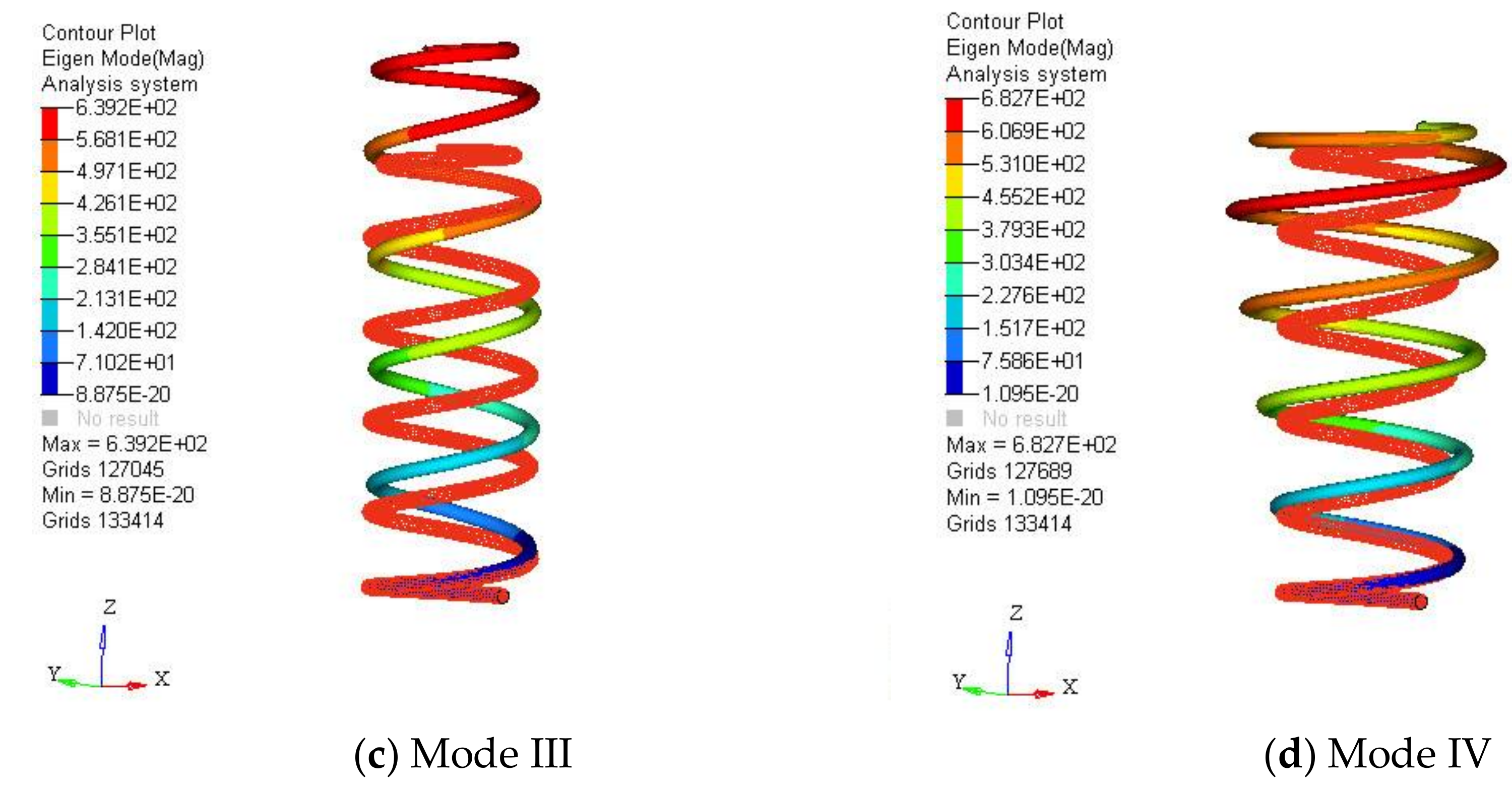
When the vibration loadings that were induced from road profiles resonated with the coil spring, extra displacement was induced on the spring and led to additional fatigue damage. Hence, to estimate the resonance frequency of the spring structure, modal FRF of the fixed-free coil spring was performed and the results are shown in Figure 6. In Figure 6, first four mode shapes of coil spring with natural frequencies were presented. As observed, Mode I and Mode II were the lateral mode of the coil in X and Y axis, while the Mode III was the axial mode of the spring. Meanwhile, Mode IV was the extension mode of the spring. Sun et al. [30] reported the equivalent first four mode shapes for a coil spring. In this analysis, the Mode I and II possessed natural frequencies of 173 and 180 Hz. Mode III was the critical mode where the spring was designed to operate in vertical Z-axis and it had a frequency of 458 Hz. Meanwhile, the extension mode had high frequency of 550 Hz. When the frequency of road induced acceleration loadings matched with these natural frequencies, the spring was resonated, and fatigue damage accumulated until fatigue failure occurred. However, the PSD of the measured acceleration signals were only up to 500 Hz where it considered only the first three modes of the spring modal analysis during fatigue life predictions.

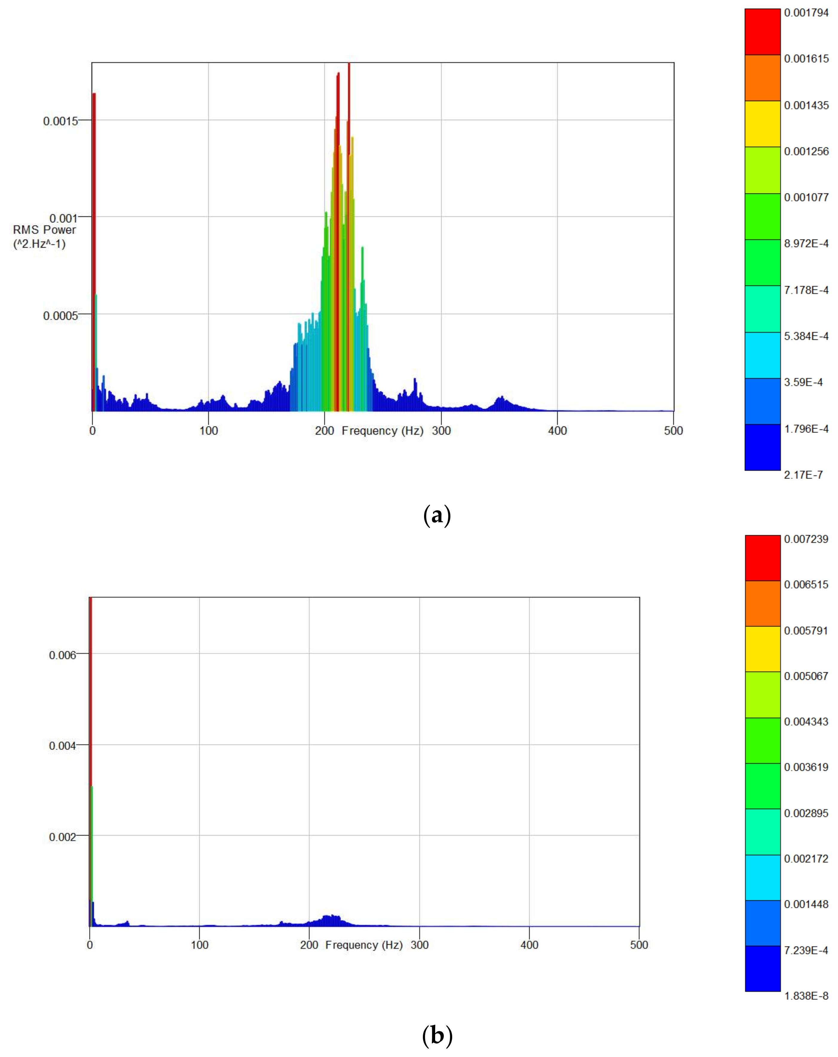
To assess the fatigue life of the coil spring using frequency domain approach, the acquired acceleration signals were transformed into power spectra density (PSD) to determine the energy of each frequency range. The PSD for all three road conditions were obtained, as shown in Figure 7. As observed from Figure 7, the peaks of PSD were occurred at two frequency range, which were from 0 to 20 Hz and 180 to 220 Hz. The high frequency peaks at 210 Hz were due to the vibrations that were induced by engine and transmission system [31]. For the highway road, the peak amplitude for road and transmission induced vibrations consisted of similar amplitude around 0.0018 (m/s²)²/Hz. Subsequently, the residential road acceleration had shown a critical peak as high as 0.0072 (m/s²)²/Hz at low frequency range because the residential road consisted of many speed bumps, which caused the high amplitude peaks. Nevertheless, the peaks were also observed at rural area road due to potholes that caused peaks as high as 0.5074 (m/s²)²/Hz at low frequency. The high peaks for all of the roads were expected to cause high fatigue damage to the spring.

After the PSDs were obtained, the PSD cycle counters were applied to find equivalent decomposed simple reversal cycles. The acceleration reversal cycle count of all three road conditions using Lalanne method is shown in Figure 8. Lalanne assumed that, over a sufficient long time, the probability density function (PDF) of peaks were in the simple weighted sum of Rayleigh and Gaussian distributions [14]. For the highway road case, the maximum range was 4.2118 m/s² where these amplitudes appeared 4.82 × 10⁻¹⁰ cycles. For the residential area, the maximum range was 4.8491 m/s² where the amplitudes appeared 4.85 × 10⁻¹⁰ cycles. Thirdly, the maximum range for rural road was 18.8483 m/s² with 1.72 × 10⁻¹⁰ cycles. These counted cycles were obtained as equivalent Rainflow decomposed simple reversal cycle from PSD where these amplitudes directly contributed to the fatigue damage.

The concept of the Dirlik method was different from Lalanne where it proposed that the PDF of peaks were a combination of an exponential and two Rayleigh densities [24]. Hence, it possessed different distribution when compared to the Lalanne PSD cycle counter, as shown in Figure 9. As observed from Figure 9, the shape of the cycle distribution decayed faster than the Lalanne approach because of the integrated exponential distribution function. In addition, the Dirlik distributions of low amplitude were more frequent than the Lalanne cycle counter. Meanwhile, the narrow band PSD cycle counter method is shown in Figure 10. This narrow band PSD cycle counting considered the amplitude distribution in Rayleigh form. When the narrow band method applied to wide band processes, it tended to overestimate the Rainflow fatigue damage [32]. For all three PSD cycle count method, the maximum range of peaks was equivalent, but the frequencies of the small amplitude were varying. When the number of peaks was different, it led to different fatigue damage, and subsequently affecting the total fatigue life.

After the PSD cycle counting, the results were implemented to obtain the spring fatigue life. The stress responses were obtained through integrating the PSD cycle count amplitude with the spring FEA modal analysis. Then, the fatigue life was calculated using stress-life (S-N) curve when the stress responses were obtained. The fatigue life and damage contour plot of spring using the Lalanne PSD cycle count and the absolute maximum principal stress criterion under different road conditions is shown in Figure 11 and Figure 12, respectively. Based on the fatigue damage contour, the spring experienced higher damage at the inner surface. As a support, Llano-Vizcaya [32] reported the same high stress region of a coil spring using FEA. In this case, the highway road produced lesser fatigue damage to the spring, and hence higher fatigue life was obtained. The second-high fatigue damage contributor was the residential road. For the most critical case, the rural road consisted of several potholes, which caused extra deformation on the spring has led to the highest fatigue damage among three road conditions.

In this analysis, various stress criterions with PSD cycle counter were applied to determine their effects on spring fatigue life. The results of spring fatigue life under highway road excitations and absolute maximum principal stress criterion were listed in

Table 6. Fatigue life using absolute maximum principal stress under highway road excitation.

PSD Cycle Counter	Fatigue Damage	Largest Stress Cycle Amplitude (MPa)	Fatigue Life (Blocks to Failure)
Lalanne	3.65 × 10−18	176.6	2.74 × 1017
Dirlik	1.94 × 10−18	176.6	5.16 × 1017
Narrow band	1.44 × 10−17	176.6	7.11 × 1016

. Based on the results, the fatigue lives of spring using Lalanne and Dirlik PSD cycle counter under highway road excitations were 2.76 × 10¹⁷ and 5.21 × 10¹⁷ blocks to failure, which were higher than the narrow band approach prediction of 7.17 × 10¹⁶ blocks to failure. This was due to the narrow band method being conservative when dealing with the wide-band process [33]. However, based on the observation on PSD, the acceleration band was sharp and narrow, which was mostly narrow band but highway road signals possessed a wide band at frequency 210 Hz. For the largest stress cycle amplitude of the highway, the maximum stress value was 176.6 MPa. This stress level was much lower than the material’s yield strength of 1487 MPa, which indicates that this design of spring was safe under static loading.

For critical plane approach, the largest stress cycle amplitude was 176.2 MPa, which was slightly lower than absolute maximum principal stress criterion. Using this stress amplitude, the fatigue life was predicted using the critical plane approach, as listed in

Table 7. Fatigue life using critical plane approach under highway road excitation.

PSD Cycle Counter	Fatigue Damage	Largest Stress Cycle Amplitude (MPa)	Fatigue Life (Blocks to Failure)
Lalanne	3.62 × 10−18	176.2	2.76 × 1017
Dirlik	1.92 × 10−18	176.2	5.21 × 1017
Narrow band	1.40 × 10−17	176.2	7.17 × 1016

. Since the cycle amplitude was reduced, the accumulated fatigue damage was also reduced, and hence, higher fatigue life was obtained. When investigated the residential road frequency-based predicted fatigue life, the largest stress cycle amplitude has been increased to 237.7 MPa, as shown in

Table 8. Fatigue life using absolute maximum principal stress under residential road excitation.

PSD Cycle Counter	Fatigue Damage	Largest Stress Cycle Amplitude (MPa)	Fatigue Life (Blocks to Failure)
Lalanne	4.47 × 10−12	237.7	2.24 × 1011
Dirlik	1.55 × 10−12	237.7	6.46 × 1011
Narrow band	2.25 × 10−11	237.7	4.44 × 1010

. When compared to the highway road, the stress cycle was higher and hence it yielded larger fatigue damage. Subsequently, the critical plane approach was also analysed in order to determine the fatigue life as listed in

Table 9. Fatigue life using critical plane approach under residential road excitation.

PSD Cycle Counter	Fatigue Damage	Largest Stress Cycle Amplitude (MPa)	Fatigue Life (Blocks to Failure)
Lalanne	4.43 × 10−12	237.3	2.26 × 1011
Dirlik	1.53 × 10−12	237.3	6.52 × 1011
Narrow band	2.23 × 10−11	237.3	4.48 × 1010

. In this case, the largest stress cycle was also lower than the absolute maximum principal stress approach, which was 237.3 MPa. Hence, the predicted fatigue life was also lower than the absolute maximum principal stress results.

Thirdly, the fatigue lives of spring under rural road excitations were investigated using absolute maximum principal stress, as shown in

Table 10. Fatigue life using absolute maximum principal stress under rural road excitation.

PSD Cycle Counter	Fatigue Damage	Largest Stress Cycle Amplitude (MPa)	Fatigue Life (Blocks to Failure)
Lalanne	5.44 × 10−8	370.2	1.84 × 107
Dirlik	2.28 × 10−8	370.2	4.38 × 107
Narrow band	1.77 × 10−7	370.2	5.64 × 106

. As observed from statistical parameters, the rural area acceleration signal had the highest r.m.s value, and hence possessed the highest vibration energy. The rough rural roads induced more vibration to the suspension system and more deformation on the spring which also lead to higher strain value. Meanwhile, the largest stress cycle for this rural area road excitation was 370.2 MPa which was also higher when compared to the highway and residential road excitations. Apparently, this parameter led also to the highest fatigue damage and lower fatigue life when compared to the prediction results under highway and residential road accelerations. In

Table 11. Fatigue life using critical plane approach under rural road excitation.

PSD Cycle Counter	Fatigue Damage	Largest Stress Cycle Amplitude (MPa)	Fatigue Life (Blocks to Failure)
Lalanne	5.39 × 10−8	369.6	1.86 × 107
Dirlik	2.26 × 10−8	369.6	4.42 × 107
Narrow band	1.76 × 10−7	369.6	5.69 × 106

, the critical plane analysis of rural road acceleration signals was performed where the largest stress cycle amplitude was 369.6 MPa. The peak stress was slightly lower than the absolute maximum principal stress approach where the obtained fatigue life was slightly higher. Under the most critical rural road influence, the required time to fatigue failure was about 150 years, which indicates that the spring has an extreme long of service life.

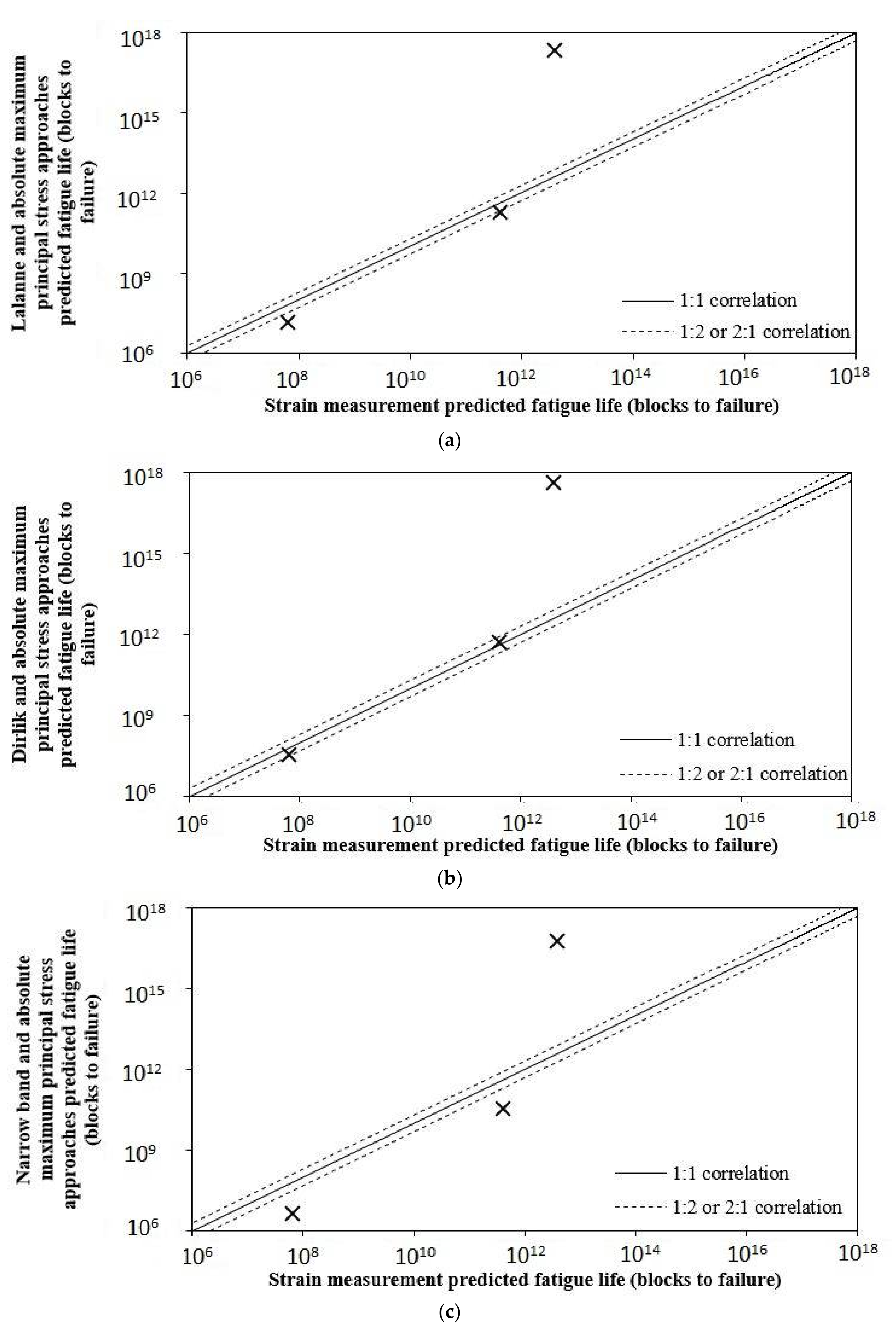
Prediction of fatigue life using strain time histories was one of the most acceptable approaches [34]. To show the correlation of vibration fatigue prediction according to the strain-life approaches, the strain signals were applied to the Coffin-Manson strain-life model for fatigue life analysis. In accordance with that, the obtained results are tabulated into

Table 12. Strain predicted fatigue life using Coffin-Manson relationship.

Road Conditions	Fatigue Life (Blocks to Failure)
Highway	3.52 × 1011
Residential	3.73 × 1010
Rural	5.71 × 107

. Coffin-Manson strain-life approach was selected because mean stress was absent in both approaches [35]. Based on the strain predicted results, the rural road possessed the lowest fatigue life, followed by the residential and highway road. This trend of fatigue life was close to the vibration predictions. To further investigate the vibration predictions, the vibration predicted fatigue lives were plotted against the strain predicted fatigue life using a 1:2 or 2:1 conservation fatigue correlation curve, as shown in Figure 13 and Figure 14.

When a fatigue life lied within the 1:2 or 2:1 boundary, the predicted fatigue life was considered to have a good correlation with the predictor [36]. Based on the correlation curve from Figure 13a, two out of three Lalanne PSD cycle counter and absolute maximum principal predicted fatigue lives lay beyond the 1:2 or 2:1 region. The highway fatigue life lay far beyond the acceptable region because the collected acceleration signals were very small and far beyond the endurance limit. For the Dirlik approach, the rural and residential road predicted fatigue lives were lay within the acceptable region. Nevertheless, the fatigue life under highway road was also beyond the acceptable region. For the non-conservative case, the narrow band predicted fatigue lives all fall beyond the boundary. This indicating the narrow band cycle counter was not good in predicting the fatigue life, while the Dirlik approach has shown a better performance than other approaches.

The critical plane approach was also correlated to the strain predicted fatigue life, as shown in Figure 14. The fatigue life prediction results of critical plane have the same trend with absolute maximum principal approach, but with a lower value. The critical plane approach determined the plane with the maximised stress state where the shear stresses were considered, and this method provided smaller fatigue scatter error [16]. For fatigue assessment, the critical part was the coherency of the solutions where it was possible to obtain the same results by using any approaches. In this analysis, fatigue assessment of automobile coil spring was performed using frequency domain and it correlated with the strain-life time domain approach where a good correlation was obtained. The significance of frequency domain approach is the flexibility where the same signals could be used for other components [37].

The prediction of fatigue life in frequency domain has drastically reduced the computing time due to integral convolution [3]. The strain-life approach utilised the long strain time history to predict fatigue life, while the frequency domain transformed the long loading time histories into PSD for fatigue life predictions. Regardless, how long was the sampling time, frequency approach maintained the PSD range but with varying peaks. Therefore, the frequency domain was more efficient in computing the fatigue life because less data points were required. On the other hand, when dealing with a dynamic component, the influence of each mode in a dynamic response was important. The mode shapes and frequencies represented the dynamical behaviour of the coil spring where the excitation of loadings on individual mode shapes was identified. When the load frequencies were close to the system resonant frequencies, the stronger the dynamic response.

Another significant contribution of this research works was using the modal analysis approach to assist the spring design in terms of fatigue life. When the spring design suffered from a lower fatigue life, a new spring design to strengthen the fatigue life was required. In this case, the spring design was analysed using modal analysis to avoid the matching of the loading excitations, which reduced the fatigue life due to resonances. In this analysis, the loading definition for fatigue life prediction in frequency domain was acceleration. This was a critical part of using this frequency domain fatigue assessment. The measured acceleration signals could be used to assess fatigue damage for different structural components of a vehicle according to the durability transfer concept. Hence, the impractical strain measurement on every critical component of the vehicle was reduced, which inferred that the fatigue assessment of components using acceleration signals were pragmatic.

5. Conclusions

As for conclusion, fatigue life predictions of automobile coil spring have been successfully predicted using the frequency-based fatigue approach. The fatigue life was well-correlated to the Coffin-Manson strain life approach using scatter band method. Dirlik frequency approach has shown the closest predictions to the Coffin-Manson strain life predicted results. Under the harshest rural road conditions, the spring has a fatigue life of 4.47 × 10⁷ blocks to failure, which is equivalent to a lifetime of 153 years. This suggested that the spring design was good to deal with the harsh road conditions without premature failure. In this new trend of automotive industry, the spring design is needed to be optimised for material reduction, while maintaining the required fatigue life where the outcome of this research could contribute to the spring design processes.

References

- Teixeira, G.M.; Jones, D.; Draper, J. Random Vibration Fatigue—A Study Comparing Time Domain and Frequency Domain Approaches for Automotive Applications; SAE Technical Paper; SAE: Warrendale, PA, USA, 2014. [Google Scholar]
- Jadav Chetan, S.; Panchal Khushbu, C.; Fajalhusen, P. A review of the fatigue analysis of an automobile frames. Int. J. Adv. Comput. Res. 2012, 2, 103–107. [Google Scholar]
- Herve, R.; Mohamed, B.; Tony, D.S.; Fabien, L. Comparison of spectral methods for fatigue analysis in non-Gaussian random processes—Application to elastic-plastic behaviour. Procedia Eng. 2015, 101, 430–439. [Google Scholar] [CrossRef]
- Wang, L.; Burger, R.; Aloe, A. Considerations of vibration fatigue for automotive components. SAE Int. J. Commer. Veh. 2017, 10, 150–158. [Google Scholar] [CrossRef]
- Kagnici, F. Vibration induced fatigue assessment in vehicle development process. Int. J. Mech. Mechatron. Eng. 2012, 6, 750–755. [Google Scholar]
- Moon, S.I.; Cho, I.J.; Yoon, D. Fatigue life evaluation of mechanical components using vibration fatigue analysis technique. J. Mech. Sci. Technol. 2011, 25, 631–637. [Google Scholar] [CrossRef]
- Palmieri, M.; Česnik, M.; Slavič, J.; Cianetti, F.; Boltežar, M. Non-Gaussianity and non-stationary in vibration fatigue. Int. J. Fatigue 2017, 97, 9–19. [Google Scholar] [CrossRef]
- Kong, Y.S.; Omar, M.Z.; Chua, L.B.; Abdullah, S. Fatigue life prediction of parabolic leaf spring under various road conditions. Eng. Fail. Anal. 2014, 46, 92–103. [Google Scholar] [CrossRef]
- Han, S.G.; An, D.G.; Kwak, S.J.; Kang, K.W. Vibration fatigue analysis for multi-point spot-welded joints based on frequency response changes due to fatigue damage accumulation. Int. J. Fatigue 2013, 48, 170–177. [Google Scholar] [CrossRef]
- Haiba, M.; Barton, D.C.; Brooks, P.C.; Levesley, M.C. Review of life assessment techniques applied to dynamically loaded automotive components. Comput. Struct. 2002, 80, 481–494. [Google Scholar] [CrossRef]
- Kang, B.J.; Sin, H.C.; Kim, J.H.; Kang, H.C. Optimal shape design of the front wheel lower control arm considering dynamic effects. Int. J. Automot. Technol. 2007, 8, 309–317. [Google Scholar]
- Stenti, A.; Moens, D.; Sas, P.; Desmet, W. Low-frequency dynamic analysis of automotive door weather-strip seals. Mech. Syst. Signal Process. 2008, 22, 1248–1260. [Google Scholar] [CrossRef]
- Sani, M.S.M.; Noor, M.M.; Zainury, M.S.M.; Rejab, M.R.M.; Kadirgama, K.; Rahman, M.M. Investigation on modal transient response analysis of engine crankshaft structure. High Perform. Struct. Mater. V 2010, 112, 419–428. [Google Scholar] [Green Version]
- Huang, J.; Krousgrill, C.M.; Bajaj, A.K. Modeling of automotive drum brakes for squeal and parameter sensitivity analysis. J. Sound Vib. 2006, 289, 245–263. [Google Scholar] [CrossRef]
- Klis, R.; Chatzi, E.; Asce, A.M.; Galliot, C.; Luchsinger, R.; Feltrin, G.M. Modal identification and dynamic response assessment of a tensairity girder. J. Struct. Eng. 2017, 143, 03016165. [Google Scholar] [CrossRef]
- Rajappan, R.; Vivekanandhan, M. Static and modal analysis of chassis by using FEA. Int. J. Eng. 2013, 2, 63–73. [Google Scholar]
- Kong, Y.S.; Omar, M.Z.; Chua, L.B.; Abdullah, S. Ride quality assessment of bus suspension system through modal frequency response approach. Adv. Mech. Eng. 2014, 269721. [Google Scholar] [CrossRef]
- Lin, J.; Li, W.; Yang, S.; Zhang, J. Vibration fatigue damage accumulation of Ti-6Al-4V under constant and sequenced variable loading conditions. Metals 2018, 8, 296. [Google Scholar] [CrossRef]
- Mehdi Mahmoodi, K.; Davoodabadi, I.; Višnjić, V.; Afkar, A. Stress and dynamic analysis of optimized trailer chassis. Tehnički Vjesnik 2014, 21, 599–608. [Google Scholar]
- Mršnik, M.; Slavič, J.; Boltežar, M. Vibration fatigue using modal decomposition. Mech. Syst. Signal Process. 2018, 98, 548–556. [Google Scholar] [CrossRef]
- Quigley, J.P.; Lee, Y.L.; Wang, L. Review and assessment of frequency-based fatigue damage models. SAE Int. J. Mater. Manuf. 2016, 9, 565–577. [Google Scholar] [CrossRef]
- Qiang, R.; Wang, H. Frequency domain fatigue assessment of vehicle component under random load spectrum. J. Phys. 2011, 305, 012060. [Google Scholar] [CrossRef]
- Datta, S.; Bishop, N.; Atkins, A. Simultaneous Durability Assessment and Relative Random Analysis under Base Shake Loading Conditions; SAE Technical Paper; SAE: Warrendale, PA, USA, 2017. [Google Scholar]
- Benasciutti, D.; Tovo, R. Spectral methods for lifetime prediction under wide-band stationary random processes. Int. J. Fatigue 2005, 27, 867–877. [Google Scholar] [CrossRef]
- Engin, Z.; Coker, D. Comparison of equivalent stress methods with critical plane approaches for multiaxial high cycle fatigue assessment. Procedia Struct. Integr. 2017, 5, 1229–1236. [Google Scholar] [CrossRef]
- Gawryluk, J.; Bocheński, M.; Teter, A. Modal analysis of laminated “CAS” and “CUS” box-beams. Arch. Mech. Eng. 2017, 64, 441–454. [Google Scholar] [CrossRef]
- Gonzales, M.A.C.; Barrios, D.B.; de Lima, N.B.; Goncalves, E. Importance of considering a material micro-failure criterion in the numerical modelling of the shot peening process applied to parabolic leaf spring. Lat. Am. J. Solids Struct. 2010, 7, 21–40. [Google Scholar]
- Kong, Y.S.; Abdullah, S.; Schramm, D.; Omar, M.Z.; Haris, S.M. Mission profiling of road data measurement for coil spring fatigue life. Measurement 2017, 107, 99–110. [Google Scholar] [CrossRef]
- Igba, J.; Alemzadeh, K.; Durugbo, C.; Eiriksson, E.T. Analysing RMS and peak values of vibration signals for condition monitoring of wind turbine gearboxes. Renew. Energy 2016, 91, 90–106. [Google Scholar] [CrossRef]
- Sun, W.; Thompson, D.J.; Zhou, J.; Gong, D. Analysis of dynamic stiffness effect of primary suspension helical springs on railway vehicle vibration. J. Phys. 2016, 744, 012149. [Google Scholar] [CrossRef]
- Li, C.; Kim, Y.I.; Jeswiet, J. Conceptual and detailed design of an automotive engine cradle by using topology, shape, and size optimization. Struct. Multidiscip. Optim. 2015, 51, 547–564. [Google Scholar] [CrossRef]
- Llano-Vizcaya, L.D.; Rubio-González, G.; Cervantes-Hernández, T. Multiaxial fatigue and failure analysis of helical compression springs. Eng. Fail. Anal. 2006, 13, 1303–1313. [Google Scholar] [CrossRef]
- Rychlik, I. On the “narrow-band” approximation for expected fatigue damage. Probab. Eng. Mech. 1993, 8, 1–4. [Google Scholar] [CrossRef]
- Baek, S.H.; Cho, S.S.; Joo, W.S. Fatigue life prediction based on the Rainflow cycle counting method for the end beam of a freight car bogie. Int. J. Automot. Technol. 2008, 9, 95–101. [Google Scholar] [CrossRef]
- Yuan, X.; Yu, W.; Fu, S.; Yu, D.; Chen, X. Effect of mean stress and ratcheting strain on the low cycle fatigue behaviour of a wrought 316LN strainless steel. Mater. Sci. Eng. A 2016, 677, 193–202. [Google Scholar] [CrossRef]
- Mahmud, M.; Abdullah, S.; Ariffin, A.K.; Nopiah, Z.M. Probabilistic scatter band with error distribution for fatigue life comparisons. Exp. Tech. 2017, 41, 505–515. [Google Scholar] [CrossRef]
- Halfpenny, A.; Hussain, S.; McDougall, S.; Pompetzki, M. Investigation of the durability transfer concept for vehicle prognostic applications. In Proceedings of the 2010 NDIA Ground Vehicle Systems Engineering and Technology Symposium, Dearborn, MI, USA, 18 August 2010. [Google Scholar]
Figure 1.
Process flow for coil spring vibration fatigue analysis.
Figure 2.
Experimental setup for strain and acceleration measurements.
Figure 3.
Vibration fatigue analysis using nCode® Designlife®.
Figure 4.
Measured acceleration time histories from different road conditions: (a) highway; (b) residential; and, (c) rural.
Figure 5.
Measured strain time histories from different road conditions: (a) highway; (b) residential; and, (c) rural.
Figure 6.
Mode shape of coil spring for different frequencies: (a) 173 Hz; (b) 180 Hz; (c) 458 Hz; and, (d) 550 Hz.
Figure 7.
Power spectra density (PSD) of acceleration signals for different roads: (a) highway; (b) residential; and, (c) rural.
Figure 8.
Lalanne PSD cycle count for different roads: (a) highway; (b) residential; and, (c) rural.
Figure 9.
Dirlik PSD cycle count for different roads: (a) highway; (b) residential; and, (c) rural.
Figure 10.
Narrow band PSD cycle count for different roads: (a) highway; (b) residential; and, (c) rural.
Figure 11.
Fatigue life contour plot of spring using Lalanne PSD cycle count and absolute maximum principal stress under different roads: (a) highway; (b) residential; and, (c) rural.
Figure 12.
Fatigue damage contour plot of spring using Lalanne PSD cycle count and absolute maximum principal stress under different roads: (a) highway; (b) residential; and, (c) rural.
Figure 13.
Fatigue life correlation curve using absolute maximum principal stress for different PSD cycle counter method: (a) Lalanne; (b) Dirlik; and, (c) Narrow band.
Figure 14.
Fatigue life correlation curve using critical plane stress for different PSD cycle counter method: (a) Lalanne; (b) Dirlik; and, (c) Narrow band.