Using Genetic Algorithms with Multi-Objective Optimization to Adjust Finite Element Models of Welded Joints

Abstract

To ensure realistic results when modeling welded joints using the finite element method (FEM), it is essential to appropriately characterize the thermo-mechanical behavior of the elastic-plastic Finite Element (FE) models. This task is complex. Any small differences between the actual welded joints and the welded joints based on FEM can be amplified enormously in the presence of nonlinearities. Due to the intense concentration of heat on a small area to create such joints, the regions near the weld line undergo severe thermal cycles. These generate significant angular distortion due mainly to the residual stresses. This paper proposes a method to determine the parameters that are most appropriate for modeling the Butt joint single V-groove welded joint FE models’ thermo-mechanical behavior that were created by the one-pass Gas Metal Arc Welding (GMAW). The method is based on experimental data, as well as genetic algorithms (GA) with multi-objective functions. As a practical example, the proposed methodology is validated with three different welded joints specimens that are manufactured by different voltages and currents (26 volts and 140 amps, 28 volts and 210 amps, and 35 volts and 260 amps). The electrode orientation, shielding gas flow rate, distance between nozzle and plate, and welding speed were considered to be constant for all of the specimens that were studied, and their values were 80°, 20.0 L/min, 4.0 mm, and 6 mm/s, respectively. The base material was EN 235JR low carbon steel, whereas the weld bead was ER70S-6 for the three specimens that were welded. An agreement between the temperature field and the angular distortion that was obtained by the adjusted FE models and those that were obtained experimentally demonstrates that the proposed methodology may be valid for automatically determining the most appropriate parameters.

1. Introduction

Gas metal arc welding (GMAW) is used widely in the manufacture of mechanical devices and components. Because such junctions are created by the intense application of heat to a small area, areas that are close to the weld are subject to marked thermal cycles. These cycles cause the microstructure and mechanical properties to change. They also create residual stresses that cause angular distortions in the welded joints. How these welds are created, as well as the welding parameters greatly affect the thermal cycles (Macherauch and Kloos [1]). Various factors directly control several of the welding parameters. These factors include the welding machine’s speed, wire feed rate, pre-heating, voltage, current, shielding gas flow rate, and the mixture’s flux proportion. Additional welding process parameters that the welding machine is unable to control include the distance between the nozzle and plate, the thickness of the plate, and the electrode orientation diameter of the wire. The most frequently studied parameters are voltage, current, and speed. They also are the parameters that most affect the GMAW process (Ozcelik and Moore [2]). For decades, the Finite Element Method (FEM) has been used as an alternative in an attempt to reduce the costs during the design phase of mechanical components and mechanical devices. Despite the obvious advantages of using the FEM, there are some disadvantages, such as convergence problems, especially if the FE model includes nonlinearities. Finite Element (FE) models of welded joints should be modeled in three-dimensional (3D) and consider a nonlinear behavior for the material to be welded, for the thermal contacts. The FE models should be able to accurately capture the temperature distribution, residual stress, and deformations. Also, an accurate evaluation of the residual stresses is very important due to their influence on the fatigue behavior of the welded joints [3,4]. Generally, welded joints in FE models require a large number of parameters to be defined correctly. A failure to establish them in a methodical fashion can cause any small differences between the inappropriate parameters and what would have been appropriate parameters to amplify the difference between the FE model’s results and reality. This means that determining the right values of the parameters that define the FE models, although being a complicated task, is absolutely required if the FE results must be as close as possible to reality (Lostado et al. [5]). Thus, various authors have developed complex FE models to study the temperature field and the distortions in welded joints. However, they have not used any methodology to determine the most appropriate parameters to model the thermo-mechanical behavior in welded joints FE models with experimental data. Thus, (Deng and Murakawa [6]) use an FE model to study the temperature field, as well as residual stresses in stainless steel pipe multi-pass welds that were created by Gas Tungsten Arc Welding (GTAW). The heat from the moving arc welding was modeled by an uncoupled thermal-mechanical FE model and the double ellipsoidal distribution that Goldak et al. proposed [7]. Both conduction and convection were considered, as was the temperature-dependent heat transfer coefficient (Brickstad and Josefson [8]). Ericsson and Nylén [9] developed a combination of a robot simulation and FE simulations to optimize the welding process speed in order to minimize angular distortion. In this case, the FE models were validated by the temperature histories of a group of thermocouples and an infrared camera that were located in different points of the parts to be welded. Finally, Attarha and Sattari-Far [10] studied the welding temperature distribution in the Heat-Affected Zone (HAZ) for joints that were similar and dissimilar to thin butt-welded joints that are manufactured in the Gas Tungsten Arc Welding process (GTAW). In this case, the FEM was used to predict the temperature distributions throughout the plates using ABAQUS software, and experimentally validated with thermocouples. The FE models assumed the radiation, conduction, convection, and the double ellipsoidal distribution that were considered to be the input heat flux. More recently, Lostado et al. [11] studied the temperature field and the Residual Stresses with Time-Independent Cyclic Plasticity in ibutt joints with single V-groove Finite Element (FE) models.

Other researchers have based their studies of welded joints with FEM on angular distortion, instead of temperature fields. For instance, Bachorski et al. [12] developed a FE model to predict the distortion during gas metal arc welding (GMAW) using the volume shrinkage approach. This method considered the post-weld distortion and assumed a linear thermal contraction for the FE model. Pilipenko [13] studied by means of FE models the transverse, longitudinal, and angular shrinkage, as well as the bending distortion, in the multi-electrode submerged arc welding process (SAW). In another work, Zhang et al. [14] used a combination of FE models and experiments to investigate the effects of arc distance and welding parameters in controlling residual angular distortion in the Tungsten Inert Gas (TIG) process. The FE models considered temperature-dependent material behavior and double ellipsoidal distribution (Goldak et al. [7]) for the input heat flux. More recent and complete work has included both the temperature field and angular distortion to validate welded joints FE models. For example, Aarbogh et al. [15] modeled the distortion and temperature fields of a single pass metal inert gas welding (MIG) on an austenitic steel plate by means of WeldSimS numerical code (Chao et al. [16]). In this study, the authors considered the coupled thermal-mechanical fields, temperature-dependent material, and the phenomena of conduction, convection, and radiation, for the FE models that they proposed. The heat from the moving welding arc was also modeled assuming a double ellipsoidal distribution. Tian et al. [17] studied a Butt joint with partial penetration groove weld (a single V-groove) that was generated by a Tungsten Gas Arc (GTA). The input parameters that were studied to obtain the temperature field, angular distortion, and transverse shrinkage were voltage, speed, and current. The input parameters and data that were obtained were used to validate a three-dimensional FE model. A T-joint fillet welded joint FE model using simplified material properties was used by Perić et al. [18] to investigate the influence of the temperature-dependent thermo-mechanical material properties of carbon steel. The proposed FE model was validated by means of residual stresses and angular distortions from a series of experiments that involved a fully automated welding process.

The parameters of the welded joints FE models that were adjusted by most of these cited authors are related to the conduction and the convection phenomenon and elastic-plastic material behavior. They made the FE model adjustments without further procedures. They only used the test error method, which has an unacceptable computational cost. This paper proposes a method by which to automate the adjustment of the parameters that define those of welded joint FE models. The proposal is based on experimental data and genetic algorithms (GA) with multi-objective functions. The paper applies the adjustment methodology to butt joint single V-groove welds of EN 235JR low carbon steel that have been produced by a one-pass Gas Metal Arc Welding (GMAW) process. In this case, the effects of phase transformation were not considered because the base material (EN 235JR) had a low carbon content, as did the weld bead (wire ER70S-6), and the slow cooling of all the welded specimens in this study. Three Butt joint single V-groove weld FE models that considered the rate independent plasticity behavior were generated by 13 different parameters. These parameters were considered to define the conduction and convection phenomena, as well as the weld flux. In addition, each of the three welded joint FE models considered different voltages and currents (26 volts and 140 amps, 28 volts and 210 amps, and 35 volts and 260 amps) and a speed of 6 mm/s. The methodology for adjusting such welded joint FE models was validated by three different welded joints specimens that were manufactured with the same voltages and currents (26 volts and 140 amps, 28 volts and 210 amps, and 35 volts and 260 amps). Also, it was assumed that the welding process configuration (electrode orientation, shielding gas flow rate, distance between nozzle and plate, and welding speed) were constant for all of the specimens that were manufactured with 80°, 20.0 L/min, 4.0 mm, and 6 mm/s, respectively. The wire for each study specimen was an ER70S-6 of 1.2 mm diameter and with mechanical behavior and a chemical composition that was similar to that of the base metal. The selection of the ranges for current and voltage, as well as the electrode orientation, shielding gas flow rate, distance between nozzle and plate, and speed at 80°, 20.0 L/min, 4.0 mm, and 6.0 mm/s, respectively, was based on previous studies [19] to avoid defects or complex problems in the welded joint FE models that were studied. These defects are: pores in weld beads, fusion of the plates to be welded, excessively small weld beads that do not completely cover the mechanized zone of the plates, thereby creating the Butt joint single V-groove weld, or excessively large weld beads. However, the adjustment methodology that is proposed in this paper could be applied to adjust the thermo-mechanical behavior of any type of welded joint FE model, while considering such complex effects as phase transformation. In that case, the proposed welded joint FE models would have defined other parameters that are necessary to define the conduction and convection phenomena, as well as the weld flux.

The proposed methodology is as follows. First, a correlation based feature selection (CFS) filter algorithm was applied to each of the three proposed FE welded joints to determine which input parameters most influence the temperature field and angular distortion. The adjustment process using GA to set the parameters of welded FE models that were manufactured with different currents and voltages were developed in two different ways. The first way only considered the most influential parameters that were revealed by CFS. The second way was to consider the totality of the proposed input parameters. An agreement between the temperature field and the angular distortion that were revealed by the proposed FE model and those obtained experimentally demonstrates that the proposed methodology may be valid for determining automatically the most appropriate parameters that are needed to model the thermo-mechanical behavior of welded joint FE models on the basis of experimental data.

2. Determination of the Optimum Material Parameters for the Finite Element Method (FEM) by Genetic Algorithms (GA)

Using GA to adjust FE models is a well-known method that some researchers have used in recent years, especially when these models exhibit highly nonlinear behavior (Lostado et al. [3]; Lostado et al. [20]; Lostado et al. [21]; Gentils et al. [22]; Duanm et al. [23]). In the field of welded joints, some authors (Bag et al. [24]) have used GA to adjust the unknown parameters that define three-dimensional heat transfer FE models when the GTAW process is studied. More recently, other authors, including as Lostado et al. [11], have used GA to adjust the parameters that define the temperature field in butt joints with single V-groove Finite Element (FE) models. In this case, the adjusted parameters were used for FE models in the study of Residual Stresses with Time-Independent Cyclic Plasticity. To date, no further references have been found in the literature that uses GA to adjust FE models or to optimize welding sequences in manufacturing processes in combination with FEM. Other researchers have used the GA to optimize the manufacturing welding sequence on the basis of experimental data without the use of the FEM (Voutchkov et al. [25]; Xie, et al. [26]). In these studies, the optimization process required a significant number of experiments to weld joints in different sequences and with different welding parameters.

3. Genetic Algorithms with Multi-Objective Functions

A population of several individuals is used by Genetic algorithms GA for an optimization that provides a solution that approximates the minimum possible solution. The GA method is applicable to problems like those of biological evolution in a manner that is reminiscent of biological mechanisms (Michalewicz [27]; Fonseca and Fleming [28]). The optimization process using GA is usually conducted by the following six steps: coding/decoding, population initialization, evaluation, selection, crossover, and mutation. To explain the optimization process, assume that we have a mathematical model, or results that were obtained from an experiment f(x₁, …, x_n) and that we wish to find a solution (x₁, …, x_n) that maximizes or minimizes that function or experiments. In the current paper, this function may be the temperature field and the field of angular distortion of the welded joint FE models. First, a basic genetic algorithm creates randomly an initial generation of N individuals. Each solution is encoded in chromosomes and evaluated using, in this case, the FE model G0 (x_k1, …, x_kn) in such a way that the best individuals will be those whose result approaches the desired maximum or minimum result. A new generation is created and evaluated based on the best individuals (those that provide the best solution when the intention is to achieve a single objective, or to achieve several objectives simultaneously). This process is repeated until the best individual in each generation has a value that is close to the desired optimum. Each generation of individuals Gn when n ≠ 0 is usually created from the previous generation. Approximately 25% of new individuals have the best (i.e., the “fittest”, much like the theory of natural selection). A higher percentage of the individuals (e.g., 75%) result from cross-over of chromosomes from the previous generation (sexual reproduction). The remainder (10%) arises from random alteration of selected genes of the previous generation’s chromosomes (mutation). The adjustment process and the proposed methodology for development of the cross-over and mutations for the FE models that are proposed are described in Section 5.2 and Section 5.3.

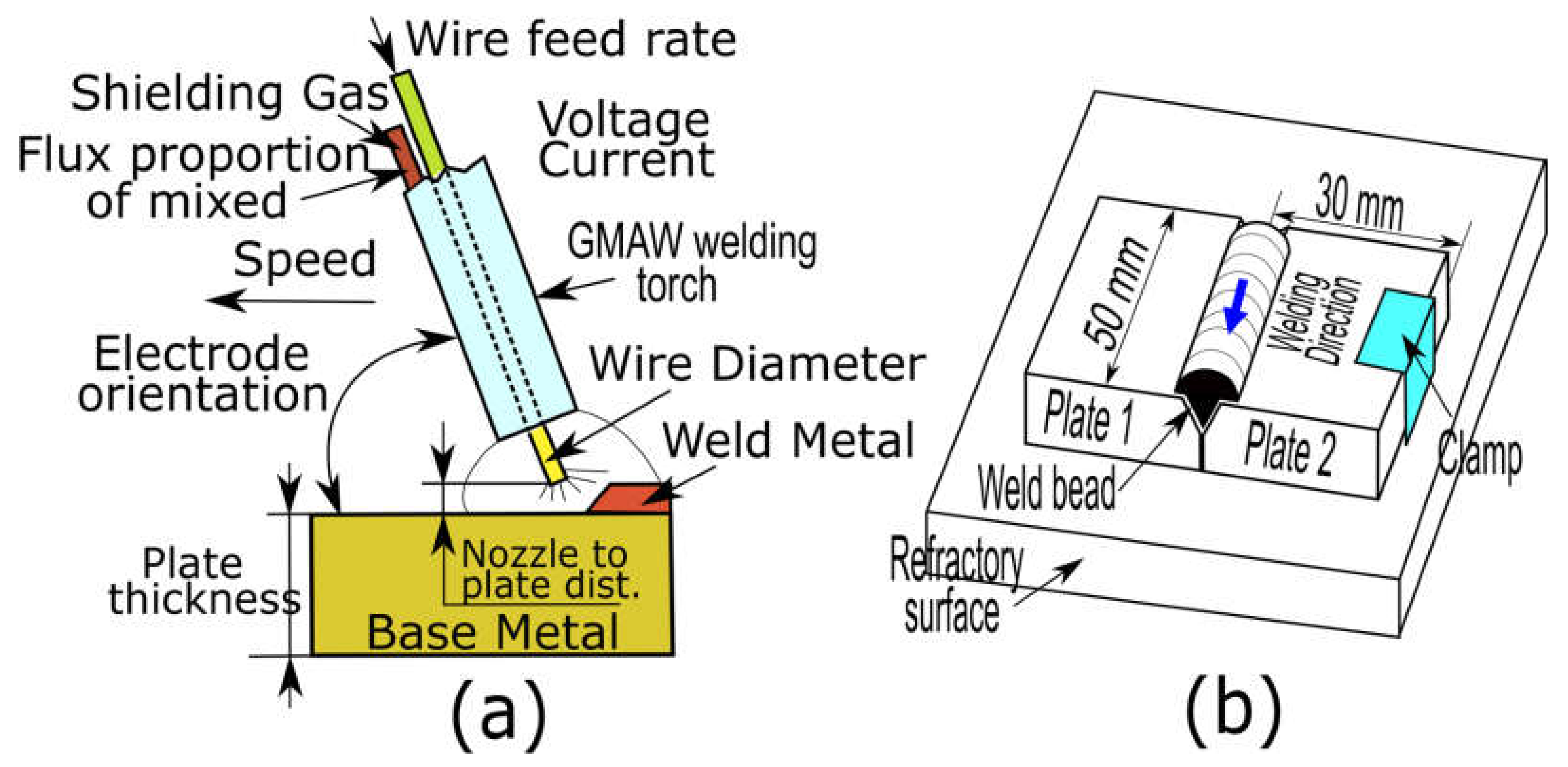
4. Experimental Procedure

The proposed method’s first stage is manufacturing three butt joint specimens that have a single V-groove from EN 235JR low carbon steel and establishing GMAW process configuration parameters. All of the specimens used was ER70S-6 wire of 1.2 mm diameter and are similar to the base metal in mechanical behavior and chemical composition. The specimens were manufactured automatically by an ESAB 180 welding machine into which an ABB 1500 IRB robot had been incorporated. The configuration of the GMAW process is known to have many input parameters to control. These include voltage, current, speed, diameter of the wire, shielding gas flow rate, orientation of the electrode, and the distance between the nozzle and plate, etc.). (Minnick [29]; Murray et al. [30]; Ozcelik and Moore [2]). These parameters are able to affect directly the weld bead’s geometry, the angular distortion, the temperature field, and residual stresses. In this case, the input parameters that were chosen for study were voltage, current and speed. They were: 26 volts and 140 amps for Specimen 1, 28 volts and 210 amps for Specimen 2, and 35 volts and 260 amps for Specimen 3. The speed for the three specimens studied was 6 mm/s. Other inputs or process parameter values (the shielding gas flow rate, the electrode orientation, and the distance from the nozzle to the plate) were assumed to be 20.0 L/min, 80° and 4.0 mm. The dimensions of the plates at which all of the welded joints were manufactured were 30 mm × 50 mm × 6 mm. The mixture of gas was 20% carbon dioxide (CO₂) and 80% argon (Ar). Figure 1a shows the welding parameters that were commonly used in GMAW. In addition, the distributed Heat Flux [KJ/mm] was calculated by the following equation:

$$\mathrm{Heat}\mathrm{Flux}=\frac{\mathrm{V}·\mathrm{C}·\mathsf{\eta }}{\mathrm{S}}$$

(1)

where η is the weld efficiency (%), which is considered to be 70% in the GMAW process (Grong [31]).

Table 1. Values of current, speed, voltage and power to manufacture the three welded specimens.

Inputs	Specimen 1	Specimen 2	Specimen 3
Current (amps)	140.0	210.0	260.0
Voltage (volts)	26.0	28.0	35.0
Speed (mm/s)	6.0	6.0	6.0
Heat Flux (KJ/mm)	0.424	0.686	1.061

shows the values of speed, current, voltage and heat flux that were considered in this case for the three specimens that were studied.

Also, it is known that different welding sequences that are used for the same specimens can produce different residual stresses on them, and, consequently, different angular distortions (Lostado et al. [20]). All of the specimens in this case were manufactured in the same welding sequence (i.e., same length of weld cord and welding direction) and were affixed at the same point to a refractory surface. A clamp held one of the plates, whereas the other was free to rotate. Thus, it was only gravity and thermal shrinkage that caused the butt joints’ angular distortion. In the welding process, the weld cord was deposited successively on the plates to be welded. This created a butt joint that had a single V-groove. The welded joints were left to cool at a room temperature of 18 °C. Figure 1b illustrates the butt joint welding process for that was followed for the three specimens.

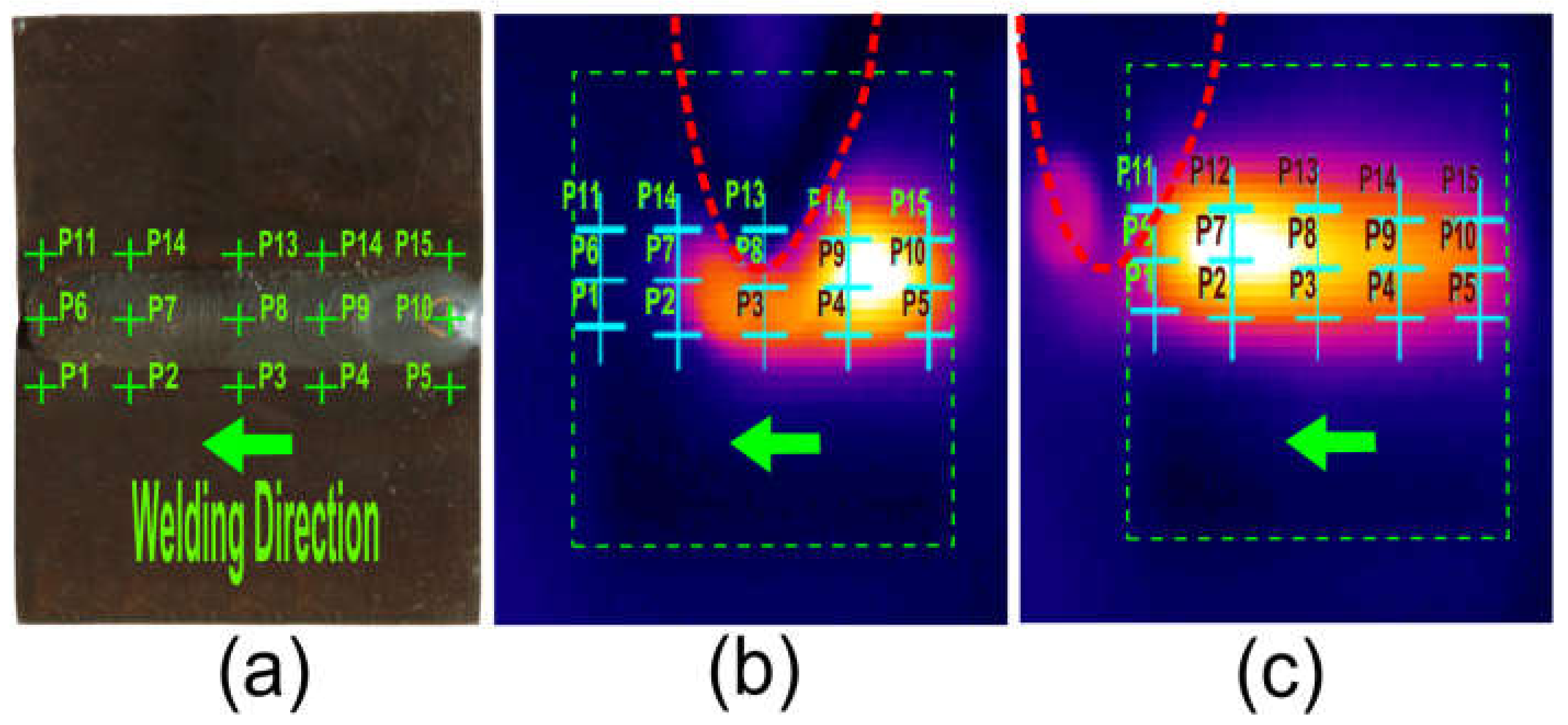
4.1. Measuring the Temperature Field

The angular distortion and the temperature field in the welding process can be used to validate the proposed FE models. These fields were used in the present paper to validate the three proposed FE models of a butt joint with a single V-groove. The temperature field during the welding process was determined for each of the key points of the welded joint as a function of time. This normally involves thermo-couples or Infrared Radiation (IR) technology, with a thermographic camera. The latter provides the temperature field automatically and accurately for all the points of the weld (plates and weld bead). IR technology has been used successfully by some investigators to determine the temperature field, and, then, to use the information to validate the welded joint FE models (Bzymek et al. [32]; Tonkovic’ et al. [33]; Perić et al. [34]). The temperature field for the present paper was recorded by IR technology, while the three single V-groove welded joints were manufactured. The field was recorded at two second intervals by a thermographic camera (Thermovision 570 AGEMA infrared system AB). The recording time of the temperature field was 100 s. This is sufficient time for the welded joints to cool considerably. Measurement of the temperature field was limited to the central points of the weld joint (i.e., P2, P3, P4, P7, P8, P9, P12, P13, and P14). Points P1, P5, P6, P10, P11, and P15, were not considered for validation of the FE models. This was due to a desire to avoid errors in the measurement of the temperature due to the transient starting and ending of the welding. Figure 2a shows the points for the measurement of the temperature field of the butt joint that has a single V-groove welded joint. Figure 2b illustrates the experimental temperature field of all the points in at second No. 6. There is in this figure a curve shaped preceding the weld point in the welding direction. It is the shadow of part of the torch of the welding machine (dashed red line). Figure 2c illustrates the same at second No. 20.

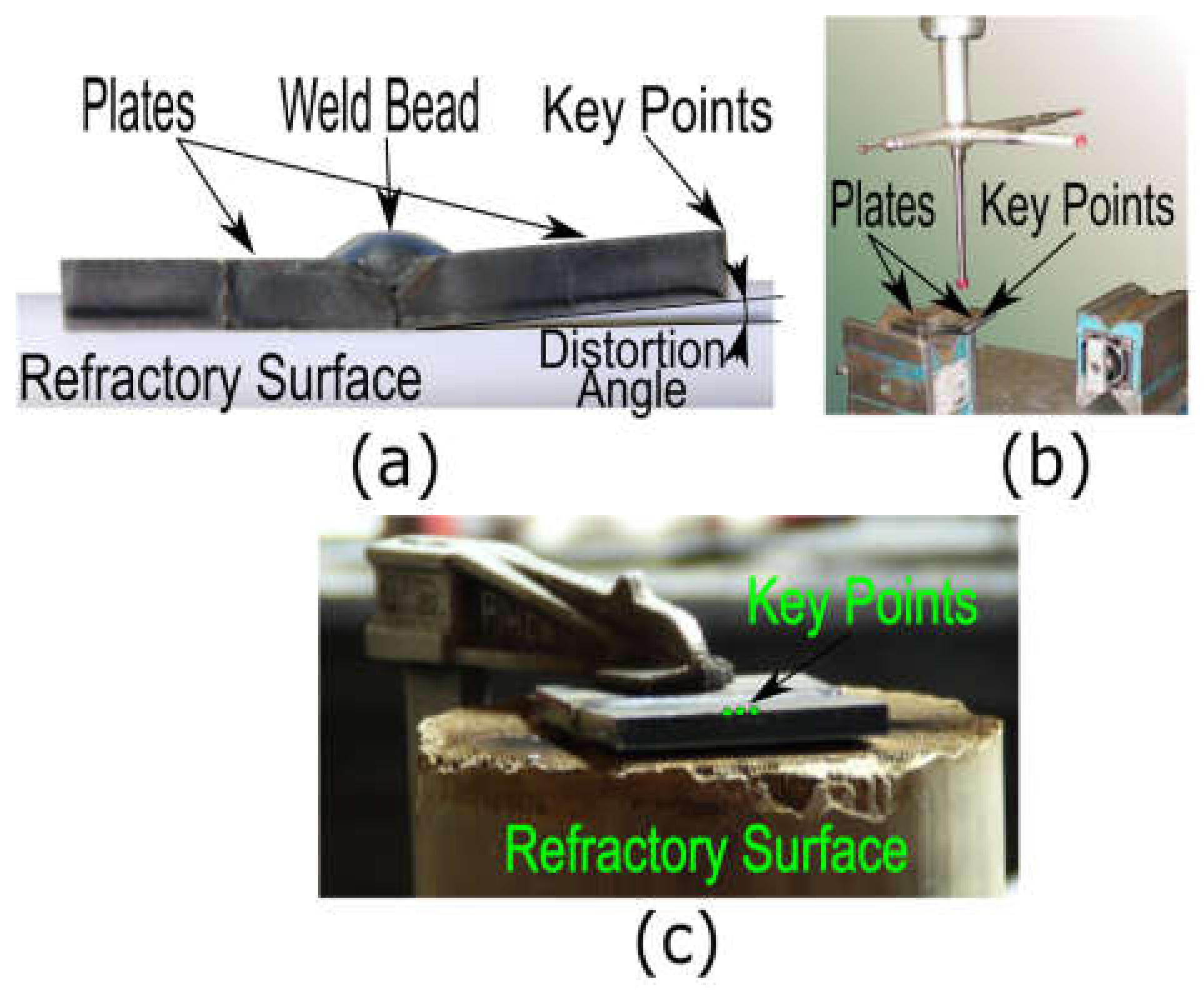
4.2. Measurement of Angular Distortion

Angular distortion is the result of non-uniform expansion and contraction of the weld cord and base metal during the heating and cooling cycle, which always appears in GMAW processes. Angular distortion is considered to be an indicator of residual stress to which the welded joint is subjected. The angular distortion should be avoided as much as possible, because if it is excessive, it can even affect the final dimensions of the mechanical component that is welded. In the current paper, the angular distortions of the three specimens that were studied were measured by use of a coordinate-measuring machine (model Zeiss PMC 850, Zeiss, Oberkochen, Germany) after the welded joints had cooled to room temperature. In this case, the angular distortions were measured by use of a selected group of key points on the edge of the plate that suffered most angular distortion in single V-groove welded joint (Figure 3a). These key points were located very close together in the central area of the welded joints, and served as a reference for measuring several times the angular distortion of each one of the studied specimens. This repeated measurement of the angular distortion was subsequently averaged to obtain a more realistic value. Figure 3b shows the coordinate-measuring machine that was used in the process of measuring the distortion angle. Figure 3c shows the key points that were used in each of the welded specimens to measure the angular distortion of the welded joint.

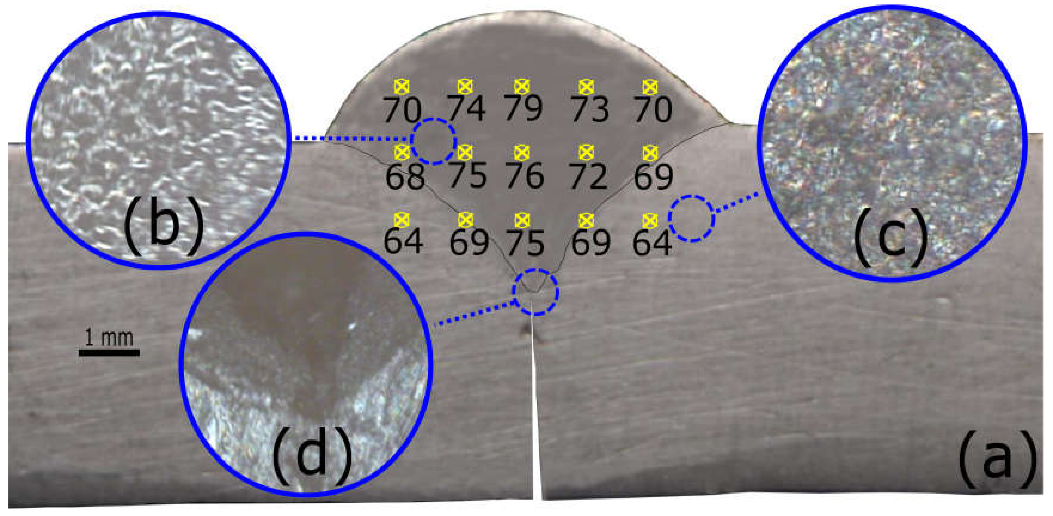
4.3. Characterization of the Welded Joint and Measurement of Weld Bead Geometry

Prior to conducting the characterization of the welded joint and the measurement of the weld bead geometry, X-ray radiographic analysis (ISO 17636 [35]) was undertaken with a Balteau X-ray radiographic machine. The analysis was undertaken as possible defects and imperfections were detected in the three specimens to be studied. In this case, if any of the specimens that were analyzed contained imperfections, it was rejected and was not used as a reference for the finite element model. Once the analyzed specimens showed no imperfection with the radiographic analysis, they were cut into pieces, and the faces of the cuts were polished and treated with picric acid in accordance with ASTM E407 [36]. This treatment ensured that the different areas of the welded joint (weld cord, base metal, and HAZ) were visible and could be identified. Then, the hardness was measured by a Hoyton Rockwell type 1003A durometer, according to ASTM E92 [37]. This enabled the detection of any phase transformation in the plates HAZ and weld bead. Using a diamond cone for the HRA scale in this case, a value of 60 kp was used for the three specimens. Figure 4a shows the hardness HV at various points of the base metal, weld cord, and HAZ for the first specimen. It shows a maximum hardness of 79 HRA, whereas the minimum hardness is 64 HRA. Also, Figure 4b–d shows the first sample’s transformation zones at a magnification of 40×. In Figure 4b, it can be seen that the bead is formed mainly by ferrite and perlite. Also, Figure 4c shows the composition of the base metal. It indicates that the base metal has a greater quantity of perlite than there is in the weld bead itself. Also, the HAZ (Figure 4d) shows a reduced area, which may be practically negligible. Similar phase changes and the affected areas were detected in the rest of the analyzed specimens. According to the results of the hardness measurement (Figure 4a) and of the metallographic analysis (Figure 4b–d), it can be deduced that no significant changes of phase were detected and that no important hard transformation zones for the three specimens studied were found (Barsoum [38]). This may be due to the low carbon content of both base material (EN 235JR) and weld bead (wire ER70S-6) that were used in this study, and also to the slow cooling of all the welded specimens (by air at room temperature and natural convection).

Then, the three welded joints were treated with picric acid, which caused the different areas to become visible; they were digitalized with a ZEISS microscope using a magnification of 40×. Then, the weld bead geometry that was essentially defined by the bead’s height, width, and shape was measured.

Table 2. Bead dimensions (height and width) and angular distortion of the welded specimens.

Inputs	Specimen 1	Specimen 2	Specimen 3
Height (mm)	1.3	1.5	2.5
Width (mm)	9.5	8.7	12.0
Angular Distortion (°)	4.64	4.723	4.934

shows the heights and widths of each of the three study specimens, as well as the angular distortion of each specimen. These data were then used to generate the FE models of each of the three welded joints that were studied.

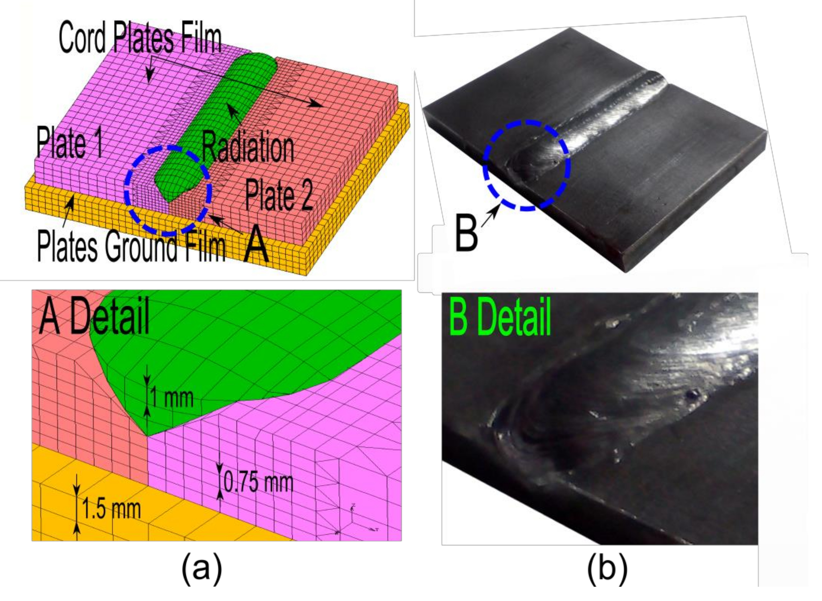
5. Finite Element Proposed for Modeling the Welded Joints

Over the years, most studies of welded joints that were based on FE models considered elastic-plastic material behavior, thermo-mechanical contacts, radiation, and convection in order to determine the distribution of displacements, distortions, and temperature. As the strains and stresses are determined as derivatives of displacement, the finite element shape functions for the displacements in thermo-mechanical problems generally should be greater by one order than for thermal analysis (Friedman et al. [39]; Friedman et al. [40]). Nevertheless, linear shape functions of elements are preferred. Low-order elements are more effective in solving nonlinear welded joint problems than larger high-order elements (Lindgren [41]). Also, fine mesh with linear elements is preferable for brick or hexahedral elements in three-dimensional models for plasticity problems (Benzley et al. [42]; Cifuentes et al. [43]). Hexahedral elements with functions of linear shape were used in the present paper. MSC Marc software [44] was used for simulation of the FE models of butt welded joints that have a single V-groove and to determine temperature fields and angular distortions. A total of 5200 elements were used to model the plates, 4536 elements to model the support plate, and 596, 546, and 642 elements to model the weld cords for the joints 1, 2, and 3, respectively. The input parameters and weld bead dimensions (height and width) in Table 1 and Table 2 were assumed in the development of the models. The proposed FE models did not consider the effects of phase transformation in the plastic strains, but a von Mises yield criterion with isotropic hardening rule was considered for base material and weld bead. The shape of the weld beads were experimentally obtained from the same cuts on the specimens studied in the characterization phase of the welded joint (See Section 4.3). Also, the FE models considered in their formulation to be linear shape functions with coupled thermal-mechanical fields and a temperature-dependent weld bead (wire ER70S-6) and base material (EN 235JR). According to Zhang et al. [14], the temperature-dependent material parameters were in this case the thermal expansion coefficient, thermal conductivity, elastic modulus, yield stress, and specific heat. These temperature-dependent materials were obtained from the MSC Marc software database [44]. Also, convection, conduction, and radiation were considered [21]. The addition of weld metal was modeled by the technique of birth and death of elements [12,45,46]. One plate was attached to a refractory surface (see Section 4 and Section 4.2). The other was supported on the refractory surface to deform freely from thermal shrinkage and stresses as the cord solidified and created angular distortion [11] (See Figure 5a). The three proposed FE models had the same height and width as the specimens that were welded and even modeled the web bead starting and ending zones (See Figure 5b). The minimum mesh size considered for the proposed models was 0.75 mm, 1.0 mm, and 1.5 mm for the plates, weld bead, and refractory surface, respectively.

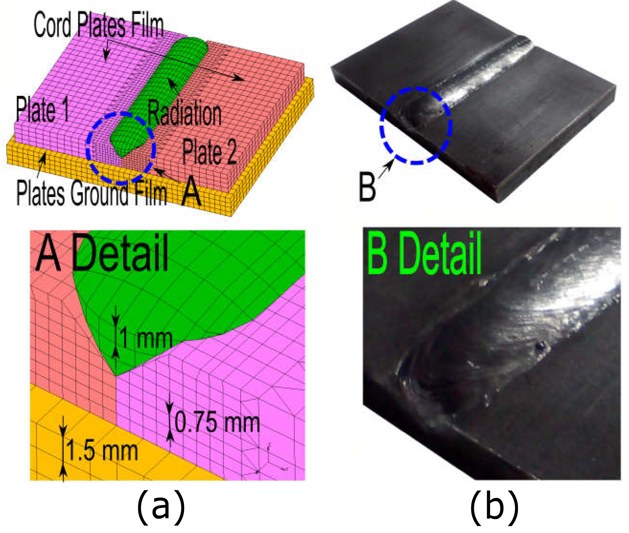
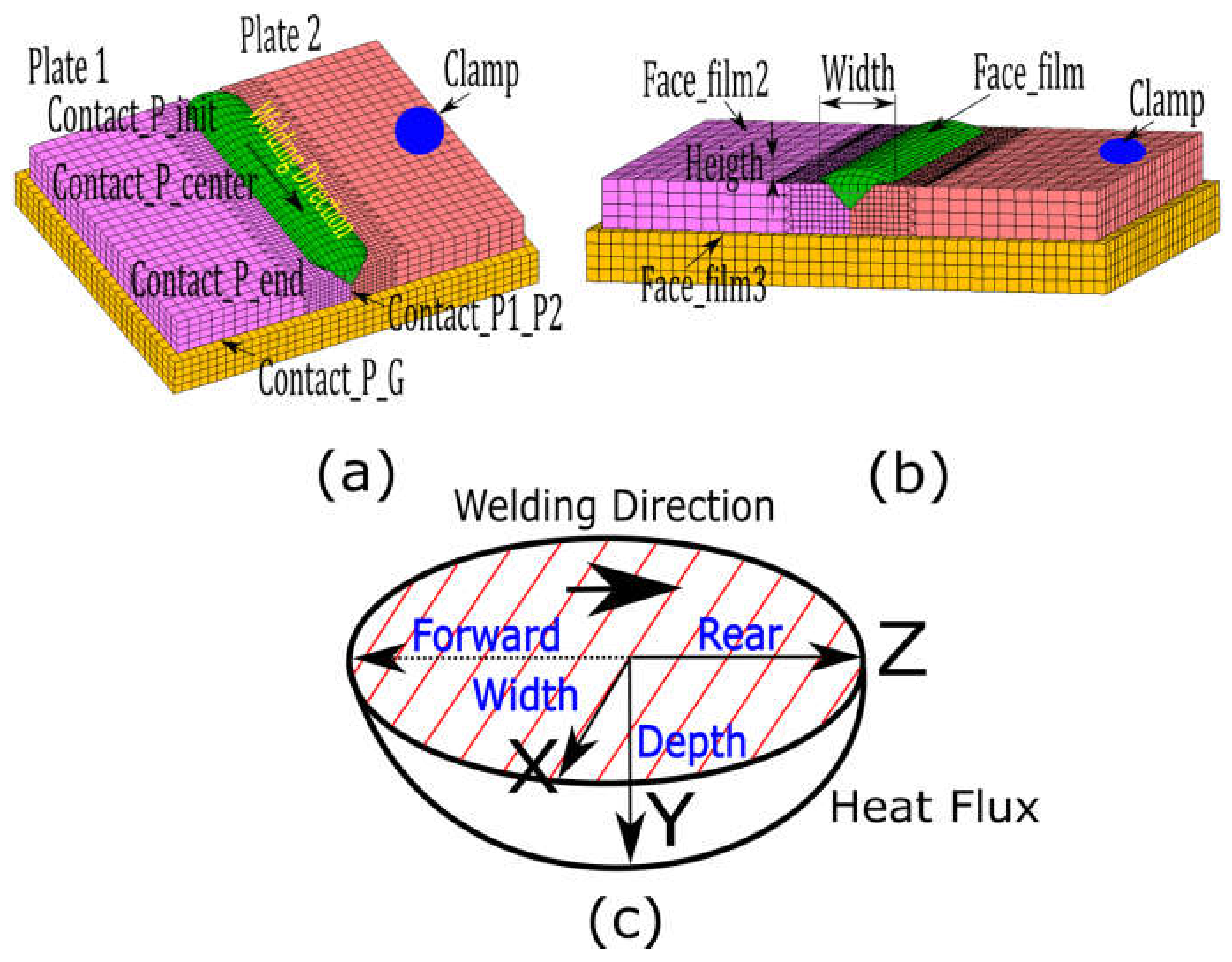
5.1. Parameterization of the Welded Joints FE Models

The three welded joint FE models were parameterized for the determination of the most appropriate parameters required to model the thermo-mechanical behavior. A total of thirteen parameters were considered to define the conduction and convection phenomena, as well as the weld flux. Firstly, the thermal conduction phenomena considered six parameters that were based on the different pairs of contacts that constituted the proposed welded joints. The introduction of thermal contact into the FE model provides the ability to take thermal conduction and small gaps into account. Bodies that are almost touching each other are considered to be in near contact. Different physical heat transfer processes, such as convection, natural convection, radiation, or distance dependent heat transfer can be simulated for this type of contact. A thermal contact analysis is undertaken when there is no structural pass. This results in a computationally more efficient analysis (MSC Marc software [44]). In this case, thermal contact Plate 1-Plate 2 (contact_P1_P2) and thermal contact plates-ground (contact_P_G) established the thermal contacts between the plates themselves, and, also, between the plates and the ground. Contact_P1_P2 has been included in this case, despite the existence at least at the beginning of the simulation, of a plane of geometric symmetry in the longitudinal direction of the weld bead. Plate 2 is fixed to the refractory surface by a clamp, whereas Plate 1 is free to rotate (See Figure 1b). In the beginning of the welding process, both plates are in contact with the refractory surface. In this situation, the heat transfer from Plate 1 and Plate 2 to its surroundings (air and a contact with the ground (convection and conduction)) is the same. With this condition, the Contact_P1_P2 could be not taken into consideration. As the welding process is being completed, the heat transfer from Plate 1 to its surroundings continues. However, the heat transfer from Plate 2 to its surroundings changes mainly to air (convection). In this new situation, the symmetry of the welding process would no longer be true and the elimination of Contact_P1_P2 would be a mistake. Also, three different thermal contacts were considered between the weld bead and the steel plates. This was raised to indicate that the dimensions of the weld bead are reduced, both at the beginning and the end of the welded joint in contrast to its central zone. For example, at the beginning of the weld cord was defined the weld cord-plates thermal contact (contac_P_init), whereas in the central zone, another weld cord-plates thermal contact (contac_P_center) was defined. Also, the weld cord-plate thermal contact was defined for the end zone of the cord (contac_P_end). Finally, the melting_point parameter corresponds to the melting temperature of the weld bead (melt_point). In the same way that the conduction coefficients were defined based on three different zones of the welded joint, three different convection coefficients were defined for modeling the phenomenon of thermal convection. The first region of the welded joint is the weld bead itself, the temperature of which is much higher than that of the rest of the joint. A first convection coefficient called face_film was defined as the thermal convection coefficient between the weld bead and the air. A second zone, in which the convection is produced in the welded joint, is that between the sides and the top of the two plates and air (face_film2). Finally, as the angular distortion causes the plate (Plate 1) that is not fixed to the refractory surface to begin to rotate, another convection zone appears in the welded joint. Another face_film3 is the coefficient of thermal convection between the air and the bottom of Plate 1. However, this plate was initially not in contact with air, but the refractory surface, instead. Also, it was assumed that the weld flux for all FE models had was a double ellipsoidal in shape according to Goldak [7], as it was necessary to adjust the parameters for: forward_length; rear_length; width and depth. These parameters are defined mainly to determine the weld flux rates per unit of volume in the weld pools, according to the double ellipsoidal. Forward_length and rear_length are the weld pool lengths in the welding direction, whereas the width and depth are the weld pool lengths in a direction that is perpendicular to the direction welding. Finally, the weld bead and surrounding areas were exposed to radiation by vision factors in the software (MSC Marc software [44]). Figure 6a shows the proposed thermal contacts to solve the conduction phenomenon in the FE model. Figure 6b provides the proposed thermal convection coefficients for solving the convection phenomena. Figure 6c shows the double ellipsoidal according to Goldak [7], in which the parameters of forward_length; rear_length; width and depth can be displayed.

As previously mentioned, the methodology proposed in this paper for adjust welded joints FE models could be used to adjust the thermo-mechanical behavior of any type of joint. In that case, the proposed FE models would have defined other parameters that are necessary to define the conduction and convection phenomena, as well as the weld flux.

5.2. Adjusting the Welded Joints FE Models

The proposed methodology for setting the best parameters for modeling Butt joint single V-groove weld FE models on the basis of angular distortion and temperature field with GA, as follows. First, the welded inputs of speed, current, and voltage (Table 1), the experimental temperature field and the angular distortion (Table 2) were selected for each of the three different welded joints that were studied. Subsequently, the ranges and step of the parameters to be adjusted and needed to model thermo-mechanical behavior in the welded joints FE models (in this case 13 parameters defined in Section 5.1) were established. Then, the GA process began to fix the objective functions of J_Temp and J_Dist based on Equations (2) and (3) for each of the individuals, generated as follows:

$$J_{Tempj}=\frac{{{\displaystyle \sum }}_{i=0}^n|T_{FEM}(i)-T_{EXP}(i)|}{{{\displaystyle \sum }}_{i=0}^n|T_{EXP}(i)-T_{Exp}(mean)|}$$

(2)

$$J_{Distj}=\frac{|{\alpha }_{FEM}-{\alpha }_{EXP}|}{{\alpha }_{EXP}}$$

(3)

In all the studies of Multi-objective Optimization, one of the main tasks is to define the objective functions in such a way that their maximum and minimum values that these functions can reach are of the same order of magnitude. These objective functions are often normalized with a common base. In this way, the process of maximizing or minimizing them is executed in a way that does not penalize or favor any of them excessively [47]. In this case, J_Temp and J_Dist were defined in a way that errors in the modeling of the temperature and in the modeling of angular distortion could were comparable and of a similar order of magnitude. The objective function J_Tempj (also known as Relative Absolute Error (RAE)) was defined as the average difference between the temperature obtained from each of the key nodes (n) that belong to the FE models (T_TFE(i)) and the temperature obtained from the thermographic camera (T_EXP(i)) at the homologous key points of the samples. In this case, the key nodes, P1, P5, P6, P10, P11, and P15, were not considered, as was mentioned in Section 4.1 due to a desire to avoid errors in measuring the temperature due to the transient starting and ending of the welding process. Instead, only the key nodes P2, P3, P4, P7, P8, P9, P12, P13, and P14 were considered for calculation of the temperature field. The J_Tempj functions that were obtained for the cited nine key points were examined at 2-s intervals from the beginning of the welding process at t = 0 s. to t = 100 s (See Figure 2). The subscript j represents the numbering of the welding cord that was studied. In this case, they range from 1 to 3. T_EXP(i) is the mean of experimental temperatures that were obtained at each of the nine key points that were studied. The objective function J_Distj was defined as the difference between the absolute value of the average angular distortion obtained from a selected group of key nodes del FE model (α_FEM) and the distortion angle that was obtained from the homologous key points of the tested samples (α_EXP). Weights w_Temp and w_Dist were applied to each of the objective functions J_Tempj and J_Distj, respectively, in order to consider the different adjustment requirements for the parameters of the proposed FE models. In this case, w_Temp was defined as being of a greater importance in the adjustment of the temperature field for the proposed FE model, whereas w_Dist was defined as being of greater importance in the adjustment of the angular distortion of that FE model. For example, if a minor error in the adjustment of the temperature field for the proposed FE model is permitted, but a greater error is permitted in the adjustment of the angular distortion of that model, the w_Temp and w_Dist may be assigned the following weight (major importance level assigned to the temperature field).

$$w_{Temp}=1.8\mathrm{and}{w}_{Dist}=0.2$$

Conversely, if a minor error in the adjustment of the angular distortion for the proposed FE models is permitted, but a greater error is permitted in the adjustment of the temperature field of that FE models, the w_Temp and w_Dist may be assigned the following weight (major importance level assigned to the angular distortion).

$$w_{Temp}=0.2\mathrm{and}{w}_{Dist}=1.8$$

In this way, the sum of both weights is equal to 2. In this paper, the fields of temperatures and the angular distortion have been considered to be equally important in adjusting the parameters of the proposed FE models. For this reason, w_Temp and w_Dist weights have each been assigned a value of 1.0.

Also, the sum of the two objective functions in relation to their respective weights is the overall objective function J_Total, which is the function to minimize. It is defined as follows:

$$J_{Totalj}=J_{Tempj}\times w_{Temp}+J_{Distj}\times w_{Dist}$$

(4)

Each of these objective functions was used to adjust each of the parameters of the welded joint FE models proposed (j = 3).

5.3. Crossovers and Mutations

After the objective functions were formulated and the welded inputs, experimental temperature field, and the angular distortion were established, the GA process began with the first generation (generation “0”) of individuals (i.e., FE models) that was randomly generated and simulated by the MSC Marc software [44]. Based on this process, the individuals of each generation were formed for the 13 features that were defined as input parameters. The data for each of these features were in decimal format. So, to obtain chromosomes with the right format, each digit of the input feature values (only decimal digits that can vary have space in the chromosomes) were transformed to binary code in order to use the GA method. During the transformation from the real values of the 13 features to binary code and during the transformation back from the binary code to real values, attention was given to removing possible values that were outside of the proposed range in the new offspring. The minimum and maximum values, the step and the format of each feature were considered. Because four binary digits formed a decimal code, the values that were obtained from new offspring in such cases were irrational, and, in other cases, outside of the ranges that were proposed in the study. Thus, such values were detected and removed from the process. Once the chromosome was in the correct format, the fitness function was calculated and the GA process continued as explained. In this case, the number of individuals that formed the first generation was 100 for each of the welded joints that were studied. After each individual from generation “0” was simulated, a correlation-based feature selection (CFS) [48,49] was made to determine which parameters most influenced the temperature field and the angular distortion. The objective of this analysis was to preset those parameters of least influence on the temperature field and angular distortion to the mean value of their range, and to adjust those more influential parameters by the crossing and mutation with GA. After each generation “0” individual was simulated, the objective function J_Totalj for each of the welded joints that were studied was evaluated by use of a script that was written in “R” language [50]. The best individuals of this generation “0” were those that had the lowest value of the objective function J_Totalj. The next generations (Generation 1 and subsequent generations) were created by crossing and mutation, as described below:

• 30% of the individuals with the lowest objective function J_Totalj values of the previous generation became parents of the new generation.
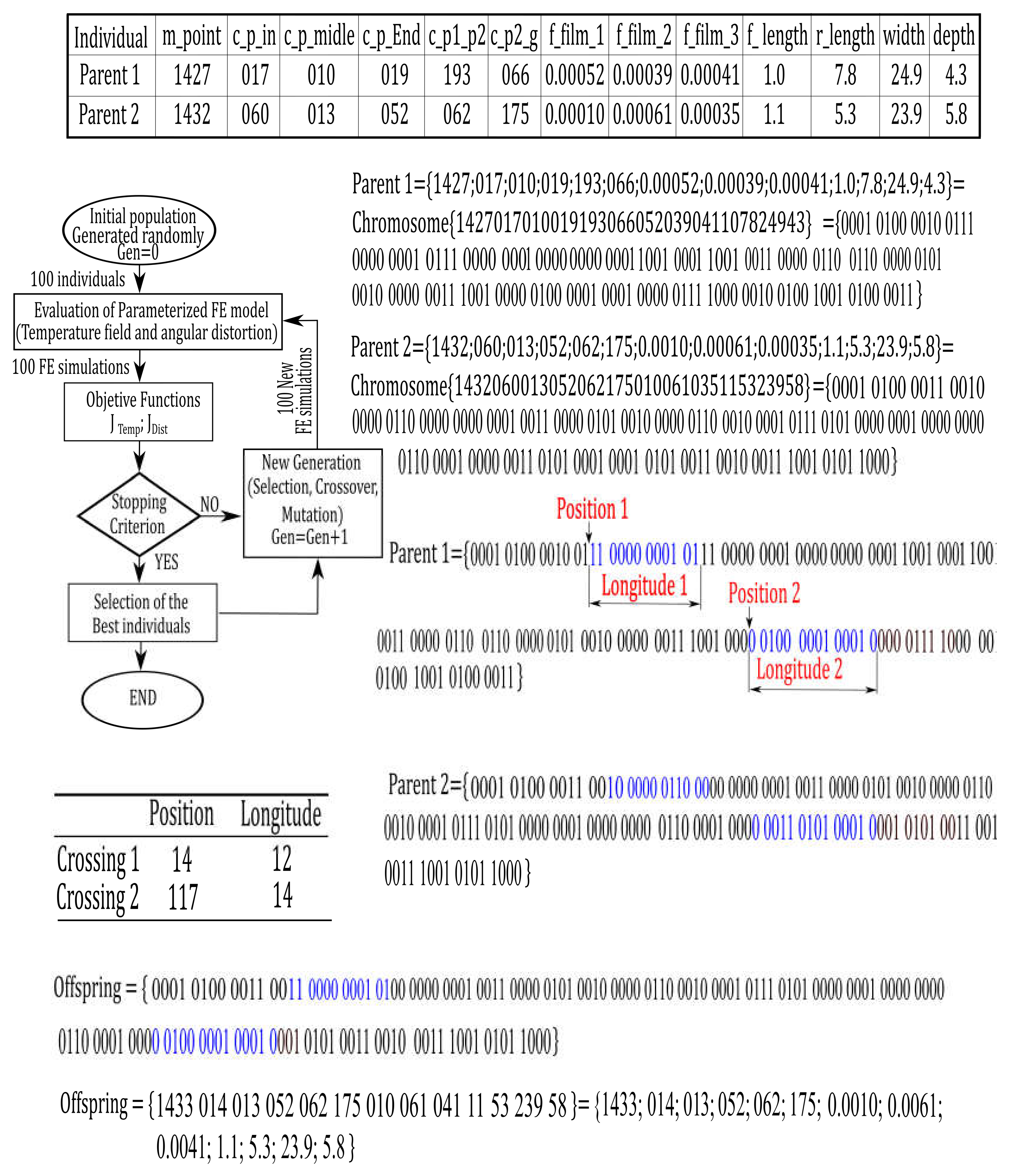
• 60% of individuals were created by crossing selected parents. The crossing was implemented by a script in “R” language [50]. It consists of a change in a random number of bits of chromosomes of two randomly selected best individuals. First, it was necessary to obtain two complete chromosomes from two selected parents. Then, each chromosome was coded to binary code to perform the process of crossing. Then, a random number of crossings (1, 2, 3, or 4) were selected. Also, for each crossing a position number that defined the position of the initial bit of each crossing was randomly selected too. In the same way, the longitude of the number of bits that form the crossing part of the chromosome was selected. With this information, some bits of the first parent were selected and the remaining bits were selected from the second parent to create a new chromosome for the next generation. Figure 7 shows the first and second positions 1 and 2, and the lengths (longitude 1) and (longitude 2) that were selected in this case for the crossing of two individuals from the generation “0”. In this case, position 1 was equal to “14” and position 2 was equal to “117”. Longitude 1 was equal to “12” and longitude was equal to “14” (all position and longitude values are in bits). Finally, the new chromosomes were decoded from their binary code to generate the new offspring that were formed by the parameters to be adjusted in order to model the thermo-mechanical behavior of the welded joints.
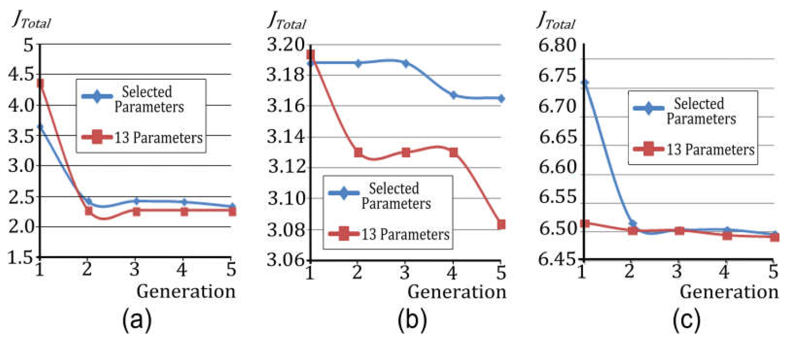
• The remaining 10% of individuals were obtained by mutation. A random number of bits (between one and the number that defines the longitude of the chromosome) are defined and random positions of the chromosome are selected and are commuted until reaching the number of the initial number of bits selected. Meanwhile, it was important to always check that the new randomly generated values were within the established ranges. The aim of generating individuals by mutation was to find new solutions in areas that had not been explored previously. This procedure was repeated separately for each of the welded joints that were studied for several generations until the objective function J_Totalj no longer increased significantly.

5.4. Correlation-Based Feature Selection

Correlation−based feature selection (CFS) is a simple rank filter algorithm that select features according to a heuristic evaluation based on a correlation function [48,49]. The feature subset evaluation function is shown in Equation (5).

$$Meri{t}_s=\frac{k·\overline{r_{cf}}}{\sqrt{k+k·(k-1)·\overline{r_{ff}}}}$$

(5)

where Merit_s is the heuristic merit of a feature subset S containing k features, $\overline{r_{cf}}$ is the mean feature-class correlation, and $\overline{r_{ff}}$ is the mean feature-feature intercorrelation. The numerator indicates how a group of features predicts a numeric class and the denominator of the redundancy among the features. This technique was applied as a feature selector because of its low computational cost and simplicity of use.

6. Case Study

This section presents a case study of the determination of the best parameters for modeling a Butt joint single V-groove weld manufactured by the one-pass Gas Metal Arc Welding (GMAW) process with different welded inputs of voltage and current (See Table 1), and weld bead dimensions of height and width (See Table 2).

6.1. Results That are Based on CFS

CFS was used to assess the uncertainty of the input parameters respect to the J_Total objective function that was obtained from the three welded FE simulations. The CFS filter algorithm was used on a sample of 100 individuals or 100 FE simulations when considering the aforementioned 13 input parameters, which were randomly generated.

Table 3. Range considered for each of the input parameters of the FE models studied.

Range of	Melt Point	Contact P_init	Contact P_center	Contact P_end	Contact P1_P2	Contact P_G	Face_Film
Parameters	(°C)	(N/s·°K)	(N/s·°K)	(N/s·°K)	(N/s·°K)	(N/s·°K)	(N/s·°K·mm)
Min.	1420	1	1	1	1	1	0.00001
Max.	1440	300	700	300	200	200	0.00100
Step	1	1	1	1	1	1	0.00001
Range of	Face_film2	Face_film3	Forward Length	Rear Length	Width	Depth	-
Parameters	(N/s·°K·mm)	(N/s·°K·mm)	(mm)	(mm)	(mm)	(mm)	-
Min.	0.00001	0.00001	1.0	5.0	23.0	4.0	-
Max.	0.00100	0.00100	2.0	10.0	26.0	6.0	-
Step	0.00001	0.00001	0.1	0.1	0.1	0.1	-

shows the range of values that were considered for each of the input parameters of the FE models studied to generate the 100 individuals. The range was the same for each of the three welded joints FE models studied and was based on experience that was gained in previous research work [11,19,20].

Table 4. Results of using the correlation based feature selection (CFS) technique to analyze the relationship between the output feature or objective function J_Totalj and the input parameters.

Inputs	First FE Model	Second FE Model	Third FE Model
melt_point	-	-	-
contac_p_in.	-	-	-
contac_p_midle	X	-	-
contac_p_End	-	-	X
contact_p1_p2	-	-	-
contact_p2_Ground	-	-	-
face_film	-	-	-
face_film2	-	-	-
face_film3	-	-	-
forward_lenght	-	-	X
rear_lenght	X	X	X
width	-	-	-
depth	-	-	-

shows the results of using the CFS technique to analyze the relationship between the output feature and “objective function J_Totalj” for each of the three FE models of welded joints proposed, and the 13 inputs parameters. The results show the most significant parameters of the FE models that were selected in each case.

The first column of Table 4 shows the most significant input parameters that were selected for the first proposed FE model (current = 140 amps and voltage = 26.0 volts). In this case, it can be seen that the “contac_p_midle” and the “rear_lenght” parameters are the most influential inputs for the objective function J_Total1. The second column of this table shows the most significant features that were selected for the second proposed FE model (current = 210 amps and voltage = 28.0 volts). It can be seen that it is the “rear_lenght” parameter in the input that most influences the objective function J_Total2. Finally, the third column of this table shows the most significant features that were selected for the third proposed FE model (current = 260 amps and voltage = 35.0 volts). In this case, “rear_lenght”, “contac_p_End”, and “forward_lenght” are the parameters that most influence the objective function J_Total3.

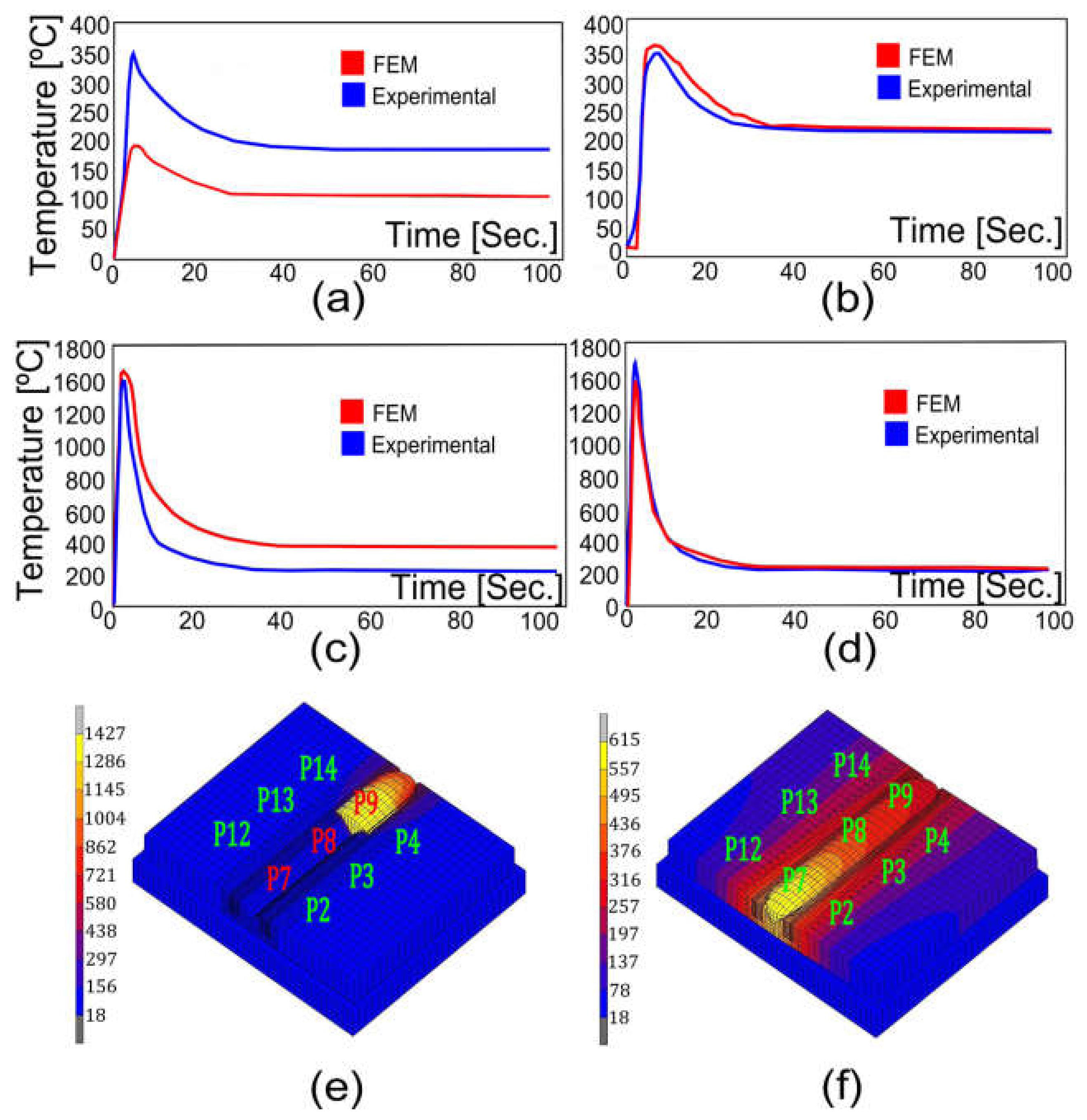
6.2. Results of FE Model Adjustment

The adjustment process that uses GA to set the parameters of Butt joint single V-groove welded FE models that were manufactured with different welded input of speed, voltage, and current were developed in two different ways. The first way with GA only considered the most influential parameters that were selected from the CFS filter algorithm (See Table 4). That is, for the first proposed welded joint, the parameters that were adjusted by GA were two parameters (“contac_p_midle” and the “rear_length”). For the second proposed welded joint, there was only one parameter (“rear_length”). However, for the third weld, there were three parameters (“rear_length”, “contac_p_End”, and “forward_length”). The remaining least influential parameters for the objective function J_Total were initially set at the mean value of the range studied and were not adjusted by GA. The second way of adjusting the parameters of the three welded joints that were studied considered the totality of the 13 parameters that were proposed. Figure 8 shows the development of the J_Totalj of the best individual in each generation. As was mentioned in Section 5.2, the development assumes the same level of importance for the thermal field as for the angular distortion (w_Temp = 1 and w_Dist = 1). Figure 8a–c shows the development of the J_Total for the best individual when considering the 13 parameters that define the thermo-mechanical behavior of the welded proposed joints FE models. Also, these figures show the development of the J_Totalj for the best individual when only those parameters of most influence are considered when they are analyzed and selected by the CFS filter algorithm. An examination of all the figures revealed that the first welded joint FE model that was studied provided lower values of J_Total (See Figure 8a) than the remaining welded joint FE models that were proposed. In addition, it is seen in these figures that the minimum values reached for J_Totalj always correspond in cases when the 13 parameters that define the thermo-mechanical behavior of the proposed welded joints FE models are considered. Also, Figure 8a provided lower values of J_Total than the remaining FE models that were proposed for the various requirements that were studied. This means that the first FE model’s settings of the 13 parameters are higher than those of the parameters in the other FE models. It was also noted that the stabilization of J_Total was achieved within a few generations (five generations) in all of the cases studied, although the number of parameters of the FE model is very high.

Also,

Table 5. Results of the adjustment process for the three welded joints FE models: considering the 13 input parameters and considering the selected parameters by the CFS filter algorithm.

Ways to Adjust	FE	Gen.	Melt	Contact	Contact	Contact	Contact	Contact	Face	Face	Face	Forward	Rear	Width	Depth	JTotal
	Weld	-	Point	P_init	P_center	P_end	P1_P2	P_G	Film	Film_2	Film_3	Length	Length	-	-	-
	-	-	(°C)	(N/(s·K))	(N/(s·K))	(N/(s·K))	(N/(s·K))	(N/(s·K))	(N/(s·°K·mm))	(N/(s·°K·mm))	(N/(s·°K·mm))	(mm)	(mm)	(mm)	(mm)	-
CFS algorithm	1	01	1430	150.5	2	150.5	100.5	100.5	0.000505	0.000505	0.000505	1.5	9.7	24.5	5.0	3.6652
		05	1430	150.5	13	150.5	100.5	100.5	0.000505	0.000505	0.000505	1.5	5.3	24.5	5.0	2.3416
	2	01	1430	150.5	350.5	150.5	100.5	100.5	0.000505	0.000505	0.000505	1.5	6.7	24.5	5.0	3.1879
		05	1430	150.5	350.5	150.5	100.5	100.5	0.000505	0.000505	0.000505	1.5	6.5	24.5	5.0	3.1654
	3	01	1430	150.5	350.5	163	100.5	100.5	0.000505	0.000505	0.000505	1.3	6	24.5	5.0	6.7602
		05	1430	150.5	350.5	174	100.5	100.5	0.000505	0.000505	0.000505	1.7	5.2	24.5	5.0	6.4968
13 parameters	1	01	1431	102	2	219	193.0	62.0	0.00051	0.00047	0.00051	1.4	7.8	24.8	4.3	4.3917
		03	1427	17	10	19	193.0	66.0	0.00052	0.00039	0.00041	1.0	7.8	24.9	4.3	2.2680
	2	01	1423	164	107	130	115.0	118.0	0.00055	0.00004	0.00011	1.4	7.5	26	5.1	3.1938
		03	1425	257	65	189	195.0	176.0	0.00071	0.00039	0.00033	1.8	7.4	23.8	4.3	3.0838
	3	01	1429	162	582	198	127.0	83.0	0.00095	0.0008	0.0007	1.6	5.4	25.3	4.6	6.5161
		03	1429	203	662	247	159.0	182.0	0.00093	0.0008	0.00068	1.6	5.2	23.1	5.4	6.4918

shows the thirteen input parameters that were obtained for each of the three FE models to define the thermal conduction and thermal convection phenomenon when the values of J_Total no longer increased significantly for each of the generations and for the two different ways that were proposed. For the 5th generation of the first specimen studied, it can be seen that the value of J_Total with the 13 parameters reaches a value of 2.268, but reaches a value of 2.3416 with a selection of parameters by the CFS filter algorithm. This difference between J_Total increases as the power supplied to the welded joint increases (See Table 1). So, for example, J_Total reaches a value of 3.0838 for the second specimen studied with the 13 parameters, but reaches a value of 3.1654 with the parameters that were selected with CFS filter algorithm. For the third specimen, J_Total reached values of 6.4968 and 6.4918 with the 13 parameters and the selection of parameters by the CFS filter algorithm, respectively. This difference in the values reached by J_Total suggests that the parameters of the proposed welded joints FE models provide a better fit when the power supplied to the welded joint is lower. Analyzing the values that were achieved for the 13 parameters in their adjustment process (with the CFS filter algorithm), the unique parameter that is common to the three welded joints studied (rear_length) decreases as the power supplied to the welded joint increases (7.8, 7.4, and 5.2). However, analyzing the values achieved for the 13 parameters in their adjustment process (with the 13 parameters), it is seen that: higher melting point values (melting_point), thermal contacts between the weld bead and both plates for the central zone, and the end zone of the bead (contac_P_center and contac_P_end) and thermal contact between plates 1 and 2 with the ground (contact_P_G) generally increased as the power that was supplied to the welded increased. For example, the melting_point varied from 1427 to 1429, whereas the values for contact_P_end, contact_P_center, and contact_P_G varied from 19 to 247, from 10 to 662, and from 66 to 182, respectively. Furthermore, the values that achieve the objective function increased as the power supplied increased. This means that the models provide a better fit when the power that is supplied to the welded joint is lower. Also, analyzing the results of the adjustment of the two procedures proposed, rear_length is the unique parameter that is common to all of them, and, therefore, is one of the most influential parameters in the adjustment of the proposed welded joint FE models. As previously mentioned, rear_length is defined mainly to determine the weld flux rates per unit of volume in the weld pools, according to the double ellipsoidal theory, and is the weld pool length in the welding direction (back of the melting point). In this case, according to Figure 6c and Table 5, the rear_length is always much greater than the forward_length. This suggests a greater area of weld flux rates per unit of volume contributed in the weld pools behind the melting point. In turn, this suggests that the adjustment of the models of FE of the welded joints proposed could be mainly focused on the adjustment of the contribution of the weld flux rates behind in the back of the melting point.

Figure 9 illustrates the process of adjustment for the first FE model of a butt joint with single V-groove that was used for study of the temperature of key nodes 14 and 9 (at the weld bead base and on the weld bead, respectively). Figure 9a,b compares the temperatures of key nodes P14 and P9, which were obtained experimentally by thermographic camera, and that of the FE model in 100 s without adjusting the FE model’s parameters. Similarly, Figure 9c,d provides the corresponding temperatures for key nodes P14 and P9 and the FE model’s parameters optimized for this same first welded joint studied. Also, Figure 9e,f shows the temperature field after 3 s and 100 s of simulation, respectively, for the first welded joint FE model that was studied. Similarly, Figure 9f shows the maximum angular distortion of the welded joint model after 100 s of simulation.

Table 6. Values of the angular distortion obtained with the proposed FE models and experimentally by use of a coordinate-measuring machine.

Specimen	FEM (°)	Experimental (°)	Error (%)
1	4.73	4.64	4.11
2	4.92	4.723	4.17
3	5.21	4.934	5.59

shows the angular distortions of each of these FE models studied, the angular distortion obtained experimentally using a coordinate-measuring machine and the error, as well as the error by each of the FE models. The table indicates that specimen 3 produced the greatest error (5.59%) and specimen 1 gave the smallest error (5.11%).

7. Conclusions

To ensure realistic results in modeling the welded joints using the FEM, it is essential to appropriately characterize the thermo-mechanical behavior of the elastic-plastic Finite Element (FE) models. This paper sets out a methodology to determine the most appropriate parameters for modeling the thermo-mechanical behavior of Butt joint single V-groove FE models that were manufactured by the one-pass Gas Metal Arc Welding (GMAW). As a practical example, the proposed methodology is validated on three different welded joints specimens that were manufactured with different voltages and currents (26 volts and 140 amps; 28 volts and 210 amps; and, 35 volts and 260 amps). The base material was, for all of the specimens manufactured, was EN 235JR low carbon steel, whereas the weld bead was ER70S-6 steel. The electrode orientation, shielding gas flow rate, distance between nozzle and plate, and welding speed were, for all of the fabricated specimens, from 80°, 20.0 L/min, 4.0 mm, and 6 mm/s, respectively. An objective function J_Totalj was defined for each of the proposed welded joints as the combination of an objective function based on the temperature field J_Tempj and an objective function based on the angular distortion J_Distj. Weights w_Temp and w_Dist were applied to each of the objective functions J_Tempj and J_Distj, respectively, in order to consider different adjustment requirements for the parameters of the proposed FE models. w_Temp was defined as having greater importance in the adjustment of the temperature field, whereas w_Dist was defined as having greater importance in the adjustment of the angular distortion. In this case, both the field of temperatures and the angular distortion were considered to be equally important in adjusting the parameters of the proposed FE models. Value of 1.0 was assigned to w_Temp and w_Dist respectively. Two different ways to adjust the parameters were proposed. They were (1) using a feature selection of the parameters that most influence the objective function J_Total after applying to (CFS) filter algorithm; and, (2) using all of the 13 parameters for the three welded joint FE models. In analyzing the results of the adjustment of the two proposed procedures, it was seen that: (1) The rear_length is the parameter that is common to all, and, therefore, is one of the most influential parameters; (2) The differences in the values reached by J_Total suggest that the parameters of the welded joints FE models provide a better fit when the power supplied to the welded joint is lower. In this case, the rear_length is always much greater than the forward_length. This suggests a greater area of weld flux rates per unit of volume contributed in the weld pools of the back of the melting point. In turn, this suggests that the adjustment of the models of FE of welded joints proposed could be focused mainly on the adjustment of the weld flux rates that contributed in the back of the melting point. Finally, we can say that the methodology that is proposed in this paper could be valid for adjusting the parameters that define the thermo-mechanical behavior of any type of welded joint FE models. In that case, the parameters that are needed to define the conduction and convection phenomena, as well as the weld flux of that welded joints FE models, would be defined differently than what this work proposes, and would depend on the type of welded joint that is studied.

References

1. Macherauch, E.; Kloos, K.H. Origin, measurements and evaluation of residual stresses. In Residual Stress in Science and Technology, 1st ed.; DGM Verlag: Oberursel, Germany, 1987. [Google Scholar]
2. Ozcelik, S.; Moore, K. Modeling, Sensing and Control of Gas Metal Arc Welding, 1st ed.; Elsevier Science Ltd.: Kidlington, Oxford, UK, 2003. [Google Scholar]
3. Citarella, R.; Carlone, P.; Lepore, M.; Sepe, R. Hybrid technique to assess the fatigue performance of multiple cracked FSW joints. Eng. Fract. Mech. 2016, 132, 38–50. [Google Scholar] [CrossRef]
4. Citarella, R.; Carlone, P.; Sepe, R.; Lepore, M. DBEM crack propagation in friction stir welded aluminum joints. Adv. Eng. Softw. 2016, 101, 50–59. [Google Scholar] [CrossRef]
5. Lostado, R.; Martínez-de-Pisón, F.J.; Fernández, R.; Fernández, J. Using genetic algorithms to optimize the material behaviour model in finite element models of processes with cyclic loads. J. Strain Anal. Eng. 2011, 46, 143–159. [Google Scholar] [CrossRef]
6. Deng, D.; Murakawa, H. Numerical simulation of temperature field and residual stress in multi-pass welds in stainless steel pipe and comparison with experimental measurements. Comput. Mater. Sci. 2006, 37, 269–277. [Google Scholar] [CrossRef]
7. Goldak, J.A.; Akhlaghi, M. Computational Welding Mechanics, 1st ed.; Springer Science & Business Media, Inc.: New York, NY, USA, 2006. [Google Scholar]
8. Brickstad, B.; Josefson, B.L. A parametric study of residual stresses in multi-pass butt-welded stainless steel pipes. Int. J. Press. Vessels Pip. 1998, 75, 11–25. [Google Scholar] [CrossRef]
9. Ericsson, M.; Nylén, P. A look at the optimization of robot welding speed based on process modeling. Weld. J.-N. Y. 2007, 86, 238. [Google Scholar]
10. Attarha, M.J.; Sattari-Far, I. Study on welding temperature distribution in thin welded plates through experimental measurements and finite element simulation. J. Mater. Process. Technol. 2011, 211, 688–694. [Google Scholar] [CrossRef]
11. Lostado, R.; Corral, M.; Martínez, M.Á.; Villanueva Roldán, P.M. Residual Stresses with Time-Independent Cyclic Plasticity in Finite Element Analysis of Welded Joints. Metals 2017, 7, 136. [Google Scholar] [CrossRef]
12. Bachorski, A.; Painter, M.J.; Smailes, A.J.; Wahab, M.A. Finite-element prediction of distortion during gas metal arc welding using the shrinkage volume approach. J. Mater. Process. Technol. 1999, 92, 405–409. [Google Scholar] [CrossRef]
13. Pilipenko, A. Computer Simulation of Residual Stress and Distortion of Thick Plates in Multielectrode Submerged Arc Welding: Their Mitigation Techniques. Ph.D. Thesis, Department of Machine Design and Materials Technology, Norwegian University of Science and Technology, Trondheim, Norway, 2001. [Google Scholar]
14. Zhang, H.; Zhang, G.; Cai, C.; Gao, H.; Wu, L. Fundamental studies on in process controlling angular distortion in asymmetrical double-sided double arc welding. J. Mater. Process. Technol. 2008, 205, 214–223. [Google Scholar] [CrossRef]
15. Aarbogh, H.M.; Hamide, M.; Fjaer, H.G.; Mo, A.; Bellet, M. Experimental validation of finite element codes for welding deformations. J. Mater. Process. Technol. 2010, 210, 1681–1689. [Google Scholar] [CrossRef] [Green Version]
16. Chao, Y.J.; Zhu, X.; Qi, X. WELDSIM-A Welding simulation Code for the Determination of Transient and Residual Temperature, Stress, and Distortion. Adv. Comput. Eng. Sci. 2000, 2, 1207–1211. [Google Scholar]
17. Tian, L.; Luo, Y.; Yang, W.; Wu, X. Prediction of transverse and angular distortions of gas tungsten arc bead-on plate welding using artificial neural network. Mater. Des. 2013, 54, 458–472. [Google Scholar] [CrossRef]
18. Perić, M.; Tonković, Z.; Garašić, I.; Vuherer, T. An engineering approach for a T-joint fillet welding simulation using simplified material properties. Ocean Eng. 2016, 128, 13–21. [Google Scholar] [CrossRef]
19. Lostado, R.; Escribano, R.; Martínez, M.Á.; Múgica, R. Improvement in the Design of Welded Joints of EN 235JR Low Carbon Steel by Multiple Response Surface Methodology. Metals 2016, 6, 205. [Google Scholar] [CrossRef]
20. Lostado, R.; Fernandez, R.; Mac Donald, B.J.; Villanueva, P.M. Combining soft computing techniques and the finite element method to design and optimize complex welded products. Integr. Comput.-Aid. Eng. 2015, 22, 153–170. [Google Scholar]
21. Lostado, R.; Roldán, P.V.; Fernandez, R.; Mac Donald, B.J. Design and optimization of an electromagnetic servo braking system combining finite element analysis and weight-based multi-objective genetic algorithms. J. Mech. Sci. Technol. 2016, 30, 3591–3605. [Google Scholar] [CrossRef]
22. Gentils, T.; Wang, L.; Kolios, A. Integrated structural optimisation of offshore wind turbine support structures based on finite element analysis and genetic algorithm. Appl. Energy 2017, 199, 187–204. [Google Scholar] [CrossRef]
23. Duan, L.; Xiao, N.C.; Li, G.; Cheng, A.; Chen, T. Design optimization of tailor-rolled blank thin-walled structures based on-support vector regression technique and genetic algorithm. Eng. Optim. 2017, 49, 1148–1165. [Google Scholar] [CrossRef]
24. Bag, S.; De, A. Development of a three-dimensional heat transfer model for the gas tungsten arc welding process using the finite element method coupled with a genetic algorithm based identification of uncertain input parameters. Metall. Mater. Trans. A 2008, 39, 2698–2710. [Google Scholar] [CrossRef]
25. Voutchkov, I.; Keane, A.J.; Bhaskar, A.; Olsen, T.M. Weld sequence optimization: The use of surrogate models for solving sequential combinatorial problems. Comput. Method. Appl. Mech. Eng. 2005, 194, 3535–3551. [Google Scholar] [CrossRef]
26. Xie, L.S.; Hsieh, C. Clamping and welding sequence optimisation for minimising cycle time and assembly deformation. Int. J. Mater. Prod. Technol. 2002, 17, 389–399. [Google Scholar] [CrossRef]
27. Michalewicz, Z. GAs: What Are They? In Genetic Algorithms + Data Structures = Evolution Programs; Springer: Berlin, Heidelberg, Germany, 1994. [Google Scholar]
28. Fonseca, C.M.; Fleming, P.J. Genetic algorithms for multiobjective optimization: Formulation discussion and generalization. In Proceedings of the 5th International Conference on Genetic Algorithms (ICGA’ 93), Urbana-Champaign, IL, USA, 17–21 July 1993; pp. 416–423. [Google Scholar]
29. Minnick, H.M. Gas Metal Arc Welding Handbook Textbook, 1st ed.; Goodheart–Willcox: Tinley Park, IL, USA, 2007. [Google Scholar]
30. Murray, P.E. Selecting parameters for GMAW using dimensional analysis. Weld. J. 2002, 81, 125–131. [Google Scholar]
31. Grong, O. Metallurgical Modelling of Welding. Institute of Materials, 1st ed.; Carlton House Terrace: London, UK, 1997. [Google Scholar]
32. Bzymek, A.; Czuprýnski, A.; Fidali, M.; Jamrozik, W.; Timofiejczuk, A. Analysis of images recorded during welding processes. In Proceedings of the 9th International Conference on Quantitative InfraRed Thermography, Krakow, Poland, 2–5 July 2018. [Google Scholar]
33. Tonkovic´, Z.; Peric´, M.; Surjak, M.; Garašic´, I.; Boras, I.; Rodic´, A.; Švaic´, S. Numerical and experimental modeling of a T-joint fillet welding process. In Proceedings of the 11th International Conference on Quantitative InfraRed Thermography, Naples, Italy, 11–14 June 2012. [Google Scholar]
34. Perić, M.; Tonković, Z.; Rodić, A.; Surjak, M.; Garašić, I.; Boras, I.; Švaić, S. Numerical analysis and experimental investigation of welding residual stresses and distortions in a T-joint fillet weld. Mater. Des. 2014, 53, 1052–1063. [Google Scholar] [CrossRef]
35. ISO 17636-1:2013 Non-Destructive Testing of Welds–Radiographic Testing—Part 1: X- and Gamma-Ray Techniques with Film. Available online: https://www.iso.org/standard/52981.html (accessed on 9 January 2018).
36. ASTM E407-07. Standard Practice for Microetching Metals and Alloys. Available online: https://zh.scribd.com/document/259609551/ASTM-E407-07-StandardPractice-for-Microetching-Metals-and-Alloys (accessed on 9 January 2018).
37. ASTM E92-16. Standard Test Methods for Vickers Hardness and Knoop Hardness of Metallic Materials. Available online: http://www.astm.org/Standards/E92 (accessed on 9 January 2018).
38. Barsoum, Z. Residual stress prediction and relaxation in welded tubular joint. Weld. World 2007, 51, 23–30. [Google Scholar] [CrossRef]
39. Friedman, E. Thermomechanical analysis of the welding process using the finite element method. J. Press. Vessel Technol. 1975, 97, 206–213. [Google Scholar] [CrossRef]
40. Friedman, E. Numerical simulation of the gas tungsten-arc welding process. In Proceedings of the Numerical Modeling of Manufacturing Processes, ASME Winter Annual Meeting, Atlanta, GA, USA, 27 November–2 December 1977. [Google Scholar]
41. Lindgren, L.E. Computational Welding Mechanics: Thermomechanical and Microstructural Simulations, 1st ed.; Woodhead Publishing: Cambridge, UK, 2007. [Google Scholar]
42. Benzley, S.E.; Perry, E.; Merkley, K.; Clark, B.; Sjaardama, G. A comparison of all hexagonal and all tetrahedral finite element meshes for elastic and elasto-plastic analysis. In Proceedings of the 4th International Meshing Roundtable, Sandia National Laboratories, Albuquerque, NM, USA, 16–17 October 1995. [Google Scholar]
43. Cifuentes, A.O.; Kalbag, A. A performance study of tetrahedral and hexahedral elements in 3-D finite element structural analysis. Finite Elem. Anal. Des. 1992, 12, 313–318. [Google Scholar] [CrossRef]
44. MSC Mentat Marc. MSC. MARC User Guide; Version 2010; MSC. Software Corporation: Santa Ana, CA, USA, 2010. [Google Scholar]
45. Armentani, E.; Esposito, R.; Sepe, R. Finite element analysis of residual stresses on butt welded joints. In Proceedings of the 8th Biennial ASME Conference on Engineering Systems Design and Analysis, ESDA2006, Torino, Italy, 4–7 July 2006. [Google Scholar]
46. Armentani, E.; Esposito, R.; Sepe, R. The influence of thermal properties and preheating on residual stresses in welding. Int. J. Comput. Mater. Sci. Surf. Eng. 2007, 1, 146–162. [Google Scholar] [CrossRef]
47. Lostado, R.; García, R.E.; Martinez, R.F. Optimization of operating conditions for a double-row tapered roller bearing. Int. J. Mech. Mater. Des. 2016, 12, 353–373. [Google Scholar] [CrossRef]
48. Hall, M.A.; Holmes, G. Benchmarking Attribute Selection Techniques for Discrete Class Data Mining. IEEE Trans. Knowl. Data Eng. 2003, 15, 1437–1447. [Google Scholar] [CrossRef]
49. Hall, M. Correlation-Based Feature Selection for Discrete and Numeric Class Machine Learning; Working Paper 00/08; University of Waikato: Hamilton, New Zealand, 2000. [Google Scholar]
50. R Development Core Team. R Language and Environment for Statistical Computing; R Foundation for Statistical Com-Putting; R Development Core Team: Vienna, Austria, 2011; ISBN 3-900051-07-0. Available online: https://www.r-project.org/ (accessed on 9 January 2018).
Figure 1. (a) Common welding parameters used in gas metal arc welding (GMAW); and, (b) The welding process used to manufacture the butt joint single V-groove.
Metals 08 00230 g001
Figure 2. (a) Points that were considered for the temperature field measurement of the butt joint with single V-groove welded joint; (b) The temperature recorded by the thermographic camera at second 6; and, (c) The temperature recorded by the thermographic camera at second 20.
Metals 08 00230 g002
Figure 3. (a) The distortion angle measured in the butt joint single V-groove; (b) Coordinate-measuring machine used to determine the angular distortion; and, (c) Detail of the Key points selected.
Metals 08 00230 g003
Figure 4. (a) Image obtained by the microscope showing the different phase changes in the welded joint; (b) Ferrite and perlite in the weld cord; (c) Ferrite and perlite in the base metal cord; and, (d) Reduced area of the Heat-Affected Zone (HAZ).
Metals 08 00230 g004
Figure 5. (a) Details of the mesh size considered for the proposed Finite Element (FE) models; and, (b) Detail of the starting and ending points of the weld bead studied, which also was included in the FE models.
Metals 08 00230 g005
Figure 6. (a) Thermal contacts proposed in the FE model to solve the conduction phenomena; (b) Thermal convection coefficients proposed in the FE model to solve the convection phenomena; and, (c) Double Ellipsoidal Weld Flux showing the forward_length, rear_length, width and depth.
Metals 08 00230 g006
Figure 7. Script development in R language to implement the optimization based on genetic algorithms (GA) and details of the crossovers and mutations of the individuals.
Metals 08 00230 g007
Figure 8. Development of objective function JTotal for: (a) First welded joint FE model; (b) Second welded joint FE model; and, (c) Third welded joint FE models proposed considering the same level of importance (wTemp = 1 and wDist = 1).
Metals 08 00230 g008
Figure 9. Temperature: (a) Of key node P14 without having adjusted the parameters of the FE model; (b) Of key node P9 without having optimized the parameters of the FE model; (c) Of key node P14 with the parameters of the FE model optimized; (d) Of key node P9 with the parameters of the FE model optimized; (e) Field after three seconds for the first welded joint FE model studied; and, (f) Field after 30 s.
Metals 08 00230 g009