An Explicit Creep-Fatigue Model for Engineering Design Purposes


Department of Mechanical Engineering, University of Canterbury, Christchurch 8041, New Zealand
*
Author to whom correspondence should be addressed.
Metals 2018, 8(10), 853; https://doi.org/10.3390/met8100853
Submission received: 26 September 2018
/
Revised: 15 October 2018
/
Accepted: 17 October 2018
/
Published: 19 October 2018
(This article belongs to the Special Issue Metal Plasticity and Fatigue at High Temperature)
Abstract
:Background: Creep-fatigue phenomena are complex and difficult to model in ways that are useful from an engineering design perspective. Existing empirical-based models can be difficult to apply in practice, have poor accuracy, and lack economy. Need: There is a need to improve on the ability to predict creep-fatigue life, and do so in a way that is applicable to engineering design. Method: The present work modified the unified creep-fatigue model of Liu and Pons by introducing the parameters of temperature and cyclic time into the exponent component. The relationships between them were extracted by investigating creep behavior, and then a reference condition was introduced. Outcomes: The modified formulation was successfully validated on the materials of 63Sn37Pb solder and stainless steel 316. It was also compared against several other models. The results indicate that the explicit model presents better ability to predict fatigue life for both the creep fatigue and pure fatigue situations. Originality: The explicit model has the following beneficial attributes: Integration—it provides one formulation that covers the full range of conditions from pure fatigue, to creep fatigue, then to pure creep; Unified—it accommodates multiple temperatures, multiple cyclic times, and multiple metallic materials; Natural origin—it provides some physical basis for the structure of the formulation, in its consistency with diffusion-creep behavior, the plastic zone around the crack tip, and fatigue capacity; Economy—although two more coefficients were introduced into the explicit model, the economy is not significantly impacted; Applicability—the explicit model is applicable to engineering design for both manual engineering calculations and finite element analysis. The overall contribution is that the explicit model provides improved ability to predict fatigue life for both the creep-fatigue and pure-fatigue conditions for engineering design.
1. Introduction
Creep-fatigue damage is defined as the damage caused by reversed loading at elevated temperatures, hence combines the effects of fatigue and creep. This is a complex process since fatigue and creep behaviours are based on significantly different mechanisms at the microstructural level. Observationally, fatigue occurs via cracks through the grains, while creep involves the grain boundary cracking [1]. The creep-fatigue phenomenon is relevant to a wide range of industries, such as aerospace, naval, nuclear and industries [2], hence cannot be ignored in engineering design.
1.1. The Design-Based Method
To provide an easier method for engineering practitioners to evaluate fatigue behaviour, a design-based method was proposed by Marin (Equation (1)) [3]:
where is the endurance limit at the critical location of a machine part in the geometry and condition of use, is the rotary-beam test specimen endurance limit, is the surface condition modification factor, is the size modification factor, is the load modification factor, is the temperature modification factor, is the reliability factor, is the miscellaneous-effects modification factor.
Engineering designers typically use this simple equation to determine the acceptable fatigue stress in a part. This modified endurance limit is based on the endurance limit at the reference condition and several multiplicative factors for surface condition, part size, type of load, operating temperature, etc. The only mechanical property included here is the endurance limit. This property can be related to ultimate tensile strength, such as the values of the endurance limit for steels are half of the ultimate tensile strength [4]. Therefore, the benefits of this approach (Equation (1)) are ease of use since the tensile strength is readily known or easily measured. The detriments of this approach are that it only includes temperature effect when creep is active, and the fatigue evaluation is merely an approximation. Furthermore, all the modification factors have to be determined experimentally. Some degree of creep may be accommodated in the temperature factor, but the equation does not present a robust treatment for creep-fatigue.
Although the design-based method (Equation (1)) is simple enough for engineering practitioners, the poor accuracy is of concern. In addition, the consideration of multiple effects (such as shape, size and surface) is redundant if engineers merely aim to select materials. However, making further improvements to this formulation would not seem to be a viable way forward, since this numerical structure is only one of convenience rather than representing any deeper mechanics at the material science level.
There is a need for a more robust design method for creep-fatigue. Ideally such a method would have a formulation that directly related applied stress to life, included macrostructural rather than microstructural properties, and was economical to validate. The various attempts at addressing this problem are reviewed below.
1.2. The Conventional Empirical Methods
For mechanical design, a pre-evaluation of fatigue life (or damage) is normally applied at the initial stage of design to make a material selection or structural optimization. Normally, in the creep-fatigue situation, the total damage is numerically evaluated through the theory of damage accumulation and conventional-fatigue-based formulations. However, they present significant limitations.
Specifically, the creep-fatigue evaluation based on damage accumulation is normally conducted by the linear damage rule [1,5] or crack growth law [6], wherein the fatigue damage and creep damage are evaluated separately and then are numerically added. However, this is untrue to the physics of failure in that the fatigue and creep effects are not independent. Rather the effects compound each other. Existing methods based on summation of fatigue damage and creep damage ignore the interaction between fatigue and creep, and thus result in less reliable findings. Although the improved representations of creep and fatigue components have been proposed in the literature, such as the non-linear accumulated damage models for creep [7,8] and fatigue [9,10], the issue caused by ignoring the interacted effect of fatigue and creep is still not fundamentally solved.
In addition, the conventional formulations typically assume a power–law relationship between life and applied loading, as evident in the Basquin equation [11,12] and Coffin–Manson equation [13,14]. Although this approach is simple, the coefficients need to be recalculated with changed temperature and/or frequency. Hence, this makes the design process inefficient and expensive because a large number of empirical data are required and must be re-fitted for each condition. To improve this limitation, others have attempted to introduce the variables of temperature and frequency into modified models, resulting in the Coffin-Manson-based creep-fatigue models proposed by Solomon [15], Shi [16], Jing [17] and Wong & Mai [18], and the Basquin-based creep-fatigue models developed by Kohout [19] and Mivehchi [20]. However, these models may only be applied at the situations for which they were derived. They do not represent the creep-fatigue behaviour for other materials, hence the formulations cannot present a unified characteristic. Furthermore, these models are determined by curve fitting, the accuracy of which is strongly determined by the number of empirical datum points. This results in poor empirical economy. Consequently, the conventional-based creep-fatigue models are severely limited in their applicability to engineering design.
1.3. Models Based on Observation of Microstructural Damage (Mechanism-Based)
The curve-fitting method, which is applied to build the Basquin-based and the Coffin–Manson-based models (Section 1.2), provides the simplest process to construct a numerical model, and thus is well-accepted in the field of mechanical engineering. However, from the perspective of material science, the fatigue models ideally should be constructed through observations of physical phenomena (such as the crack growth, diffusion creep, and void growth). This approach has resulted in the development of several mechanism-based models. These models are variously based on micromechanical cyclic void growth [21], partition of energy and micro-crack growth [22], and multistage fatigue theory [23].
These models are attractive because they relate physically measureable microstructural properties to life or total damage. Some of these models already include the ability to accommodate multiple forms of damage (including creep, fatigue, or oxidation), and represent both creep and fatigue in one formulation. However, this class of models suffers from limitations from the perspective of an engineering designer:
- They relate to life evolution in some way, but often not in ways that are accessible to engineering design. This is a particular limitation of the damage models.
- The mechanism-based models need to be validated. They require the measurement of microstructural parameters of damage. This information is not readily available to design engineers, certainly not at the onset of design. Also, designers do not select materials based on microstructure, but rather on mechanical properties. Furthermore, microstructural data are also not easily available during the service life of the part without resorting to destructive testing.
- They have abstract mathematical formulations that are not easy to conceptualise, and are difficult to apply to design.
- They typically have multiple coefficients in power law formulations, and each equation has sub-coefficients that can only be determined empirically by fitting.
- They are not convenient for mechanical design. For example, for the material selection at the initial stage of design, it is not easy to investigate and determine the microstructural damage caused by fatigue, creep and oxidation. It is also not reasonable to assume multiple materials have the same damage. However, for the empirical-based models, the fatigue evaluation can be conveniently calculated through inputting the temperature, frequency, and applied loading.
From the perspective of mechanical engineering design, it is desirable that a creep-fatigue model should have a clear structure that is understood by engineering practitioners, include the general variables at the engineering scale (such as temperature, time, and loading), include parameters that are measureable or knowable, and be easily mathematically solved. This is not the case for the mechanism-based models. Furthermore, material standards are invariably based on assurances of mechanical properties and element composition, not on microstructural properties. Hence, while designers may be interested in microstructure, they cannot rely on in their specifications.
1.4. Extension of the Empirical Models
As mentioned in Section 1.2, the damage-accumulation-based models ignore the interaction between fatigue and creep. The microstructural interactions between creep and fatigue are beginning to be understood at a qualitative level, e.g., [24]. Various mathematical expressions for this interaction are also available, with some (albeit limited) basis in microstructure or loading partitioning, e.g., [25,26]. Hence a possible way to move the field forward from a materials and design perspective is to further improve the conventional Coffin–Manson-based creep-fatigue models.
A recent development in that direction has been the development of a model that includes temperature, cyclic time, applied loading, and with applicability to multiple (metallic) materials [27]. This ‘unified’ model takes the form of a mathematical representation of plastic strain with functions including empirically determined coefficients:
with
where is the plastic strain which reflects fatigue capacity, is the creep-fatigue life, and are the fatigue ductility coefficient and fatigue ductility exponent respectively, which are related to fatigue capacity at the pure-fatigue condition, is the temperature, is the cyclic time which presents the reciprocal of loading frequency, is the stress moderating equation which reflects the creep effect caused by the applied loading, is the constant, and reflects the applied loading which can be related to plastic strain through the cyclic strain-stress relation.
The equation also includes the concept of a reference condition. Here is the reference temperature, which is defined as 35% of the melting temperature, is the reference cyclic time which is suggested as a small value of 1 s.
The limitations presented by the existing Coffin–Manson-based models are improved by this model. The improvements are that: the structure includes the parameters of typical engineering problems, is easily mathematically solved, may be applied in multiple situations on multiple metallic materials, and covers the full range of conditions from pure fatigue to creep fatigue and then to pure creep. In particular, the model provides a more economic method for fatigue-life prediction since less empirical data are required than other empirical methods such as [15,17]. In addition, the model is applicable for engineering design at the initial stage through combining with finite element analysis (FEA) [28].
Nonetheless from an engineering design perspective, the model has room for improvement. There is a need to have a representation that can predict fatigue life at a given applied loading (or can be used to evaluate the critical value of applied loading under a given life). This process of engineering calculation is applied at the early stages of engineering design, when candidate materials are being considered in relation to the functional requirements. Furthermore, it is necessary to represent the full range of fatigue, creep-fatigue, and creep conditions. From a design perspective it is essential that any model is able to be applied using the type of information available to a design engineer (which may be tentative or incomplete).
1.5. Opportunities for Modifying the Unified Model
There is something of philosophical debate between proponents of the mechanism-based models, and the empirical models. From the perspective of the mechanism-based models, design ought to be conducted by detailed examination of microstructure and the determination of multiple material parameters, some based on properties of the crystal lattice, defect sizes, oxidation factors, and curve-fitting parameters. The methods are valuable because they can relate say critical crack length to life. However, they have other limitations as described above. From the perspective of the empirical models, design ought to be conducted by performing macroscopic tests (no microstructural tests required) at various environmental conditions, and then curve-fitting to obtain coefficients for a formulation. The methods are valuable because they can be highly accurate, and they readily relate loading to life. However, they have other limitations as described above.
Both methods have strengths and weaknesses. Proponents of the different schools of thought tend not appreciate the approach taken by the other, which is strange since both rely on fitting of many coefficients, and formulations encapsulating many assumptions. In the longer term the mechanism-based models may prove to be superior, if they can eventually link the physical features of the virgin and damaged microstructure to life, using parameters that are easy to measure and available at design time. However, at present, the empirical models are superior, at least for engineering design purposes. Hence the further improvement of the existing models is still worthwhile attempting from an engineering perspective.
The development of the unified creep-fatigue model [27] was based on an assumption, which is the change rate () of applied loading to fatigue life is constant for different temperatures and cyclic times. Graphically, the curves of applied loading vs. fatigue life at the situations with different temperatures and cyclic times at the log-log coordinate are parallel. The model applied this assumption because the slopes of loading-life curves at the log-log coordinate change only slightly among the situations with different temperatures and cyclic times. Although the accuracy of fatigue-life prediction is acceptable [27], this assumption still suggests some opportunities for future improvements.
Firstly, the accuracy of the fatigue-life prediction could be further improved. Specifically, although the influence of temperature and cyclic time to the exponent () is slight, this influence may not be negligible. However, in the unified model (Equation (2)), this exponent is a constant, not a function of temperature and cyclic time. This implies that inclusion of this influence may improve accuracy of the fatigue-life prediction. In addition, the derivation of creep-fatigue-related coefficients was conducted by applying numerical optimization. This is a curve-fitting-based method, and thus the fitting quality strongly depends on the number of power series and coefficients.
Such methods generally benefit, as regards fitting accuracy, from provision of higher power series and more tunable coefficients. There are examples in the literature that specialize in this approach, and result in exceptionally good fits [15,16,17]. However, this comes with two significant costs: (a) parameter non-identification becomes problematic in that multiple different combinations of parameters give similar results, hence the model becomes degenerate, and (b) it becomes difficult, even impossible, to link the coefficients to any meaningful parameters of physical properties or microstructure, hence the ontological power is depleted. Therefore, it is prudent to exercise restraint when expanding the terms within predictive models. It is preferable to add parameters that have some basis in physical reality. Consequently, we propose that the unified model might be improved by introducing new parameters for temperature and cyclic time into the exponent component () (See Section 4.3 and Section 5.2).
Secondly, the description of the pure-fatigue condition could be further improved. Specifically, the unified model can be restored to the Coffin–Manson equation at the pure-fatigue condition which is described by the coefficients of and . These two coefficients are derived from the empirical data by numerical optimization. As mentioned above, the assumption may impact the accuracy of these two coefficients, and thus the quality of pure-fatigue description may be reduced. In this case, the modification for exponent component () may improve the accuracy of and , and then a better description for pure fatigue might be obtained (see Section 4.4).
In summary, we propose that the unified creep-fatigue model [27] could potentially be further improved through introducing the parameters of temperature and cyclic time into the exponent component. This has the potential to improve the accuracy of the fatigue-life prediction for both creep-fatigue and pure-fatigue conditions.
In the present work, we propose an explicit creep-fatigue model.
2. Methodology
The present work aims to further improve the unified creep-fatigue model [27]. This new explicit model should present improved accuracy of the fatigue-life prediction for both the creep-fatigue and pure-fatigue conditions. We are also mindful of the need to make such models accessible for engineering design. This has not always been a strong feature of models in the literature. This requires consideration of the type of information available to designers, and an understanding of what they are trying to achieve.
To improve the model, we removed the assumption that in Equation (2) is constant, and then introduced the parameters of temperature and cyclic time into the exponent component. We retained from [27] the concept that the fatigue capacity is reduced due to active creep behavior, which is influenced by temperature and time [1,4]. These two elements were included into the unified model (Equation (2)) through introducing a creep moderating function to the c component in Equation (2) [27]. In the present work the additional change is the introduction of an additional creep moderating function (a function of temperature and cyclic time) to modify the fatigue ductility exponent (). The numerical relationships among temperature, cyclic time and exponent component were extracted from the understanding of creep behaviour (diffusion creep). Then, to build a bridge between pure fatigue and creep fatigue, the reference condition was also introduced. By this way, the exponent component can be restored to at the pure-fatigue condition.
Creep mechanisms are normally divided into Nabarro–Herring creep, Coble creep, grain boundary sliding and dislocation creep [1,29]. Nabarro–Herring creep and Coble creep show a strong dependency on temperature, where the diffusional flow of atoms occurs under conditions of relatively high temperature. Grain boundary sliding involves displacements of grains against each other. This is a particularly important mechanism for the creep failure of ceramics at high temperature because of the glassy-phase formation which provides a good sliding condition along the grain boundary. Dislocation creep presents progressive disruption through the crystal lattice, which results from both line defects and point defects, and can occur at relatively low temperature. This process is sensitive to the applied stress on the material, with a secondary dependency on temperature [1].
Based on the brief description of these four creep mechanisms, the diffusion creep (including Nabarro–Herring creep and Coble creep), which has strong temperature dependence, is used to extract the creep effect. (In the Discussion we briefly comment on the effect of ignoring these other creep mechanisms).
Then, an explicit creep-fatigue model was developed, see Section 3.1. This model was then validated on the materials of 63Sn37Pb solder and stainless steel 316 (see Section 4.1 and Section 4.2). The coefficients were determined by the empirical data (including pure-creep data and creep-fatigue data) which were extracted from the literature. Ideally, the creep-fatigue data applied to obtain the coefficients and applied to validate the model should be extracted from two different literature sources. However, in the present work the empirical data are limited so, we extracted the empirical data from one source in the literature, and then the data were divided into two groups. One group was used to extract the coefficients of this model, and the other group used to validate this model. Hence if the experiments are conducted by following the experimental standard, the data at one specific condition (temperature, loading and cyclic time) should not be impacted by the location and operator.
After this, this model was compared with the unified and other models to evaluate the accuracy of the fatigue-life prediction at creep fatigue and pure fatigue (see Section 4.3, Section 4.4 and Section 5.2), and the economy (see Section 5.3). In this process, the accuracy of life prediction for both the creep-fatigue and pure-fatigue conditions is discussed by evaluating the average error and prediction ratio (which are defined in Section 3.2 and Section 3.3). In addition, the unified and integrated characteristics of the explicit model were investigated. Although the explicit model presents better the fatigue-life prediction, introducing more parameters into a numerical representation may result in poor economy for engineering designers because more empirical data may be required. Specifically, for an economical method for creep-fatigue-life prediction, the coefficients of this model should be obtained by fewer creep-fatigue experiments, because conducting creep-fatigue test is an expensive and time-consuming process. Thus, reduced empirical effect means better economy. This potential issue of economy is discussed (see Section 5.3).
Finally, the explicit model was applied to engineering design calculation (see Appendix A.1) and finite element analysis (see Appendix A.2). We provide specific directions for how the model may be used under both approaches, and the limitations thereof.
This new explicit model was developed with engineering design in mind. In particular, the general variables at the engineering scale (such as temperature, time and loading) were introduced to this explicit model, but the variables at the microstructural level (such as crack configuration, damage size, inter-void spacing, and oxidation) were not included. Although the explicit model still relies on empirical data, it is not a purely curve-fitting-based model. Specifically, the relationships between the different variables were derived from the understanding of creep and fatigue behaviours at the microstructural level, and the formulation was constructed by harmoniously integrating these relationships. This is not simply a curve-fitting-based process, thus gives an improved method for life prediction. During the process of engineering design, the coefficients are determined from the empirical data.
3. The Explicit Creep-Fatigue Model
We introduce the parameters of temperature and cyclic time into the exponent component. The modification process is presented in Section 3.1, and the method of determining the coefficients is presented in Section 3.2.
3.1. Development of the Explicit Creep-Fatigue Model
As mentioned in Section 1.4, the previous research applied an assumption that the fatigue ductility exponent () is constant at different temperatures and cyclic times. Removing this assumption gives an opportunity to further improve the unified model (Equation (2)). The unified model aimed to be applied for engineering design, thus the general variables at the engineering scale (temperature, time and applied loading) were included. However, at one specific temperature and cyclic time, applied loading does not influence the slope of life-loading curve, thus this parameter is not included into the exponent component and only the variables of temperature and cyclic time are included. In addition, according to the concept of fatigue capacity presented in [27], the slopes of life-loading curves gradually trend to zero with an increased creep effect (elevated temperature and prolonged cyclic time).
To resolve these issues, we introduce a creep moderating function to modify the fatigue ductility exponent, and then is further expanded as the form of ‘1 − x’:
We assume that time and temperature are not convoluted with each other, and thus the overall effect caused by temperature and time are additive. Later we show that this assumption gives sufficiently accurate outcomes. Then, function is split into a thermal component and a time component:
Then, we determine the relationships among temperature, cyclic time and exponent component. This is achieved through investigating creep behaviour. Specifically, function implies the rate of fatigue-capacity decreases or increases between different temperatures and/or cyclic times. This rate can be described by diffusion-creep rate, and described by Fick’s law [30]:
where is the diffusion flux which shows that the amount of substance flowing through a unit area at a unit time (thus reflects the diffusion rate), is the diffusion coefficient, is the position and reflects the concentration of vacancies.
The diffusion process is identified as a thermodynamic system due to the strong driving force of temperature. In this system, the transfer of atoms and the formation of vacancies are numerically evaluated by free energy at atomic level [31], and then the equilibrium atomic fraction of vacancies () is given by Equation (7):
where is the Gibbs free energy for formation of a vacancy, k is the Boltzmann’s constant and T is the temperature. In Equation (6), is defined as the number of vacancies per unit volume, and thus is related to the atomic fraction by Equation (8):
where is the atomic volume. Therefore, a natural exponential relation between the diffusion flux and the temperature component can be presented:
The expression of can be simplified to a linear dependence when the temperature is relatively high enough, which is higher than the temperature where the creep behavior is activated (normally 0.35 of melting temperature), and usually the case when creep-fatigue is being considered in an engineering application. This provides a linear relationship, but the coefficient of the temperature (the slope of this straight line) should be determined from the empirical data. Thus, a linear relationship between diffusion rate and temperature arises:
In addition, Equation (9) shows that the diffusion-creep behaviour gives a logarithmical relationship between temperature and diffusion flux. The definition of ‘diffusion flux’ indicates that this term measures the amount of substance flowing through a cross sectional area during a unit time. Thus, a time dependence is included in this parameter in the form of a rate function. Then, Equation (9) can be presented as:
where reflects the amount of substance flowing through a unit area. This equation gives a logarithmical relation between temperature and cyclic time:
Then, the linear relationship of temperature vs. exponent component and the logarithmical relationship of temperature vs. cyclic time are integrated into Equation (5). The moderating function is presented by Equation (13):
where and are constant and determined by empirical data.
To build a bridge between pure fatigue and creep fatigue, we introduce the thermal and cycle time reference condition into Equation (13), then this equation is modified as:
Finally, the explicit creep fatigue model is given as:
with
3.2. The Method of Determining the Coefficients
The coefficients of the explicit model (Equation (15)) are determined by the empirical data, including pure-creep data and creep-fatigue data.
3.2.1. Selecting the Reference Condition
The creep damage is assumed to be active above the reference temperature and the reference cyclic time. The reference temperature is defined as 35% of the melting temperature [32], and the reference cyclic time is suggested as a small value, nominally 1 s.
3.2.2. Deriving the Coefficients of Function
The method to derive the coefficients of proposed in [27] is extended to the present work. In this case, function and constant are presented by Equations (17) and (18):
In Equation (17), is a function which represents the relationship between the Manson–Haferd parameter and applied stress (). The Manson–Haferd parameter under one specific stress is numerically presented as:
where T is the absolute temperature, t is the creep-rupture time, and (, ) is the point of convergence of the -T lines. In particular, is defined as the reference time () below which creep is dormant.
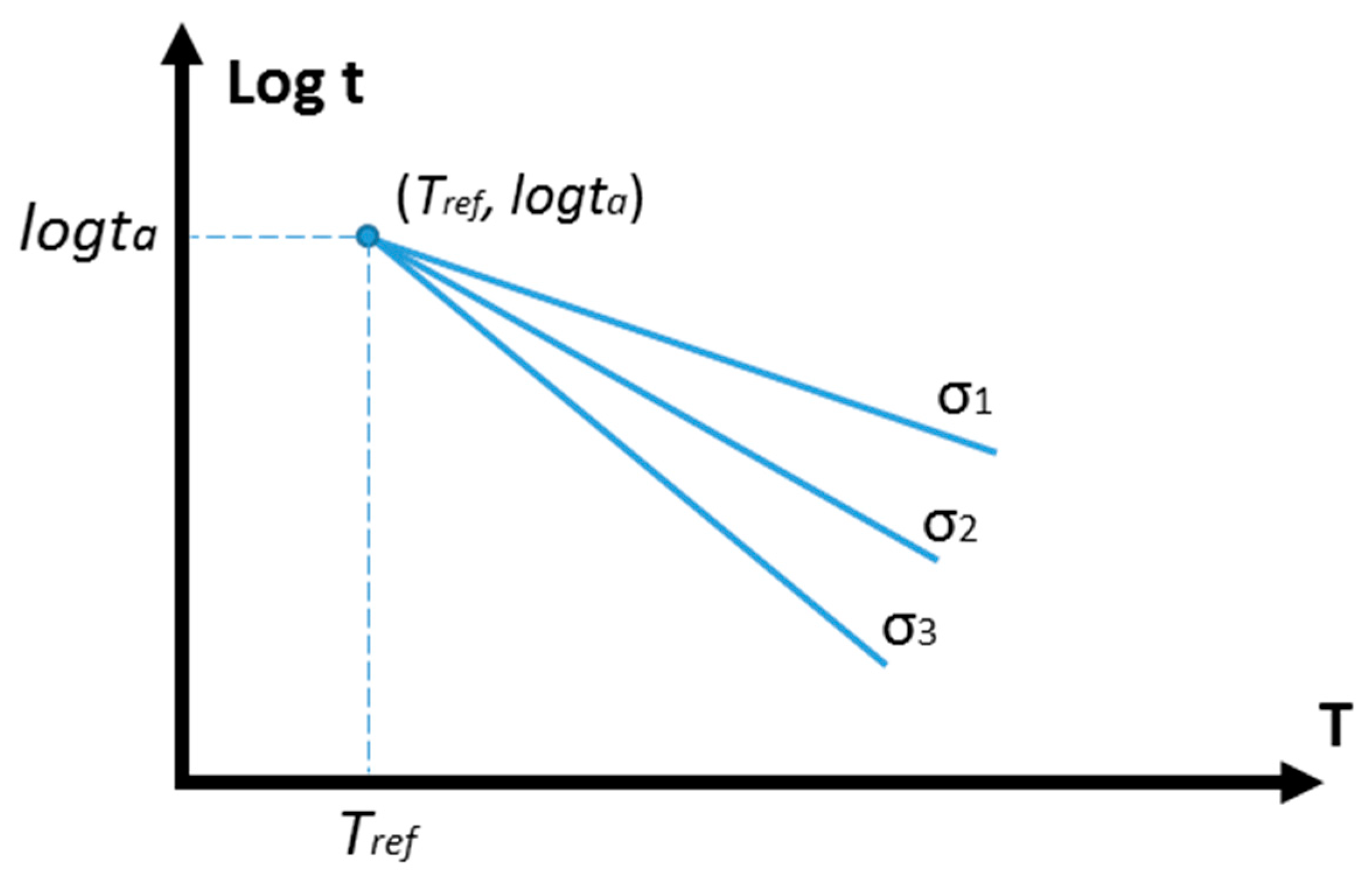
Both Equations (17) and (18) are obtained by the empirical data of pure creep. Specifically, during creep-rupture tests, the temperatures (T), stresses (σ) and creep-rupture times (t) are recorded. Then, the relationships between T and under different stresses are plotted (Figure 1), wherein the temperature at the point of convergence is identified as the reference temperature, and the value of at this convergence point () is given by the average value of the logt() at different stresses. The value of then gives .
According to Figure 1, the Manson–Haferd parameters under different stresses are given, then the relationship between the Manson–Haferd parameter and applied stress () can be obtained through curve fitting. Then, function is expanded.
3.2.3. Deriving the Coefficients
The remaining coefficients in the explicit model are determined by the empirical data of creep fatigue. Specifically, during the creep-fatigue tests, the temperatures (T), cyclic time (t), stresses (σ), plastic strain () and fatigue life (N) are recorded. In particular, with the empirical data of plastic strain vs. stress, the coefficients (K′ and n′) of the cyclic strain–stress relation under different temperature-cyclic time conditions are obtained. In the present work, these two coefficients are applied to describe the engineering quantities-based relationship, and a power-law-based transition between strain and stress is included. They then are involved in the function for transforming stress into plastic strain (Equation (20)), and a moderating factor () is introduced to compress the stress effect on creep-related damage. We did not separate the whole of applied loading () into two components. This is because we cannot say one part the applied loading contributes to creep, and another part contributes to fatigue. Therefore, we defined that the whole of applied loading works for both fatigue and creep damage.
In the present work, we define as a stress-moderating factor which is applied to compress the cyclic stress to an equivalent constant stress. This moderating factor is related to the shape of the loading wave, and presents the average level of the cyclic loading. Illustratively, the area below the contour of the cyclic loading along the time dimension should be equal to the area below the contour of the equivalent constant loading at the same time period. This is based on an assumption that creep makes the same contribution to tensile and compressional portions. Although this assumption may be not appropriate for some materials [33,34], it simplifies the method of extracting this factor. For example, is defined as 0.6366 for the sinusoidal wave and as 0.5 for the triangular wave.
Then, numerical optimisation was applied to derive the coefficients of , , and by minimizing the average difference () between the predicted fatigue life () and the experimental results () (Equation (21)).
where n is the number of data, and presents the fatigue life obtained at multiple conditions of (T, tc)j and strain amplitude i.
3.3. Evaluation of the Explicit Model
The quality of fatigue-life prediction is evaluated by the prediction ratio. Specifically, the prediction ratio (Equation (22)) gives the ratio of predicted creep-fatigue life to experimental creep-fatigue life:
In the present work, we define that:
An acceptable prediction ratio should be between 0.75 and 1.25.
This range is narrower (more conservative than the range shown in other literature, wherein a factor of 2 or 1.5 is normally given [25,35,36]. This also can be shown illustratively, where all data points of vs. under multiple temperatures and cyclic times should fall between the upper bound (+25%) and the lower bound (−25%) relative to ideal correlation (H = 1).
4. Validation
The explicit model is validated on the materials of 63Sn37Pb solder and stainless steel 316. The coefficients are determined by using the method proposed in Section 3.2, where the empirical data are extracted from the literature. The quality of fatigue-life prediction is evaluated by the method proposed in Section 3.3.
4.1. Validation on 63Sn37Pb Solder
4.1.1. Deriving the Coefficients
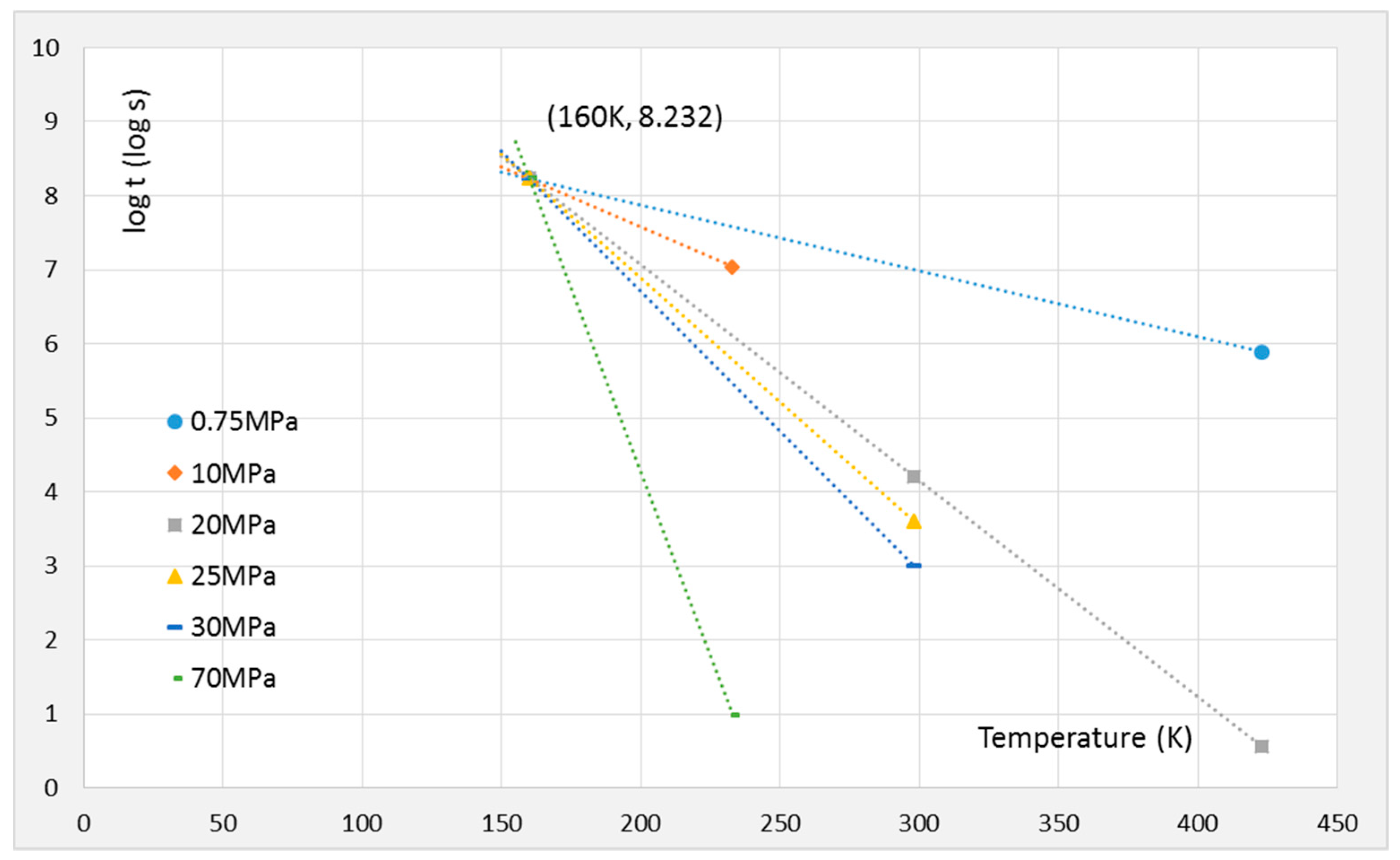
The reference temperature for 63Sn37Pb solder was chosen as 160 K and the reference cyclic time was defined as 1 s. The creep-rupture data [37] are plotted in Figure 2, and the point of convergence (, ) is evaluated as (160 K, 8.232). This gives
and the relationship between stress and the Manson–Haferd Parameter:
Then, substituting into Equation (24), function is expressed as:
and the magnitude of is given as 0.6366 for the sinusoidal wave.
The creep-fatigue coefficients [16] obtained from the literature are tabulated in Table 1. Minimizing the difference between the predicted creep-fatigue life () and the experimental creep-fatigue life () yields = 7.790, = 0.858, = 0.000234 and = 0.00596, and returns an average error () (Equation (21) of 0.000509.
Consequently, the coefficients of the explicit creep-fatigue equation for 63Sn37Pb solder are collected in Table 2:
4.1.2. Evaluation
To evaluate the explicit creep-fatigue model, another groups of creep-fatigue data (Table 3) [16] are used to compare with predicted fatigue life which is supported by the results shown in Section 4.1.1.
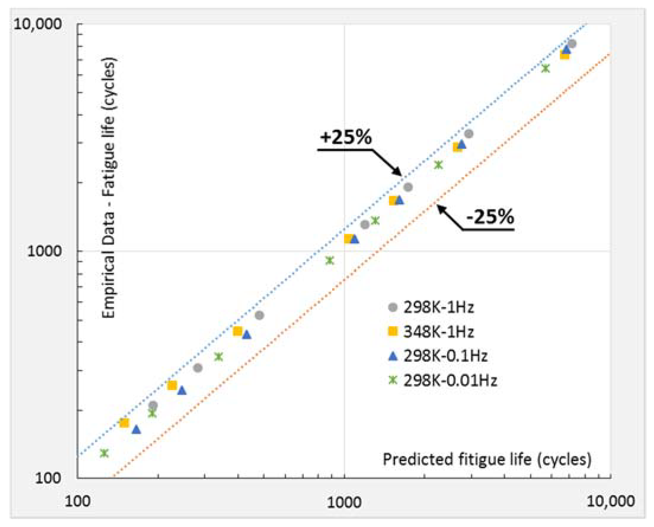
The prediction ratio (/) under multiple temperatures and cyclic times are plotted in Figure 3, where all data points fall between the upper bound (+25%) and the lower bound (−25%). The upper bound and the lower bound present the prediction ratios are 0.75 and 1.25 respectively. This implies that the explicit creep-fatigue equation provides a high quality of fatigue-life prediction, specifically, a relatively high correlation between predicted and experimental creep-fatigue life.
4.2. Validation on Stainless Steel 316
4.2.1. Deriving the Coefficients
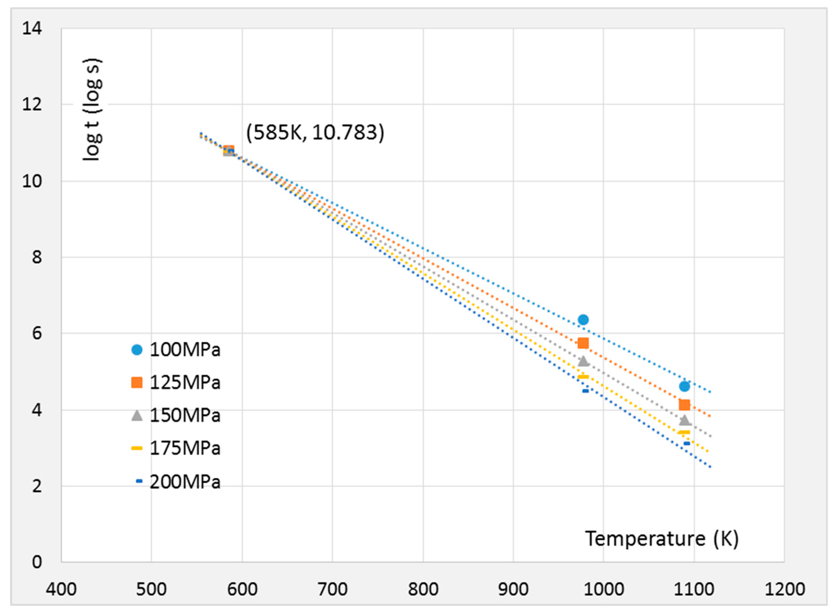
The reference temperature for stainless steel 316 was chosen as 585 K and the reference cyclic time was defined as 1 s. The creep-rupture data [38] are plotted in Figure 4, and the point of convergence (Tref, logta) is evaluated as (585 K, 10.783). This gives
and the relationship between stress and the Manson–Haferd Parameter:
Then, substituting into Equation (27), function is expressed as:
and the magnitude of is given as 0.5 for the triangular wave.
The creep-fatigue coefficients [39] obtained from the literature are tabulated in Table 4. Minimizing the difference between the predicted creep-fatigue life () and the experimental creep-fatigue life () yields = 7.768, = 0.571, = −0.000225 and = −0.0223, and returns an average error () (Equation (21)) of 0.00255.
Consequently, the coefficients of the explicit creep-fatigue equation for stainless steel 316 are collected in Table 5:
4.2.2. Evaluation
To evaluate the explicit creep-fatigue model, another groups of creep-fatigue data (Table 6) [39] are used to compare with predicted fatigue life which is supported by the results shown in Section 4.2.1.
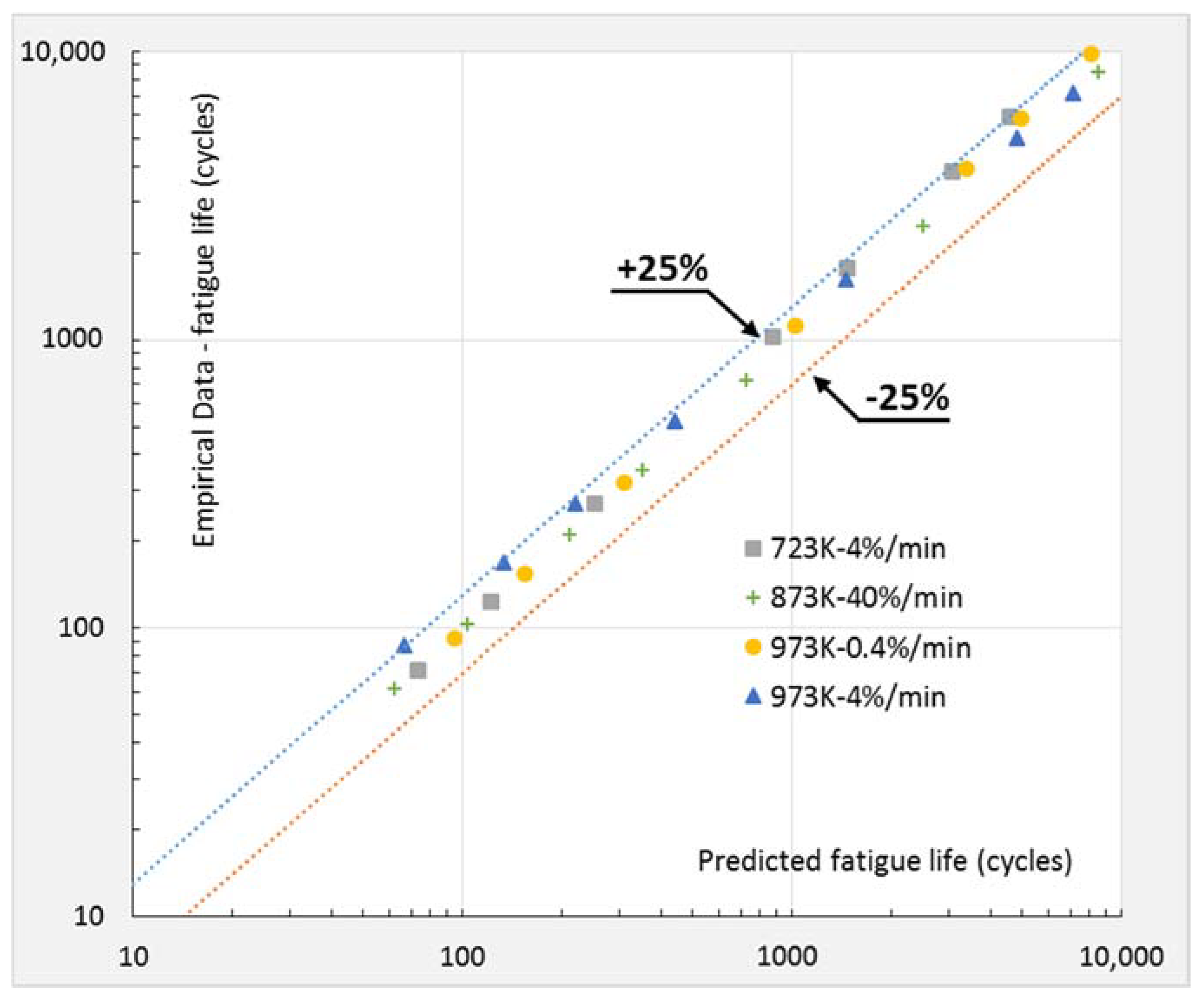
The prediction ratio (/) under multiple temperatures and cyclic times are plotted in Figure 5, where all data points fall between the upper bound (+25%) and the lower bound (−25%). The upper bound and the lower bound present the prediction ratios are 0.75 and 1.25 respectively. This implies that the explicit creep-fatigue equation provides a high quality of fatigue-life prediction, specifically, a relatively high correlation between predicted and experimental creep-fatigue life.
4.3. Accuracy Comparison: Explicit vs. Unified Models
The present work aims to improve the accuracy of the creep-fatigue-life prediction through further modifying the unified model. Thus, the ability of life prediction by applying the explicit model should be better than applying the unified model. This is proved through comparing the explicit model with the unified model on the materials of 63Sn37Pb and stainless steel 316.
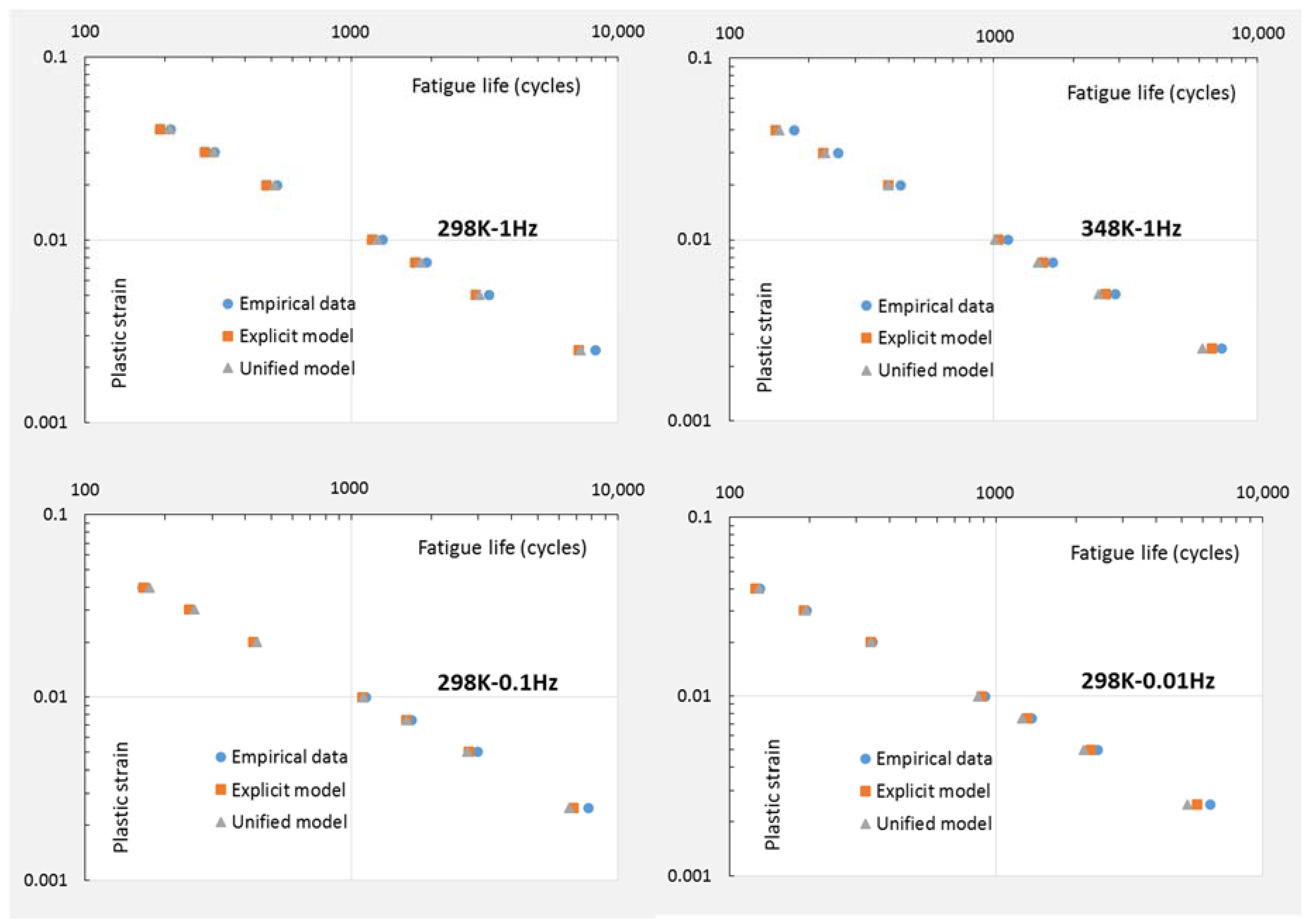
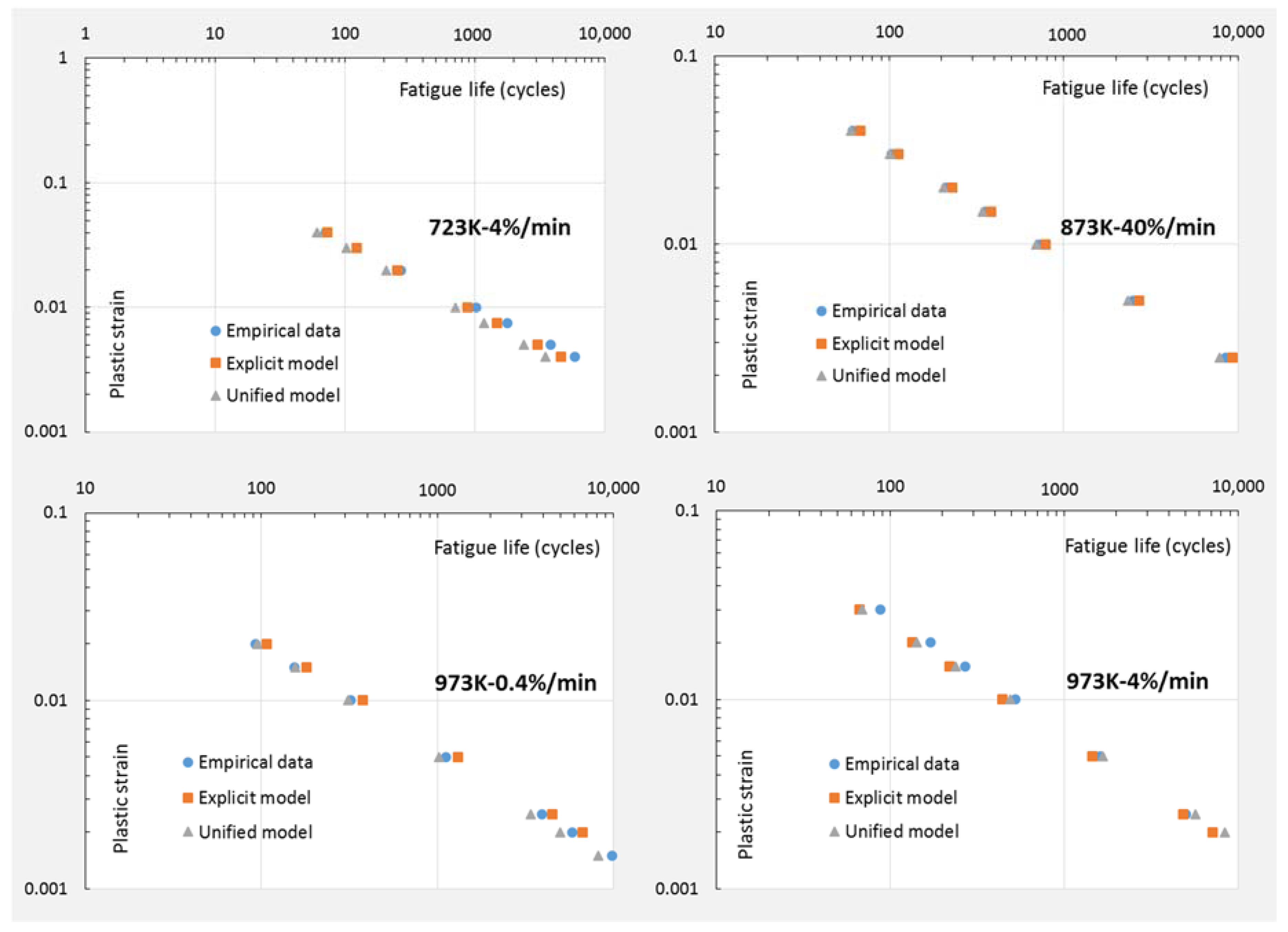
Specifically, the explicit formulation removes the assumption applied in the unified creep-fatigue model (Equation (2)), and then a creep moderating function was introduced into the exponent component. In this way, the explicit model has better ability to describe creep fatigue. To prove this, we applied the creep-fatigue data (Table 1 for 63Sn37Pb solder and Table 3 for stainless steel 316) to extract the coefficients of the unified model (Equation (2)) and the explicit model (Equation (15)). Then, these coefficients were applied to predict the fatigue life for the situations shown in Table 4 for 63Sn37Pb solder and Table 6 for stainless steel 316. The empirical data, and predicted life given by the unified model and the explicit model are illustrated in Figure 6 for 63Sn37Pb and Figure 7 for stainless steel 316.
Figure 7 and Figure 8 show that life-loading curves given by the explicit model are closer to the empirical data, thus we conclude that the explicit model has better ability to predict fatigue life at the creep-fatigue condition. This is also proved by the average errors and prediction ratios (see Equations (21) and (22) in Section 3.2.3 and Section 3.3 for the definitions of the average error and prediction ratio respectively) in Table 7. In particular, the value of the prediction ratio in Table 7 is represented by a range which is given by the maximum and minimum prediction ratios of the whole results. This representation is also shown in Table 8.
Table 7 shows that the explicit model provides smaller average errors and narrower ranges of prediction ratio for both the materials of 63Sn37Pb solder and stainless steel 316. This demonstrates that the explicit model has better accuracy for quantitatively representing creep fatigue.
4.4. The Ability to Describe Pure Fatigue
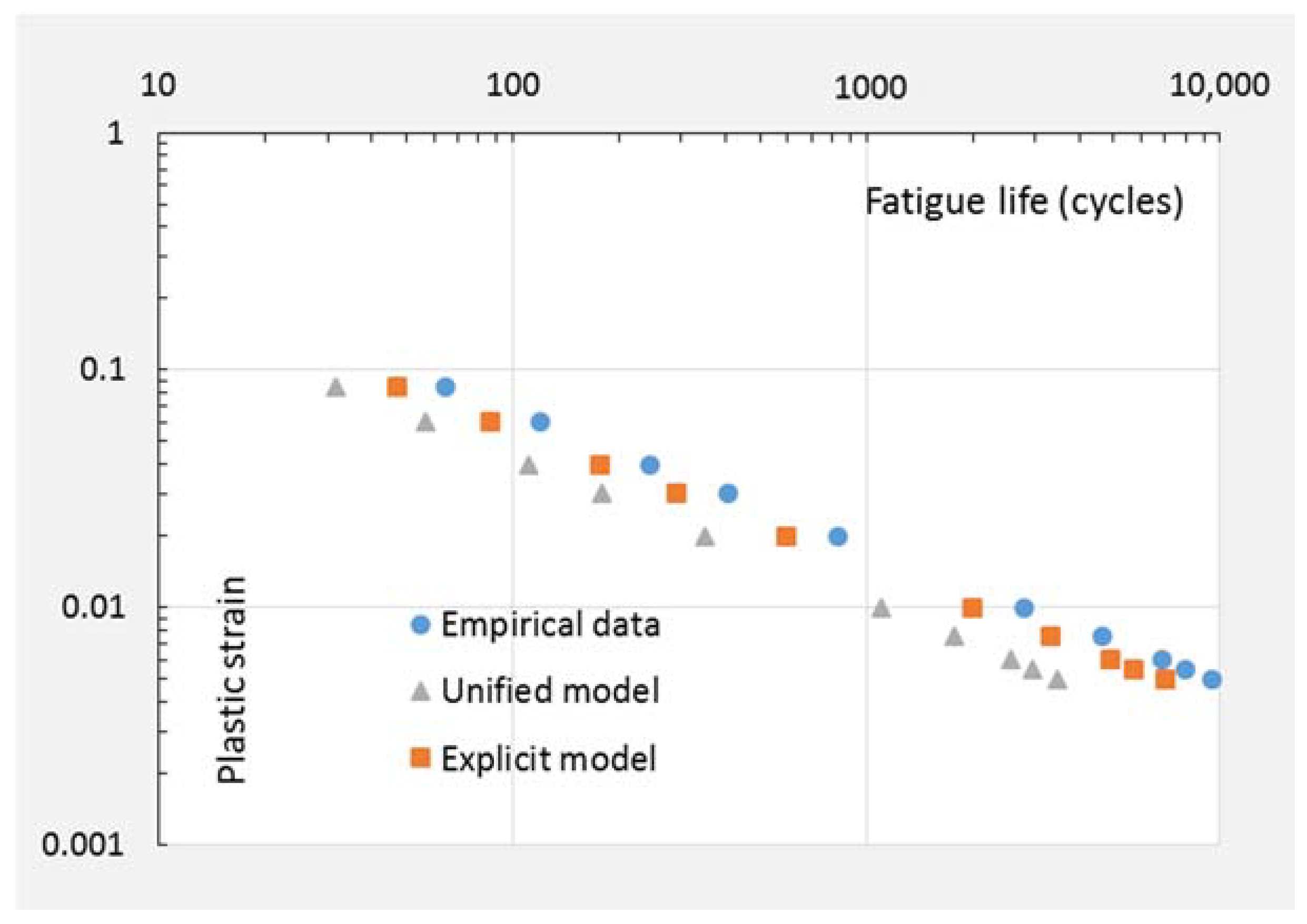
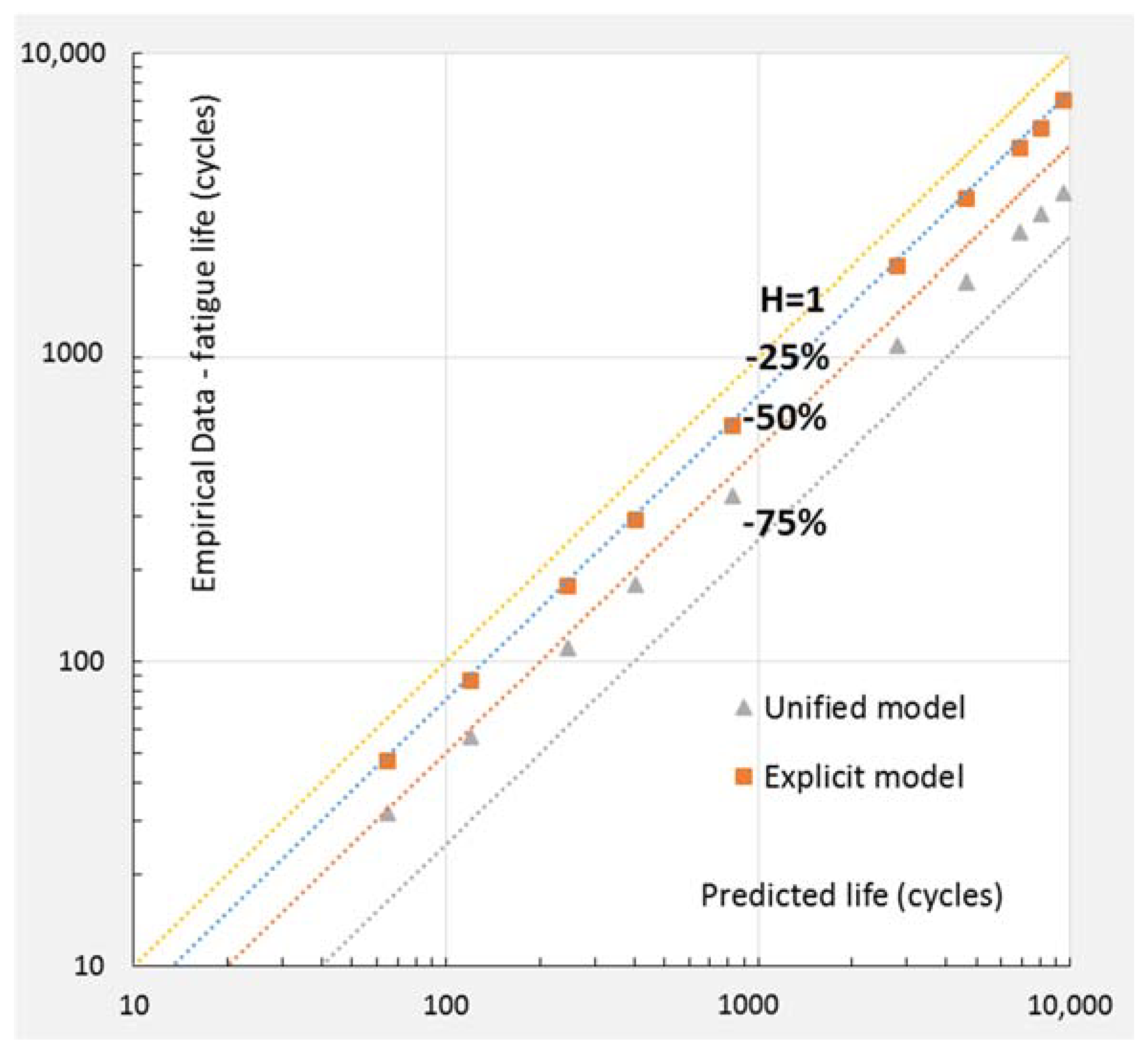
Both the unified creep-fatigue model and the explicit model can be restored into the Coffin–Manson equation at pure fatigue. This loading condition is numerically presented by the coefficients of and , thus the accuracy of pure-fatigue description is determined by them. In the present work, this ability was evaluated through comparing the predicted life with the empirical data on stainless steel 316 [39] (Figure 8).
Figure 8 shows that the loading-life curve formulated by the coefficients of and in the explicit model is closer than the unified model to the empirical data. This is also described by the prediction ratio. The prediction ratios for these two models is presented in Figure 9. The dotted lines (bounds) which are labeled by 1, −25%, −50% and −75% in Figure 9 represent the prediction ratios of 1, 0.75, 0.5 and 0.25 respectively.
Figure 9 shows that the pure-fatigue prediction ratios are around 0.75 for applying the coefficients of the explicit model, but the prediction ratios are lower, between 0.5 and 0.25, for using the coefficients of the unified model.
4.5. General Process of Validation for Other Materials
The explicit model could be further validated through involving more empirical data on more materials. The general process of validation can be summarised as follows:
(1) Obtain the empirical data for one specific material. The data include pure-creep data and creep-fatigue data, which could be extracted from the literature, or collected by performing testing. In particular, the creep-fatigue data under multiple temperatures and cyclic times are divided into two groups (3 to 4 sub-group data at different temperatures and cyclic times for each group). One group data (named Group1) are applied to determine the coefficients of the explicit model, and other group data (named Group2) are applied to compare with the predicted life (evaluate accuracy of the fatigue-life prediction).
(2) Determine the coefficients of the explicit model. The coefficients are determined by the method presented in Section 3.2.
(3) Predict fatigue life. With the coefficients obtained in step 2, the predicted life under the situations presented in ‘Group2’ are calculated through using the explicit model.
(4) Evaluate the explicit model. The evaluation of the explicit model is conducted by the method given in Section 3.3. This process is numerically and illustratively presented by the prediction ratios. If the predicted data satisfy the range of acceptation given in Section 3.3, we can conclude that the explicit model can be applied on this material to predict creep-fatigue life.
5. Discussion
5.1. The Characteristics of the Explicit Creep-Fatigue Model
The explicit creep-fatigue model was validated on the materials of 63Sn37Pb solder and stainless steel 316 (see Section 4). This implies that this model has ability to be applied at multiple temperatures and cyclic times, and the relationships between different variables (temperature, cyclic time, applied loading and life) in the explicit model are applicable for different materials.
In addition, at the reference (the pure-fatigue) condition (where and ), the explicit creep-fatigue model can be restored to the Coffin–Manson equation. At the pure-creep condition (where ), the explicit creep-fatigue model can be reformed as the Manson–Haferd parameter for creep. Consequently, the explicit formulation recovers both of the standard fatigue and creep formulations.
Consequently, the explicit model (Equations (15) and (16)) has the following features:
- Provides one formulation that covers the full range of conditions from pure fatigue, to creep fatigue, then to pure creep.
- Recovers the mathematical formulation of both of the standard fatigue and creep formulations (Coffin–Manson and Manson–Haferd respectively).
- Accommodates multiple temperatures. Specifically, the explicit model can be applied to predict fatigue life at situations with different temperatures.
- Accommodates multiple cyclic times. The explicit model is applied at the cyclic loading without hold time, thus the cyclic time refers to the period of one cycle of this loading condition. This is a limitation of this model, which will be discussed in Section 5.4.
- Accommodates multiple materials. The explicit model was not a purely empirical-based model because the physical meaning was indirectly introduced into the explicit model. This process is quite different from the curve-fitting method. Thus, we conclude that the explicit model is potential able to be applied for multiple materials: we have demonstrated validation for 63Sn37Pb solder and stainless steel 316. Further validation on different materials is needed: this will be discussed in Section 5.4.
- Provides a physical basis for the structure of the formulation. The basis of the term has been explained previously [40]. Specifically, diffusion-creep behaviour gives a linear relationship of temperature vs. loading and a logarithmical relationship of temperature vs. cyclic time. Plastic zone around the crack tip gives a power-law relation between life and loading. The new term is justified on principles of diffusion-creep rate and represents Fick’s law (see Section 3.1). Both and terms were built on the concept of fatigue capacity, which was formulated as ‘1 − x’. This formulation numerically presents the negative effect of creep on fatigue. In addition, the introduction of the reference condition gives an opportunity to connect pure fatigue with creep fatigue.
Attributes 1–2 may be considered ‘integrated’ attributes, 3–5 ‘unified’ attributes, and 6 a ‘natural origin’ attribute. Regarding integration, the models based on microstructural features, e.g., the integrated creep-fatigue theory [41,42], also offer an integrated characteristic. However, the determination of microstructural variables (such as crack, damage size and inter-void spacing) is challenging in the engineering situation. The explicit model is potentially easier to use in the engineer case.
Furthermore, the explicit model can be restored to the Coffin-Mason equation at pure fatigue and can be reformed as the Manson–Hefard parameter at pure creep. Both of these two formulations are conventional engineering models, and can be applied for engineering design without the need of observations at the microstructural level. This is a positive feature.
By natural origin we do not necessarily mean that the model has a physical basis traceable to microstructure and mechanical properties. Rather that the formulation of the model is consistent with existing representations of principles of physics (e.g., laws). We acknowledge that a full connection of all parameters in the explicit model to measureable variables of microstructure remains elusive. This limitation applies to all creep and fatigue models.
While there are other creep-fatigue formulations that also have high accuracy, they lack one or more of the features of the explicit model: they do not have the integrated characteristic; they are typically accurate only for specific cases (poor unified attribute); or they rely on the inclusion of many coefficients (typically into power series) which have no natural origin. Many of the competing models are so over-endowed with coefficients, e.g., [16,18], that they also have the risk of parameter non-identifiability.
5.2. The Ability to Describe Creep Fatigue
The unified model (Equation (2)) presents better ability to predict life at the creep-fatigue condition. This was proved through comparing the unified model with the existing creep-fatigue models. For example, the unified model was compared with Solomon’s model [15], Jing’s model [17], and Wong & Mai’s model [18].
Both Solomon’s model and Jing’s model use fixed coefficients. When they are applied to other situations, Solomon’s model results in a poor average error (23.96), and Jing’s model cannot give any numerical solution. Thus, they only can be used in the situations where they were derived, and cannot be extended to other situations and other materials where there are no empirical data. This is because these models determine their coefficients by numerical optimisation across all variables (including temperature, frequency, fatigue life and applied loading). Hence when changing to a different material it is necessary to recalculate all the coefficients: it is not possible to simply change only some of the coefficients. However, Wong & Mai’s model has potential to be applied to multiple materials. This is because this model has seven independent coefficients which are required to be recalculated for different materials. The accuracy of these models comes at the cost of high specificity of the coefficients, and the risk of parameter non-identifiability. Also, the coefficients in the power series terms have no physical identity, but only exist to provide improve mathematical fit.
To allow a comparison with the explicit model, we re-calculated the coefficients for Solomon’s model, Jing’s model, and Wong & Mai’s model, as follows.
Solomon’s model (Equation (29)) is:
with
where is temperature in °C, is the frequency, is the fatigue life, and , , , , and are constants derived from the empirical data.
Jing’s model (Equation (31)) is:
with
where , , , , and are constant derived from the empirical data.
Wong & Mai’s model (Equation (33)) is:
with
where is cyclic hardening index, is the yield stress, is the temperature in Kelvin, is the frequency, is the reference temperature below which creep becomes dormant, is the reference frequency, and , , , , , and are constant.
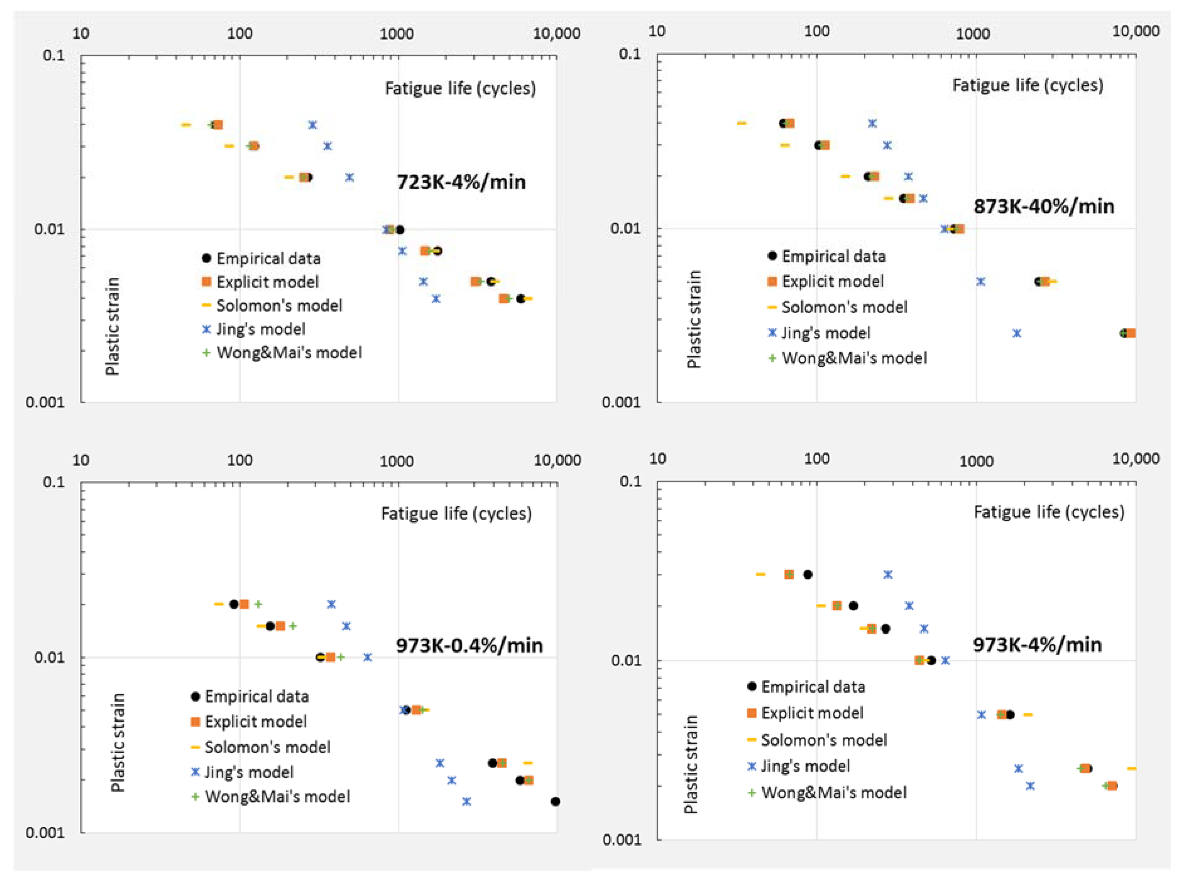
We recalculated all these constants, for these three models, for stainless steel 316, and plotted the results in Figure 10 to compare with the explicit model and empirical data.
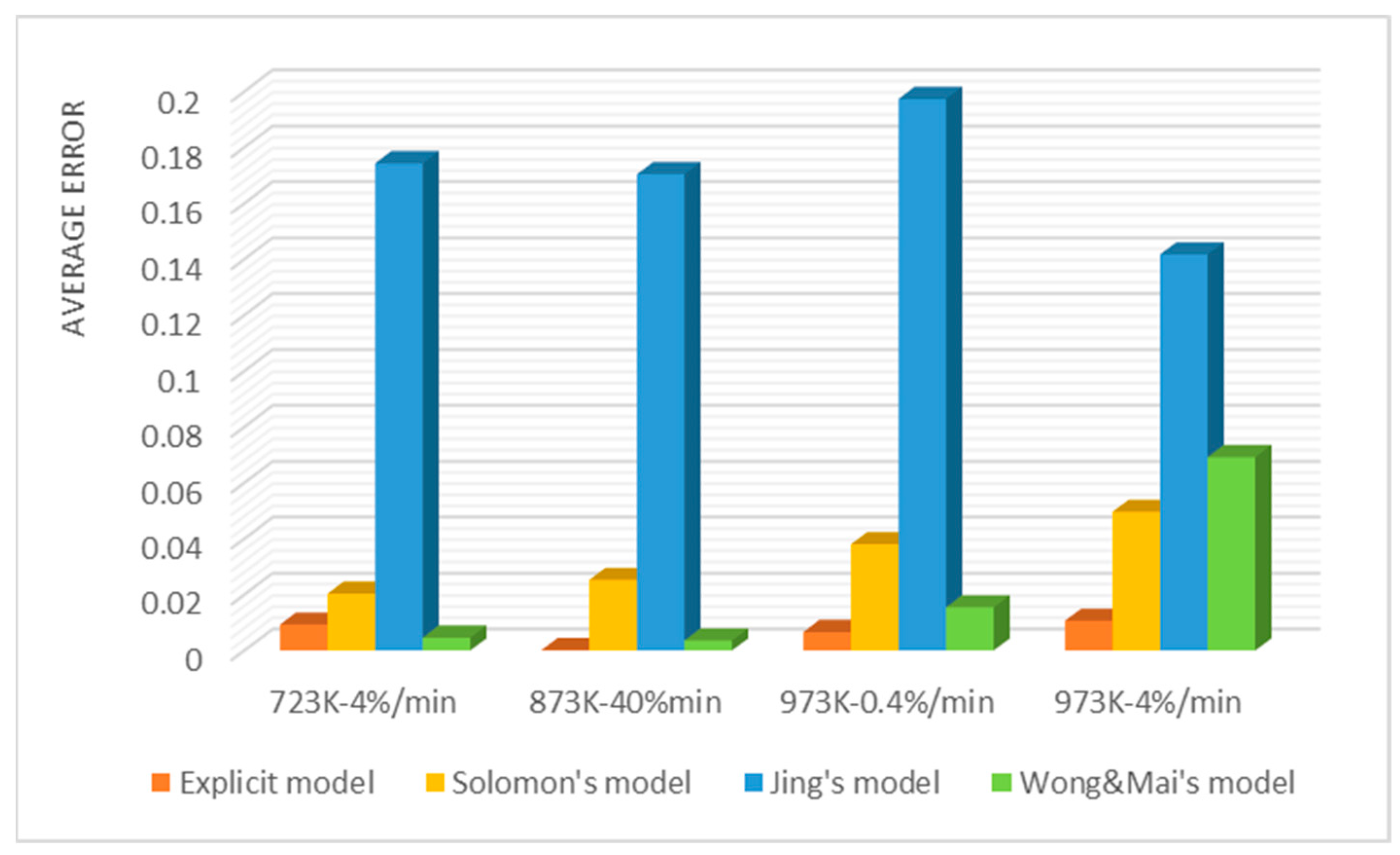
The average errors calculated by Equation (21), for the explicit model, Solomon’s model, Jing’s model, and Wong & Mai’s model, for stainless steel 316, are plotted in Figure 11:
Both Figure 10 and Figure 11 show that the explicit model (Equation (15)) has better numerical accuracy for describing creep fatigue than the models of Solomon, Jing, and Wong & Mai models. For Solomon’s and Jing’s models, the average error given by these two models are much higher than the explicit model. This is because the relationships between different variables in these two models were completely derived from the empirical data of one specific material, thus they cannot be extended to other materials. However, Wong & Mai’s model presents better ability for life prediction than Solomon’s and Jing’s models (except the situation of 973 K-4%/min). This may be because Wong & Mai’s model involves a material property (yield stress), and it also applied a concept that would later be referred to as fatigue capacity. However, this model has seven independent coefficients which are required to be determined by empirical data. Consequently, this leads to another issue, that of economy.
5.3. The Economy
The economy is an important factor which is considered during the process of engineering design [4]. An economical method should provide a good balance between the accuracy and cost. Although the mechanism-based models may not need any creep-fatigue tests, observing and measuring microstructure is not a simple and economic process for engineering practitioners. The empirical-based models are more suited for engineering purposes, hence are the point of comparison for the explicit model. We selected Wong & Mai’s equation [18] to compare with the explicit model regarding to the economy, since the Wong & Mai’s equation shows better life-prediction ability than other existing models (see Section 5.2).
In the present work, empirical data under different temperatures and cyclic times was taken from the literature (Table 4). The first stage took seven groups of data and split this into a group of six and one. The six groups of empirical data were applied to derive the coefficients of Wong & Mai’s equation and the explicit model. Then, these coefficients were used to predict fatigue life at the condition of the remaining data set (named ‘predicted condition’). The discrepancy was noted.
The second stage repeated this analysis but with three and four groups respectively, and again the discrepancy was noted. Finally, the average errors and prediction ratios obtained in these two situations were compared. Thus, it becomes possible to infer how sensitive each model is to the available quantity of data. A model with better economy would be one where the degradation in accuracy was less sensitive to the quantity of data.
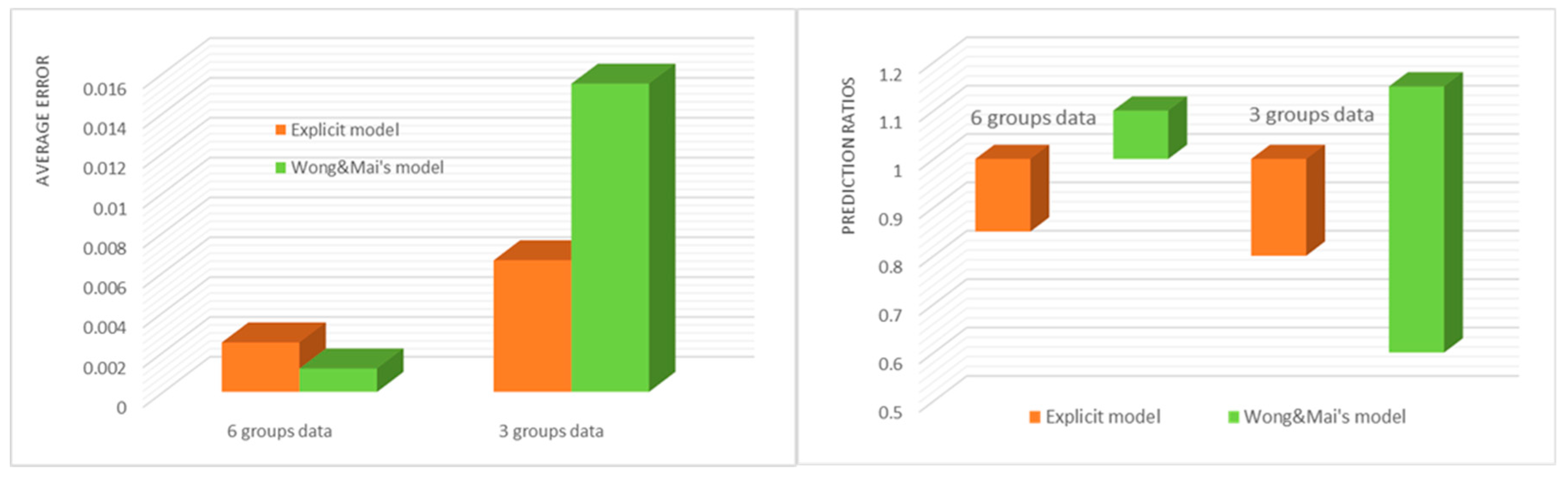
The comparison between Wong & Mai’s equation [18] and the explicit model for the accuracy of the fatigue-life prediction regarding the empirical-data number is shown in Table 8 and Figure 12 for stainless steel 316.
Table 8 and Figure 12 show that the Wong & Mai equation gives better accuracy for the fatigue-life prediction (at the condition of 973 K-0.4%/min) than the explicit model when six groups of creep-fatigue data are available. This is because the Wong & Mai equation has more independent coefficients which are extracted through the numerical optimisation (a curve-fitting-based method), which results in a better fitting quality when enough empirical data are involved [43].
When only three groups of creep-fatigue data were selected to obtain the coefficients, then the situation changes. The Wong & Mai equation experiences more severe degradation against both measures: average error and prediction ratio.
In both cases the numerical optimization still yields quite small average errors for fitting for the Wong & Mai equation. However, poor accuracy results when Wong & Mai’s equation with the coefficients obtained at this stage is extended to predict fatigue life at the ‘predicted condition’ (973 K-0.4%/min). Specifically, for the Wong & Mai equation, the average error worsens from 0.001176 to 0.01547, and the range of prediction ratio also widens.
The explicit model also degrades, but not to the same extent. Specifically, the average error is 0.002481 for the coefficients obtained from six groups of creep-fatigue data, and 0.006608 for the coefficients obtained from three groups of data. Meanwhile, the range of prediction ratio only slightly changes between these two situations.
Thus, the explicit model shows greater robustness for smaller datasets. This is significant is it indicates that fewer creep-fatigue experiments are necessary to obtain the coefficients of the explicit model. As a result, we conclude that the explicit model is the more economical method because less empirical data are required.
The explicit model was developed through introducing the parameters of temperature and cyclic time into the exponent component, and thus two more coefficients ( and ) were included. This leads to a risk that more empirical data are required to obtain high-fitting accuracy. However, Table 8 implies this risk is not significant. Although the accuracy is reduced if less empirical data are applied to determine the coefficients, the difference of errors between these two situations is small based on a log-scale calculation, and the reduced accuracy still provides good ability for life prediction (this was proved in Section 4).
We suggest that the robustness of the explicit model arises because the parameters and corresponding coefficients were introduced into the exponent component (modifying the fatigue ductility exponent) rather than the coefficient component (modifying the fatigue ductility coefficient). In this case, the process of numerical optimisation for the coefficient and exponent components was conducted in two relatively separate directions. While this reduced the accuracy somewhat, it also reduced the risk of parameter non-identifiability. We expect that the economy would worsen if the modification was conducted for the coefficient component, since this already has a several tunable coefficients.
Consequently, we conclude that the explicit creep-fatigue model presents an economical method for the fatigue-life prediction, and introducing two more coefficients into the exponent component does not significantly impact the economy.
5.4. Limitations and Implications for Future Research
Limitations that designers need to note are that strictly speaking the method has only been validated for the materials of 63Sn37Pb and stainless steel 316. However, this explicit model is potentially usable for other metallic materials. We anticipate difficulties applying this model for plastics and composites because they present totally different material characteristics and failure mechanisms. However, it is not impossible that this explicit model may be further improved and extended to other material categories as more empirical data are included. In particular, nylon is widely used in the engineering industry for load bearing parts. Thus, it may be an interesting future project to check and adapt this model to engineering nylon (such as nylon 6).
The explicit model is not yet ideal regarding natural origin as it does not include quantifiable microstructural properties. To achieve this, it would be necessary to better understand the microstructural processes of fatigue & creep—especially their interactions—and how those affect plastic strain and life. Some work is available in this area, e.g., [24], but there is still a long way to go before the values of coefficients in a creep-fatigue model can be predicted ab initio from microstructural inspection. In addition, as mentioned in Section 2, the explicit model ignores the dislocation creep and grain boundary sliding. In this case, introducing these two behaviours to reflect creep effect at high stress may be beneficial.
Another potential avenue of future research is to continue the process of extending existing models towards a more complete theory, as has been illustrated here with the redevelopment of the unified model into the explicit. During the process of development, more microstructural-level-based parameters may be included, with a corresponding inclusion of new terms into the model. We suggest that it is worthwhile designing these extensions to include other well-established phenomena, as we demonstrated in Section 3, rather than merely chasing better accuracy by adding more power terms and coefficients.
The situation of cyclic loading without hold time (dwell-fatigue) is not covered by the explicit model. In this loading condition, fatigue makes more of a contribution than creep, because the total time is too small to produce marked creep damage. However, for cyclic loading with hold time, the creep effect gradually intensifies as the hold time increases. Then more creep damage is produced than fatigue damage, and the failure finally occurs due to the creep effect. We could imagine that in the situation with a relatively short hold time, the explicit model may still present a reasonable prediction of fatigue life, but the accuracy of this prediction may become worse when the hold time is prolonged. This implies that the explicit formulation has an opportunity to be further improved to cover the situation with hold time or relatively long cyclic time. To achieve this, it would seem necessary to modify the formulation (especially, the creep component in this explicit model) to include new terms of as yet-unknown mathematical form. Conceptual works, e.g., [24], may be useful in identifying the basic form of these relationships.
At elevated temperature, the crack surface is oxidized, and then the material becomes more brittle. This results in further crack propagation. Therefore, the oxidation effect should ideally be included. The class of models based on observation of microstructure, e.g., [41,42], are superior in this regard because they can measure the voids and internal damage.
The class of models based on macroscopic empirical testing, to which the explicit model belongs, lack the microstructural parameters of crack length, oxidation, etc. At least not as primary variables, but the effects are partly accommodated through other means. In the explicit model, the coefficients are determined from the empirical data through numerical optimization, thus any oxidation effects are incorporated into the fitting process. Although the accuracy of fatigue-life prediction may be impacted, the results still show acceptable accuracy (see Section 4.3 and Section 5.2).
In future work it might be possible to include oxidization in the explicit equation. Superficially this might involve simply including a power series term. However this may not be entirely successful, because our observation is that simply adding more terms and coefficients does improve accuracy, but at the cost of introducing model degeneracy. This has the further consequence of making the model more highly dependent on the specific situation, i.e., reduces the ability of the model to generalize to other materials and situations. The challenge is to include the oxidation effect, in a way that is coherent with how the effect operates physically, and to do so using parameters that are identifiable by the engineering designer. This opens an opportunity to further improve this engineering-based model.
5.5. Application to Engineering Design and Structural Mechanics
The present work aims to develop a creep-fatigue model for engineering design, thus this section is included to briefly explain how this model is applied by manual engineering calculations and finite element analysis at the engineering design process.
Fundamentally, the explicit creep-fatigue model can be used to predict fatigue life at a given applied loading, or can be used to evaluate the critical value of applied loading under a given life. This process of engineering calculation is normally applied at the initial stage of engineering design. For example, the explicit model can be applied to select a material.
In addition, the explicit model can also represent the pure fatigue condition. This is because it can be restored to the Coffin–Manson equation at the reference condition ( and ), which represents pure fatigue wherein the creep effect is dormant. In this case, this restored equation can be used to predict the fatigue life or critical value of applied loading at pure fatigue. The accuracy of pure-fatigue description was demonstrated in Section 5.3, which implies the coefficients of and obtained in creep fatigue can be extended to predict fatigue life at pure fatigue.
The method may be applied to manual calculation or finite element analysis, as shown in Appendix A.
6. Conclusions
The present work modified the unified creep-fatigue model by introducing the parameters of temperature and cyclic time into the exponent component. In this way, the accuracy of the fatigue-life prediction for both the creep-fatigue and pure-fatigue conditions are improved. The explicit model has the following beneficial attributes: Integration—it provides one formulation that covers the full range of conditions from pure fatigue, to creep fatigue, then to pure creep. The inclusion of the reference condition gives an opportunity to connect pure fatigue with creep fatigue. It also recovers the mathematical formulation of both of the standard fatigue and creep formulations (Coffin–Manson and Manson–Haferd respectively); Unified—it accommodates multiple temperatures, multiple cyclic times, and multiple metallic materials; Natural origin—it provides a physical basis for the structure of the formulation, in its consistency with diffusion-creep behaviour, the plastic zone around the crack tip, and fatigue capacity; Economy—although two more coefficients were introduced into the explicit model, the economy is not significantly impacted; Applicability—the explicit model is applicable to engineering design. This was demonstrated by its application to manual engineering calculations, and also to finite element analysis.
The overall contribution is that the explicit model provides improved ability to predict fatigue life for both the creep-fatigue and pure-fatigue conditions.
Author Contributions
The explicit model was developed and validated by D.L., the discussion and application of this new model were conducted by D.L. and D.J.P.
Funding
This research received no external funding.
Conflicts of Interest
The authors declare no conflict of interest. The research was conducted without personal financial benefit from any funding body, and no such body influenced the execution of the work.
Nomenclature
| cross-sectional area | |
| constant | |
| , , , and | constants |
| fatigue ductility coefficient | |
| , , , , and | constants |
| diffusion coefficient | |
| amount of substance flowing through a unit area | |
| Young’s modulus under consideration | |
| applied force | |
| frequency of applied force cycles | |
| stress moderating factor | |
| reference frequency | |
| Gibbs free energy for formation of a vacancy | |
| prediction ratio | |
| diffusion flux | |
| cyclic strength coefficient | |
| K | Boltzmann’s constant |
| surface condition modification factor | |
| size modification factor | |
| load modification factor | |
| temperature modification factor | |
| reliability factor | |
| miscellaneous-effects modification factor | |
| length | |
| change of the length | |
| experimental results of fatigue life | |
| creep-fatigue life | |
| predicted fatigue life | |
| equilibrium atomic fraction of vacancies | |
| n | number of data |
| cyclic strain hardening exponent | |
| Manson–Haferd parameter | |
| endurance limit | |
| rotary-beam test specimen endurance limit | |
| temperature | |
| reference temperature | |
| t | creep-rupture time |
| cyclic time | |
| reference cyclic time | |
| position | |
| fatigue ductility exponent | |
| average difference | |
| elastic strain | |
| plastic strain which reflects fatigue capacity | |
| total strain | |
| applied loading | |
| yield stress | |
| concentration of vacancies | |
| atomic volume | |
| creep moderating function | |
| temperature moderating function | |
| cyclic time moderating function | |
| stress moderating equation | |
| stress function | |
| (, ) | point of convergence of the -T lines |
Appendix A. Application for Engineering Design
Appendix A.1. Manual Calculation Method for Design
The design engineer needs to determine the coefficients of the explicit equation for the material of interest. This is achieved by the following steps:
(a) Obtain empirical data for the material of interest. The data needed are pure creep, and creep fatigue. The pure creep data are generally commonly available in the literature, and if not then the empirical test is not onerous. The creep-fatigue data may also exist, but if not then a more extensive testing regime is necessary. This is where the economy of the explicit model is advantageous. In particular, in this process of creep-fatigue testing, the cyclic strength coefficients (K′) and cyclic strain hardening exponents (n′) under different temperatures and cyclic times are extracted. Then, the parameters of cyclic strain-stress relation (K′ and n′) are formulated in functions of temperature and cyclic time ( and ) through curving fitting. This is conventional practice; see Equation (19).
(b) Extract the coefficients of the explicit model using the method shown in Section 3.2. This process involves numerical optimisation, which may be achieved by using a spreadsheet (e.g., MS Excel® 2013) or other solver. Numerical optimisation is applied to determine the coefficients of , , and by minimizing the average difference () (Equation (21)).
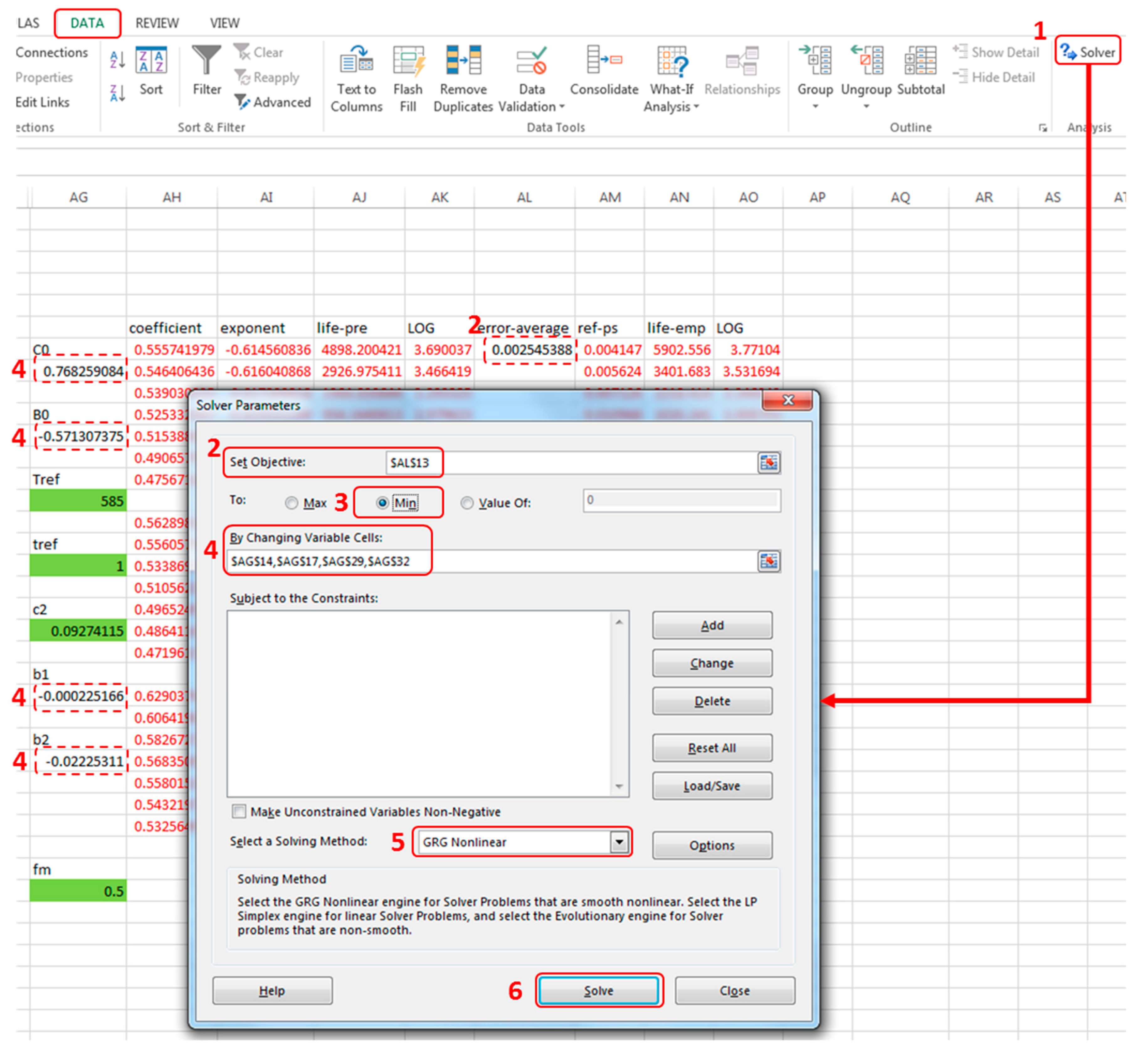
This method involves the following six steps and is shown in Figure A1:
- Opening Excel® solver: DATA → Solver
- Selecting objective: selecting optimum cell in the spreadsheet. In the present work, the cell which shows average error is selected.
- Defining optimized condition: defining the criterion of numerical optimization for the value of the optimum cell. In the present work, the option of ‘Min’ is selected to find the minimum average error.
- Selecting variables: selecting adjustable cells in the spreadsheet. In the present work, the cells which give the values of , , and are selected.
- Selecting solving method: selecting the numerical optimization algorithm. In the present work, we select the method of ‘GRG Nonlinear’ which is applied to the smooth-nonlinear situation.
- Clicking ‘Solve’ to get results.
After this, designers get all the coefficients of the explicit equation. Then this equation can be applied to predict fatigue life under consideration. This is conducted by the following steps:
(c) Determine loading conditions. They are force (F), temperature (T) and cyclic time (t). These will be known, or able to be estimated, by the designer.
(d) Determine plastic strain in the geometry under consideration. The plastic strain is determined by a stress-centric approach (Equation (A1)):
where is the total strain, is the elastic strain, is the length, is the change of the length, is the applied stress, is the Young’s modulus under consideration, is the applied force, and is the cross-sectional area.
(e) Calculate fatigue life. With the cyclic strain-stress relation extracted in step (a), the coefficients obtained in step (b), and the values of temperature, cyclic time and plastic strain given by steps (c) and (d), the fatigue life is calculated by Equation (A2):
Overall, we conclude that this simple process can readily be used to provide a more detailed and accurate representation of life under creep-fatigue conditions.
Figure A1.
Spreadsheet method for numerical optimization, using Excel®.

Appendix A.2 Using the Explicit Equation for Finite Element Analysis (FEA)
The conventional method for creep-fatigue in FEA is for the algorithms to determine the plastic strain in the part, based on the stress and the pure creep loading (strain dependency on applied temperature). The Coffin–Manson equation (Equation (A3)) is then used to determine the life.
where is the plastic strain amplitude, is the fatigue ductility coefficient and c is the fatigue ductility exponent.
Conventional finite element creep-fatigue simulation is conducted under cyclic loading and elevated temperature. Generally, this is a complex process. There are two areas where the explicit equation simplifies the process.
First, the conventional FEA process requires empirical data for the specific loading case. This comprises a creep test (strain vs. time) for the applied loading. The creep parameters are determined using curve-fitting, and input to software. There is a need to redo the creep test when the applied loading is changed. In contrast the explicit method has the following advantages: (a) It merely requires data from a creep rupture test—this is a simpler test to perform; (b) If the loading changes, say due to modifications in the design conditions (geometry, temperature, stress, etc.), then there is no need to perform another empirical test nor to recalculate the coefficients. The explicit equation already includes all the variables for multiple different loading conditions.
Second, the conventional FEA process treats the creep effect as independent to the fatigue induced strain. Consequently this may result in non-convergence for FEA, and then the analysis settings may need to be repeatedly modified to attempt convergence. In contrast the explicit method has the advantage of removing the creep parameters. The creep strain is instead included in an integrated manner with the fatigue formulation. Consequently non-convergence is less of an issue.
The benefits of the explicit model is that it provides a method for representing the interaction between creep and fatigue. Thus, the creep effect may be removed from the simulation and the simpler process of creep-fatigue life prediction can be applied. Ideally the explicit model would be formulated within the FEA software, but this is not currently the case. However there is a way to circumvent this problem, which involves adapting the coefficients of the Coffin–Manson equation to represent the full creep-fatigue behaviour. We illustrate this using ANSYS® 17.0 (ANSYS, Inc., Canonsburg, PA, USA). We do not show the other parts of the FEA workflow, such as the setting up of the model and the convergence as we assume the analyst will be familiar with those.
The process is as follows:
- (a)
- Obtain empirical data for the material of interest. See step (a) in Appendix A.1.
- (b)
- Extract the coefficients using the method shown in Section 3.2. See step (b) in Appendix A.1.
- (c)
- Determine loading conditions. They are stress, temperature and cyclic time.
- (d)
- Determine parameters imported into ANSYS® as engineering data. These parameters include the general material properties (such as yield stress, Young’s modulus and Poisson’s ratio) and the strain-life parameters under consideration. The general material properties are commonly available in the design handbook. The strain-life parameters are determined by the following method:The ductility coefficient () and ductility exponent () of the Coffin–Manson equation are given by the coefficient component () and the exponent component () of the explicit equation respectively.The cyclic strength coefficient () and cyclic strain hardening exponent () under consideration are determined by the relation obtained in step (a).The strength coefficient () and strength hardening exponent () are given by the compatibility equations (Equations (A4) and (A5)):
- (e)
- Operate FEA. In this process, the thermal effect is removed and the finite element simulation is performed under the pure-fatigue condition. Finally, FEA gives the fatigue life.
Note that this method may only be applied to evaluate the creep-fatigue life of the part. Specifically, the resulting stress/strain distribution and deformation shown by the FEA is unreliable, because its algorithms will not have modelled the creep effect. Nonetheless we believe the life prediction should be robust. However, this opens an opportunity for future research, where the combination between the explicit model and FEA may be further improved.
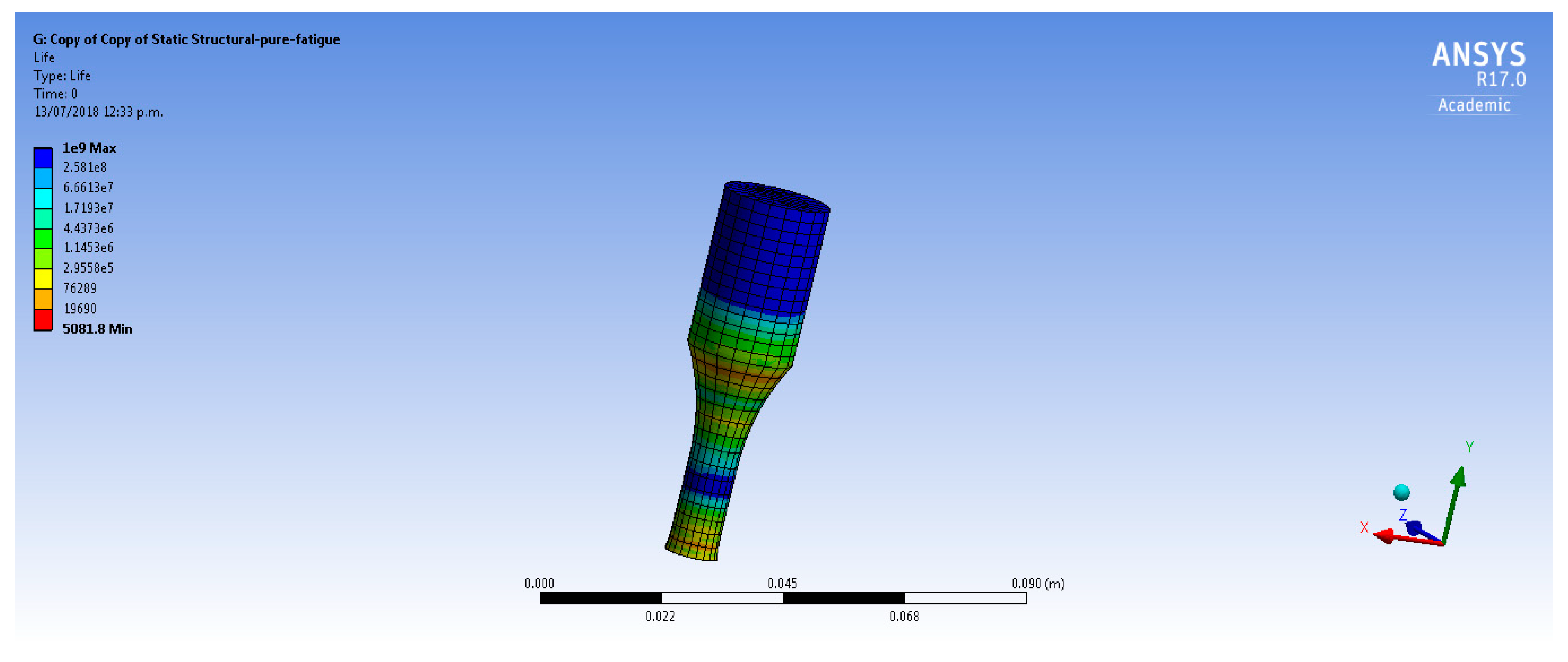
The accuracy of life prediction using the method above is demonstrated by the following example. In this example, we evaluated the fatigue life for a cylindrical specimen by two different FEA processes. On the one hand, we conducted simulation with creep effect and thermal condition. During this process, creep-related parameters were included as the engineering data, and the simulation was operated under cyclic loading at elevated temperature.
On the other hand, we conducted simulation using the explicit model (using the method above). In this process, the coefficient and exponent of the explicit model were imported into ANSYS® (Revision 17.0) as the fatigue parameters in engineering data. Since they already contain the creep effect, the creep-related parameters and thermal condition are removed from FEA. The fatigue life given by these two methods are shown in Figure A2 and Figure A3.
Figure A2.
Fatigue life obtained at the creep-fatigue condition using conventional method.

Figure A3.
Fatigue life obtained at the pure-fatigue condition using explicit method.

This example is also summarised in Table A1.

Table A1.
Fatigue evaluation by FEA.
| Simulation Using Conventional FEA Methods | Simulation Using Explicit Method | |
|---|---|---|
| Temperature | 977 K | 977 K but model parameters set to room temperature |
| Loading amplitude | 100 MPa | 100 MPa |
| Creep parameters | Were imported | Were removed |
| Mechanical properties | Values at pure fatigue | Values at the running condition |
| Fatigue parameters | Parameters at pure fatigue | Parameters were obtained from the explicit model at the running condition |
| Fatigue life | 5257 | 5081 |
Table A1 shows that these two life-evaluation processes give similar results (fatigue life), with the explicit method being slightly more conservative. The explicit method is faster to implement even for a single pass through the design, and has further time advantages when there are revisions and loops in the design process. We conclude that combining the explicit model with FEA can reduce the difficulty and complexity of analysis regarding fatigue evaluation, and speed up the design process. These benefits are particularly attractive early design stages, when the design is still experimental and the loading conditions are not finalized.
References
- Dowling, N.E. Mechanical Behavior of Materials: Engineering Methods for Deformation, Fracture, and Fatigue; Pearson: London, UK, 2012; p. 954. [Google Scholar]
- Chowdhury, P.; Sehitoglu, H. Mechanisms of fatigue crack growth—A critical digest of theoretical developments. Fatigue Fract. Eng. Mater. Struct. 2016, 39, 652–674. [Google Scholar] [CrossRef]
- Marin, J. Mechanical Behavior of Engineering Materials; Prentice Hall: Upper Saddle River, NJ, USA, 1962. [Google Scholar]
- Joseph Edward Shigley, C.R.M. Mechanical Engineering Design; McGraw-Hill Education: New York, NY, USA, 2001; p. 1248. [Google Scholar]
- Taira, S. Lifetime of structures subjected to varying load and temperature. In Creep in Structures; Springer: Berlin/Heidelberg, Germany, 1962; pp. 96–124. [Google Scholar]
- Ainsworth, R.; Ruggles, M.; Takahashi, Y. Flaw assessment procedure for high-temperature reactor components. J. Press. Vessel Technol. 1992, 114, 166–170. [Google Scholar] [CrossRef]
- Grell, W.; Niggeler, G.; Groskreutz, M.; Laz, P. Evaluation of creep damage accumulation models: Considerations of stepped testing and highly stressed volume. Fatigue Fract. Eng. Mater. Struct. 2007, 30, 689–697. [Google Scholar] [CrossRef]
- Pavlou, D. Creep life prediction under stepwise constant uniaxial stress and temperature conditions. Eng. Struct. 2001, 23, 656–662. [Google Scholar] [CrossRef]
- Lv, Z.; Huang, H.-Z.; Zhu, S.-P.; Gao, H.; Zuo, F. A modified nonlinear fatigue damage accumulation model. Int. J. Damage Mech. 2015, 24, 168–181. [Google Scholar] [CrossRef]
- Shang, D.-G.; Yao, W.-X. A nonlinear damage cumulative model for uniaxial fatigue. Int. J. Fatigue 1999, 21, 187–194. [Google Scholar] [CrossRef]
- Basquin, O. The exponential law of endurance tests. Am. Soc. Test. Mater. 1910, 10, 625–630. [Google Scholar]
- Wöhler, A. Theorie rechteckiger eiserner brückenbalken mit gitterwänden und mit blechwänden. Z. für Bauwesen 1855, 5, 121–166. [Google Scholar]
- Coffin, L.F., Jr. A Study of the Effects of Cyclic Thermal Stresses on a Ductile Metal; Knolls Atomic Power Lab.: New York, NY, USA, 1953. [Google Scholar]
- Manson, S. Behavior of Materials Under Conditions of Thermal Stress. Available online: https://ntrs.nasa.gov/archive/nasa/casi.ntrs.nasa.gov/19930092197.pdf (accessed on 8 March 2018).
- Solomon, H. Fatigue of 60/40 solder. IEEE Trans. Compon. Hybrids Manuf. Technol. 1986, 9, 423–432. [Google Scholar] [CrossRef]
- Shi, X.; Pang, H.; Zhou, W.; Wang, Z. Low cycle fatigue analysis of temperature and frequency effects in eutectic solder alloy. Int. J. Fatigue 2000, 22, 217–228. [Google Scholar] [CrossRef]
- Jing, H.; Zhang, Y.; Xu, L.; Zhang, G.; Han, Y.; Wei, J. Low cycle fatigue behavior of a eutectic 80au/20sn solder alloy. Int. J. Fatigue 2015, 75, 100–107. [Google Scholar] [CrossRef]
- Wong, E.; Mai, Y.-W. A unified equation for creep-fatigue. Int. J. Fatigue 2014, 68, 186–194. [Google Scholar] [CrossRef]
- Kohout, J. Temperature dependence of stress–lifetime fatigue curves. Fatigue Fract. Eng. Mater. Struct. 2000, 23, 969–977. [Google Scholar] [CrossRef]
- Mivehchi, H.; Varvani-Farahani, A. Temperature dependence of stress–fatigue life data of frp composites. Mech. Compos. Mater. 2011, 47, 185–192. [Google Scholar] [CrossRef]
- Kiran, R.; Khandelwal, K. A micromechanical cyclic void growth model for ultra-low cycle fatigue. Int. J. Fatigue 2015, 70, 24–37. [Google Scholar] [CrossRef]
- Maurel, V.; Rémy, L.; Dahmen, F.; Haddar, N. An engineering model for low cycle fatigue life based on a partition of energy and micro-crack growth. Int. J. Fatigue 2009, 31, 952–961. [Google Scholar] [CrossRef]
- Xue, Y.; Horstemeyer, M.; McDowell, D.; El Kadiri, H.; Fan, J. Microstructure-based multistage fatigue modeling of a cast ae44 magnesium alloy. Int. J. Fatigue 2007, 29, 666–676. [Google Scholar] [CrossRef]
- Liu, D.; Pons, D. Crack propagation mechanisms for creep fatigue: A consolidated explanation of fundamental behaviours from initiation to failure. Metals 2018, 8, 623. [Google Scholar] [CrossRef]
- Halford, G.; Hirschberg, M.; Manson, S. Creep Fatigue Analysis by Strain-Range Partitioning; National Aeronautics and Space Administration: Washington, DC, USA, 1971.
- Neu, R.; Sehitoglu, H. Thermomechanical fatigue, oxidation, and creep: Part II. Life prediction. Metall. Trans. A 1989, 20, 1769–1783. [Google Scholar] [CrossRef]
- Liu, D.; Pons, D.J.; Wong, E.-H. The unified creep-fatigue equation for stainless steel 316. Metals 2016, 6, 219. [Google Scholar] [CrossRef]
- Liu, D.; Pons, D.J. A unified creep-fatigue equation with application to engineering design. In Creep; Tomasz, T., Marek, S., Zieliński, A., Eds.; InTechOpen: Rijeka, Croatia, 2018. [Google Scholar]
- Finnie, I.; Heller, W.R. Creep of Engineering Materials; McGraw-Hill: New York, NY, USA, 1959; p. 341. [Google Scholar]
- Evans, R.W.; Wilshire, B. Introduction to Creep; The Institute of Materials, University of Michiganb: Arbor, MI, USA, 1993; p. 115. [Google Scholar]
- Poirier, J.-P. Creep of Crystals: High-Temperature Deformation Processes in Metals, Ceramics and Minerals; Cambridge University Press: Cambridge, UK, 1985; p. 276. [Google Scholar]
- Ashby, M.F.; Shercliff, H.; Cebon, D. Materials: Engineering, Science, Processing and Design; Butterworth-Heinemann: Oxford, UK, 2013; p. 784. [Google Scholar]
- Tsuno, N.; Shimabayashi, S.; Kakehi, K.; Rae, C.; Reed, R. In Tension/compression asymmetry in yield and creep strengths of ni-based superalloys. In Proceedings of the International Symposium on Superalloys, Champion, PA, USA, 14–18 September 2008; pp. 433–442. [Google Scholar]
- Yamashita, M.; Kakehi, K. Tension/compression asymmetry in yield and creep strengths of Ni-based superalloy with a high amount of tantalum. Scr. Mater. 2006, 55, 139–142. [Google Scholar] [CrossRef]
- Jahed, H.; Varvani-Farahani, A.; Noban, M.; Khalaji, I. An energy-based fatigue life assessment model for various metallic materials under proportional and non-proportional loading conditions. Int. J. Fatigue 2007, 29, 647–655. [Google Scholar] [CrossRef]
- Zhu, S.-P.; Yang, Y.-J.; Huang, H.-Z.; Lv, Z.; Wang, H.-K. A unified criterion for fatigue–creep life prediction of high temperature components. Proc. Inst. Mech. Eng. G J. Aerosp. Eng. 2017, 231, 677–688. [Google Scholar] [CrossRef]
- Shi, X.Q.; Wang, Z.P.; Yang, Q.J.; Pang, H.L.J. Creep behavior and deformation mechanism map of sn-pb eutectic solder alloy. J. Eng. Mater. Technol. 2002, 125, 81–88. [Google Scholar] [CrossRef]
- Fritz, L.J.; Koster, W. Tensile and Creep Rupture Properties of (1) Uncoated and (2) Coated Engineering Alloys at Elevated Temperatures; Lewis Research Center: Cleveland, OH, USA, 1977. [Google Scholar]
- Kanazawa, K.; Yoshida, S. In Effect of temperature and strain rate on the high temperature low-cycle fatigue behavior of austenitic stainless steels. In Proceedings of the International Conference on Creep and Fatigue in Elevated Temperature Applications, Philadelphia, PA, USA, 23 September 1973; Institution of Mechanical Engineers: Philadelphia, PA, USA. [Google Scholar]
- Liu, D.; Pons, D.J. Physical-mechanism exploration of the low-cycle unified creep-fatigue formulation. Metals 2017, 7, 379. [Google Scholar]
- Wu, X.; Quan, G.; MacNeil, R.; Zhang, Z.; Liu, X.; Sloss, C. Thermomechanical fatigue of ductile cast iron and its life prediction. Metall. Mater. Trans. A 2015, 46, 2530–2543. [Google Scholar] [CrossRef]
- Wu, X.; Quan, G.; Sloss, C. Mechanism-based modeling for low cycle fatigue of cast austenitic steel. Metall. Mater. Trans. A 2017, 48, 4058–4071. [Google Scholar] [CrossRef]
- Chapra, S.C.; Canale, R.P. Numerical Methods for Engineers; McGraw-Hill: New York, NY, USA, 2010; p. 960. [Google Scholar]
Figure 1.
Plotting of T vs. .

Figure 2.
Creep-rupture characteristics of 63Sn37Pb solder.

Figure 3.
Prediction ratio for 63Sn37Pb solder.

Figure 4.
Creep-rupture characteristics of stainless steel 316.

Figure 5.
Prediction ratio for stainless steel 316.

Figure 6.
Empirical data and predicted life for 63Sn37Pb.

Figure 7.
Empirical data and predicted life for Stainless steel 316.

Figure 8.
Predicted life and empirical data of stainless steel 316 for pure fatigue.

Figure 9.
Prediction ratio for stainless steel 316 at pure fatigue.

Figure 10.
Empirical data for stainless steel 316, and predicted life given by the explicit model, Solomon’s model, Jing’s models, and Wong & Mai’s model.
Figure 10.
Empirical data for stainless steel 316, and predicted life given by the explicit model, Solomon’s model, Jing’s models, and Wong & Mai’s model.

Figure 11.
Average error for predicted life given by the explicit model, Solomon’s model, Jing’s model, and Wong & Mai’s model.
Figure 11.
Average error for predicted life given by the explicit model, Solomon’s model, Jing’s model, and Wong & Mai’s model.

Figure 12.
Average error and prediction ratios regarding the empirical-data number.

Table 1.
Creep-fatigue data for 63Sn37Pb solder.
| Temperature (K) | Frequency (Hz) | Cyclic Time (s) | Creep-Fatigue Coefficients | Strain-Stress Coefficients | ||
|---|---|---|---|---|---|---|
| β | K′ | n′ | ||||
| 233 | 1 | 1 | 2.98 | 0.773 | 129.5 | 0.0652 |
| 398 | 1 | 1 | 1.45 | 0.723 | 84.026 | 0.1199 |
| 298 | 0.001 | 1000 | 1.01 | 0.708 | 90.437 | 0.1438 |
Table 2.
The coefficients of the explicit formulation for 63Sn37Pb solder.
| C0 | β0 | C2 | Tref (K) | Tref (s) | b1 | b2 | fm | δa (log(cycle)2) |
|---|---|---|---|---|---|---|---|---|
| 7.790 | 0.858 | 0.1215 | 160 | 1 | 0.000234 | 0.00596 | 0.6366 | 0.000509 |
Table 3.
Creep-fatigue data for 63Sn37Pb solder.
| Temperature (K) | Frequency (Hz) | Cyclic Time (s) | Creep-Fatigue Coefficients | |
|---|---|---|---|---|
| β | ||||
| 298 | 1 | 1 | 2.28 | 0.756 |
| 348 | 1 | 1 | 1.86 | 0.743 |
| 298 | 0.1 | 10 | 1.57 | 0.719 |
| 298 | 0.01 | 100 | 1.28 | 0.712 |
Table 4.
Creep-fatigue data for stainless steel 316.
| Temperature (K) | Strain Rate (%/min) | Creep-Fatigue Coefficients | Strain-Stress Coefficients | ||
|---|---|---|---|---|---|
| K′ | K′ | n | |||
| 723 | 0.4 | 0.279 | 0.522 | 444 | 0.338 |
| 873 | 4 | 0.347 | 0.578 | 175 | 0.173 |
| 973 | 40 | 0.425 | 0.578 | 150 | 0.211 |
Table 5.
The coefficients of the explicit formulation for stainless steel 316.
| C0 | β0 | C2 | Tref (K) | Tref (s) | b1 | b2 | fm | δa (log(cycle)2) |
|---|---|---|---|---|---|---|---|---|
| 0.768 | 0.571 | 0.0927 | 585 | 1 | −0.000225 | −0.0223 | 0.5 | 0.00255 |
Table 6.
Creep-fatigue data for stainless steel 316.
| Temperature (K) | Strain Rate (%/min) | Creep-Fatigue Coefficients | |
|---|---|---|---|
| β | |||
| 723 | 4 | 0.369 | 0.521 |
| 873 | 40 | 0.408 | 0.563 |
| 973 | 0.4 | 0.246 | 0.555 |
| 973 | 4 | 0.470 | 0.615 |
Table 7.
The average errors and prediction ratios given by the unified model and the explicit model.
Table 7.
The average errors and prediction ratios given by the unified model and the explicit model.
| Materials | Average Errors () | Prediction Ratios Range | ||
|---|---|---|---|---|
| Unified Model | Explicit Model | Unified Model | Explicit Model | |
| 63Sn37Pb solder | 0.00177 | 0.00139 | 0.80–1.10 | 0.85–1.05 |
| Stainless steel 316 | 0.0110 | 0.00883 | 0.75–1.20 | 0.75–1.00 |
Table 8.
Accuracy of prediction regarding the empirical-data number.
| Number of Data Groups to Derive Coefficients | Average Errors for Predicting Fatigue Life | Prediction Ratios Range | ||
|---|---|---|---|---|
| Wong & Mai’s Model | Explicit Model | Wong & Mai’s Model | Explicit Model | |
| Six groups of data | 0.002481 | 0.001176 | 0.85–1.00 | 0.80–1.00 |
| Three groups of data | 0.006608 | 0.01547 | 1.00–1.10 | 0.60–1.15 |
© 2018 by the authors. Licensee MDPI, Basel, Switzerland. This article is an open access article distributed under the terms and conditions of the Creative Commons Attribution (CC BY) license (http://creativecommons.org/licenses/by/4.0/).
Share and Cite
MDPI and ACS Style
Liu, D.; Pons, D.J. An Explicit Creep-Fatigue Model for Engineering Design Purposes. Metals 2018, 8, 853. https://doi.org/10.3390/met8100853
AMA Style
Liu D, Pons DJ. An Explicit Creep-Fatigue Model for Engineering Design Purposes. Metals. 2018; 8(10):853. https://doi.org/10.3390/met8100853
Chicago/Turabian StyleLiu, Dan, and Dirk John Pons. 2018. "An Explicit Creep-Fatigue Model for Engineering Design Purposes" Metals 8, no. 10: 853. https://doi.org/10.3390/met8100853
Note that from the first issue of 2016, this journal uses article numbers instead of page numbers. See further details here.