
Numerical Evaluation of Temperature Field and Residual Stresses in an API 5L X80 Steel Welded Joint Using the Finite Element Method


 ,
,  and
and 
Abstract
:
1. Introduction
2. Mathematical Model
2.1. Thermal Modeling
2.2. Residual Stresses Model
3. Material and Computational Simulation

| Percentage (%) by Weight | ||||||||||
|---|---|---|---|---|---|---|---|---|---|---|
| C | Mn | Si | P | S | Ni | Mo | Al | Cr | V | Cu |
| 0.084 | 1.61 | 0.23 | 0.01 | 0.011 | 0.17 | 0.17 | 0.035 | 0.135 | 0.015 | 0.029 |

| (1° Pass) GTAW | (2° Pass) SMAW | ||||||
|---|---|---|---|---|---|---|---|
| ε (%) | V (m/s) | I (A) | U (V) | ε (%) | V (m/s) | I (A) | U (V) |
| 65 | 0.0012 | 152 | 12 | 80 | 0.0015 | 69 | 33 |
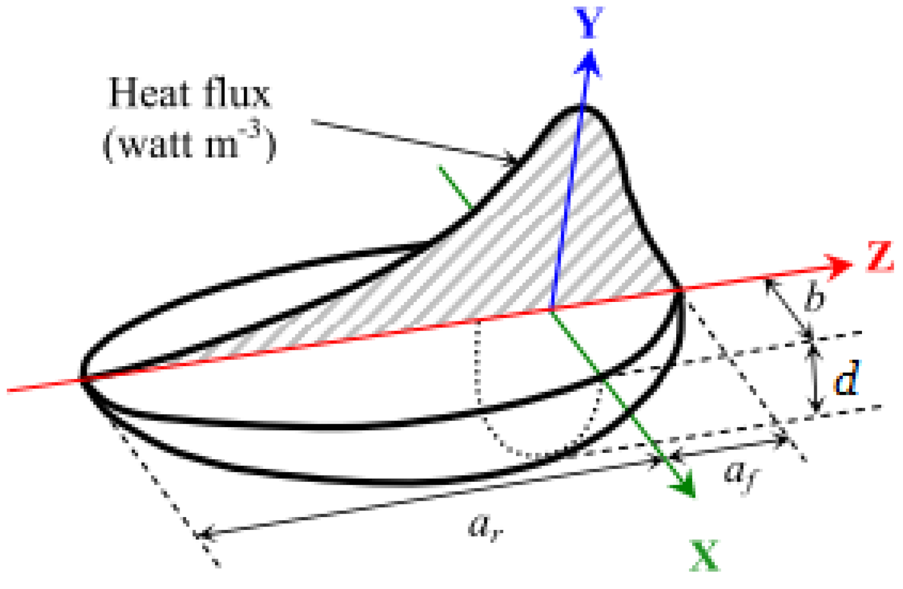
| af (m) | ar (m) | b (m) | d (m) | af (m) | ar (m) | b (m) | d (m) |
| 0.00245 | 0.0098 | 0.00245 | 0.00403 | 0.0043 | 0.0172 | 0.0043 | 0.00376 |

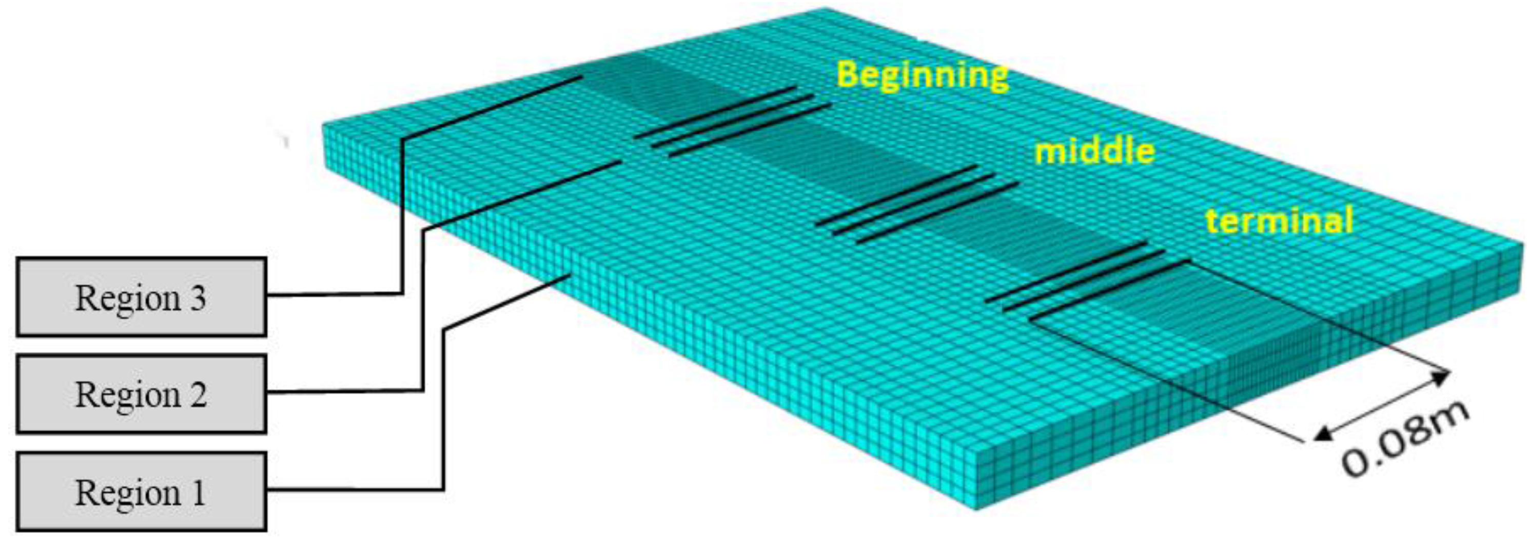
| Model | Number of Elements | |||
|---|---|---|---|---|
| Region 1 | Region 2 | Region 3 | Total | |
| Thermal | 24,480 | 41,616 | - | 66,096 |
| Thermo-mechanical | 3640 | 4480 | 5600 | 13,720 |

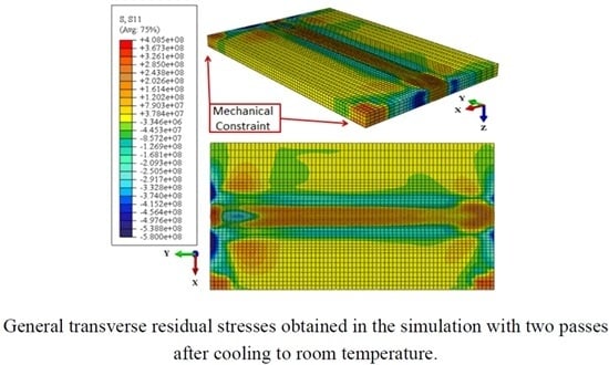
4. Results and Discussion

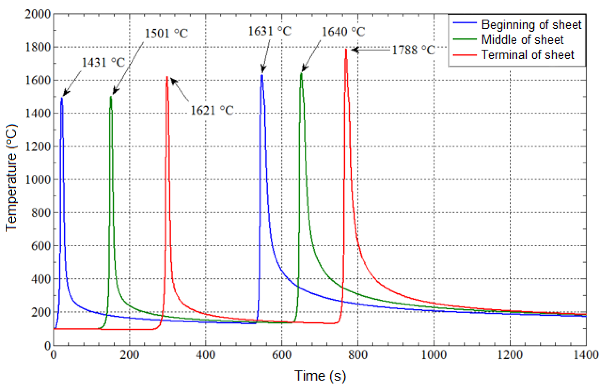
| ∆t8/5 Beginning (s) | ∆t8/5 Middle (s) | ∆t8/5 Terminal (s) | ∆t8/5 Average (s) | Variation (%) | |
|---|---|---|---|---|---|
| 1° pass | 3.71 | 4.02 | 3.30 | 3.68 | 22.00 |
| 2° pass | 22.50 | 26.89 | 27.30 | 25.56 | 21.00 |

5. Conclusions
Acknowledgments
Author Contributions
Conflicts of Interest
References
- Soul, F.; Hamdy, N. Numerical Simulation of Residual Stress and Strain Behavior after Temperature Modification. In Welding Processes; Kovacevic, R., Ed.; InTech: Rijeka, Croatia, 2012; Chapter 10. [Google Scholar] [CrossRef]
- Araújo, B.A.; Maciel, T.M.; Carrasco, J.P.; Vilar, E.O.; Silva, A.A. Evaluation of the diffusivity and susceptibility to hydrogen embrittlement of API 5L X80 steel welded joints. Intl. J. Multiphys. 2013. [Google Scholar] [CrossRef]
- Carlone, P.; Citarella, R.; Lepore, M.; Palazzo, G.S. A FEM-DBEM investigation of the influence of process parameters on crack growth in aluminum friction stir welded butt joints. Int. J. Mater. Form. 2015, 8, 591–599. [Google Scholar] [CrossRef]
- Citarella, R.; Carlone, P.; Lepore, M.; Palazzo, G.S. Numerical-experimental crack growth analysis in AA2024-T3 FSWed butt joints. Adv. Eng. Softw. 2015, 80, 47–57. [Google Scholar] [CrossRef]
- Jiang, W.; Fan, Q.; Gong, J. Optimization of welding joint between tower and bottom flange based on residual stress considerations in a wind turbine. Energy 2010, 35, 461–467. [Google Scholar] [CrossRef]
- Forouzan, M.R.; Heidari, A.; Golestaneh, S.J.F. FE simulation of submerged arc welding of API 5L-X70 straight seam oil and gas pipes. J. Comput. Methods Eng. 2009, 28, 93–110. [Google Scholar]
- Cho, J.R.; Lee, B.Y.; Moon, Y.H.; van Tyne, C.J. Investigation of residual stress and post weld heat treatment of multi-pass welds by finite element method and experiments. J. Mater. Proc. Technol. 2004, 155–159, 1690–1695. [Google Scholar] [CrossRef]
- Robertsson, A.; Svedman, J. Welding Simulation of a Gear Wheel Using FEM; Chalmers University of Technology (Department of Applied Mechanics): Göteborg, Sweden, 2013. [Google Scholar]
- Akbari, D.; Sattari-Far, I. Effect of the welding heat input on residual stresses in butt-welds of dissimilar pipe joints. Int. J. Press. Vessels Pip. 2009, 86, 769–776. [Google Scholar] [CrossRef]
- Syahroni, N.; Hidayat, M.I.P. 3D Finite Element Simulation of T-Joint Fillet Weld: Effect of Various Welding Sequences on the Residual Stresses and Distortions. In Numerical Simulation—From Theory to Industry; Andriychuk, M., Ed.; InTech: Rijeka, Croatia, 2012; Chapter 24. [Google Scholar] [CrossRef]
- Nóbrega, J.A.; Diniz, D.D.S.; Melo, R.H.F.; Araújo, B.A.; Maciel, T.M.; Silva, A.A.; Santos, N.C. Numerical evaluation of multipass welding temperature field in API 5L X80 steel welded joints. Int. J. Multiphys. 2014. [Google Scholar] [CrossRef]
- Goldak, J.; Chakravarti, A. A new finite element model for welding heat sources. Metall. Trans. 1984, 15, 299–305. [Google Scholar] [CrossRef]
- Queresh, E.M. Analysis of Residual Stresses and Distortions in Circumferentially Welded Thin-Walled Cylinders. Ph.D. Thesis, National University of sciences and Technology, Karachi, Pakistan, December 2008. [Google Scholar]
- Attarha, M.J.; Sattari-Far, I. Study on welding temperature distribution in thin welded plates through experimental measurements and finite element simulation. J. Mater. Proc. Technol. 2011, 211, 688–694. [Google Scholar] [CrossRef]
- Cooper, R.; Silva, J.H.F.; Trevisan, R.E. Influence of preheating on API 5L-X80-pipeline joint welding with self-shielded flux-cored wire. Weld. Int. 2005, 19, 882–887. [Google Scholar] [CrossRef]
- Araújo, B.A. Avaliação do Nível de Tensão Residual e Susceptibilidade à Fragilização Por Hidrogênio em Juntas Soldadas do Aço API 5L X80 Utilizados Para o Setor de Petróleo e Gás. Ph.D. Thesis, Universidade Federal de Campina Grande, Campina Grande, Brazil, September 2013. [Google Scholar]
- PETROBRAS. N-133 M: Welding (in Portuguese). Available online: http://sites.petrobras.com.br/CanalFornecedor/portugues/requisitocontratacao/requisito_normastecnicas.asp (accessed on 25 January 2016).
- Guimarães, P.B.; Pedrosa, P.M.A.; Yadava, Y.P.; Barbosa, J.M.A.; Filho, A.V.S.; Ferreira, R.A.S. Determination of residual stresses numerically obtained in ASTM AH36 steel welded by TIG process. Mater. Sci. Appl. 2013, 4, 268–274. [Google Scholar] [CrossRef]
- Depradeux, L. Simulation Numérique du Soudage—Acier 316L 2004. Validation Sur Cas Tests de Complexité Croissante. Ph.D. Thesis, INSA Lion, Lyon-Villeurbanne, France, 2004. [Google Scholar]
- Yao, X.; Zhu, L.-H.; Lim, V. Finite element analysis of residual stress and distortion in an eccentric ring induced by quenching. Trans. Mater. Heat Treat. 2004, 25, 746–751. [Google Scholar]
- Veiga, J.L.B.C. Analysis of Acceptance Criteria of Wrinkles in Pipeline Cold Bends. M.Sc. Thesis, Pontifícia Universidade Católica do Rio de Janeiro, Rio de Janeiro, Brazil, May 2009. [Google Scholar]
- Deng, D. FEM prediction of welding residual stress and distortion in carbon steel considering phase transformation effects. Mater. Des. 2009, 30, 359–366. [Google Scholar] [CrossRef]
- Stenbacka, N. On arc efficiency in Gas Tungsten Arc Welding. Soldagem e Inspeção 2013, 18, 380–390. [Google Scholar] [CrossRef]
- Abaqus/CAE User manual, version 6.3; Hibbit, Karlsson & Sorenson Inc.: Providence, RI, USA, 2007.
- Jiang, W.G. The development and applications of the helically symmetric boundary conditions in finite element analysis. Commun. Numer. Methods Eng. 1999, 15, 435–443. [Google Scholar] [CrossRef]
- Incropera, F.P.; DeWitt, D.P.; Bergman, T.L.; Lavine, A.S. Fundamentals of Heat and Mass Transfer, 7th ed.; John Wiley & Sons: Hoboken, NJ, USA, 2011. [Google Scholar]
- Laursen, A.; Maciel, T.M.; Melo, R.H.F. Influence of weld thermal cycle on residual stress of API 5L X65 and X70 welded joint. In Proceedings of the 2014 Canweld Conference, Vancouver, BC, Canada, 1 October 2014.
- Gery, D.; Long, H.; Maropoulos, P. Effects of welding speed, energy input and heat source distribution on temperature variations in butt joint welding. J. Mater. Proc. Technol. 2005, 167, 393–401. [Google Scholar] [CrossRef]
- Heinze, C.; Schwenk, C.; Rethmeier, M. Numerical calculation of residual stress development of multi-pass gas metal arc welding. J. Constr. Steel Res. 2012, 72, 12–19. [Google Scholar] [CrossRef]
- Kenneth, E. Fusion welding—Process variables. In Introduction to the Physical Metallurgy of Welding, 2nd ed.; Easterling, K., Ed.; Butterworth-Heinemann: Exeter, UK, 1992; Chapter 1; pp. 1–54. [Google Scholar] [CrossRef]
- Deng, D.; Kiyoshima, S. FEM prediction of welding residual stresses in a SUS304 girth-welded pipe with emphasis on stress distribution near weld start/end location. Comput. Mater. Sci. 2010, 50, 612–621. [Google Scholar] [CrossRef]
- Samardžić, I.; Čikić, A.; Dunđer, M. Accelerated weldability investigation of TStE 420 steel by weld thermal cycle simulation. Metalurgija 2013, 4, 461–464. [Google Scholar]
- Zhu, X.K.; Chao, Y.J. Effects of temperature-dependent material properties on welding simulation. Comput. Struct. 2012, 80, 967–976. [Google Scholar] [CrossRef]
- Nandan, R.; Roy, G.G.; Lienert, T.J.; DebRoy, T. Numerical modelling of 3D plastic flow and heat transfer during friction stir welding of stainless steel. Sci. Technol. Weld. Join. 2006, 11, 526–537. [Google Scholar] [CrossRef]
- Stamenković, D.; Vasović, I. Finite element analysis of residual stress in butt welding two similar plates. Sci. Tech. Rev. 2009, 59, 57–60. [Google Scholar]
© 2016 by the authors; licensee MDPI, Basel, Switzerland. This article is an open access article distributed under the terms and conditions of the Creative Commons by Attribution (CC-BY) license (http://creativecommons.org/licenses/by/4.0/).
Share and Cite
Da Nóbrega, J.A.; Diniz, D.D.S.; Silva, A.A.; Maciel, T.M.; De Albuquerque, V.H.C.; Tavares, J.M.R.S. Numerical Evaluation of Temperature Field and Residual Stresses in an API 5L X80 Steel Welded Joint Using the Finite Element Method. Metals 2016, 6, 28. https://doi.org/10.3390/met6020028
Da Nóbrega JA, Diniz DDS, Silva AA, Maciel TM, De Albuquerque VHC, Tavares JMRS. Numerical Evaluation of Temperature Field and Residual Stresses in an API 5L X80 Steel Welded Joint Using the Finite Element Method. Metals. 2016; 6(2):28. https://doi.org/10.3390/met6020028
Chicago/Turabian StyleDa Nóbrega, Jailson A., Diego D. S. Diniz, Antonio A. Silva, Theophilo M. Maciel, Victor Hugo C. De Albuquerque, and João Manuel R. S. Tavares. 2016. "Numerical Evaluation of Temperature Field and Residual Stresses in an API 5L X80 Steel Welded Joint Using the Finite Element Method" Metals 6, no. 2: 28. https://doi.org/10.3390/met6020028