Influence of Layer-Thickness Proportions and Their Strength and Elastic Properties on Stress Redistribution during Three-Point Bending of TiB/Ti-Based Two-Layer Ceramics Composites

Abstract

A mathematical model was developed to determine the order of failure of layers in a two-layer ceramics composite and to determine the conditions for achieving the maximum limit load under three-point loading. The model was set in the space of three “bilayer parameters”: the ratio of the thickness of the lower layer to the whole thickness of the beam, the ratio of Young’s moduli of the lower layer to the upper layer, and the ratio of flexural strengths of the materials of the lower layer to the upper layer. The adequacy of the model obtained was confirmed by experimental results on the three-point bending of the experimental specimens. The experimental samples were two-layer composites consisting of a cermet layer TiB/Ti and a layer of α-Ti. The samples were obtained by free self-propagating high-temperature synthesis (SHS) compression and with varying their thickness. The results obtained make it possible to predict in advance which layer, based on the specific bilayer parameters, will trigger the brittle fracture mechanism as well as to set the maximum destructive load of bilayer composites.

1. Introduction

To date, composite materials based on titanium borides are of great scientific and practical interest. These materials provide the highest specific strength and modulus of elasticity compared to steel and nickel alloys, while their density is significantly lower [1,2,3,4,5]. However, the requirements to the physical–mechanical and operational properties of composite materials are increasing every year due to their work in heavier and more loaded conditions. The main influences on the properties of composites are the methods of their production and the proportion and structure of borides in the volume of the material. Titanium composite materials with TiB₂- [6,7,8,9,10] and TiB [11,12,13,14,15,16,17,18]-strengthening phases have been extensively studied. The structure of titanium borides is strongly influenced by high degrees of material deformation, which lead to significant grain refinement and texture formation [18,19]. It can also be noted that composite materials based on titanium borides have lower strength properties with increasing temperature compared to monolithic materials due to the higher heat resistance of titanium monoboride fibers.

One promising direction to improve the properties is the development of a special design of layered composite material (LCM) consisting of alternating layers [20,21,22,23,24]. For LCM, a significant influence is exerted by the interlayer boundaries, which contribute to crack branching and their rebirth in each new layer. This leads to improved crack resistance and fatigue properties compared to monolithic materials [25,26,27]. In addition, the development of a new LCM design can provide a unique combination of mechanical and performance characteristics, which are also not characteristic of monolithic materials [28,29,30,31]. In [32], layered composite materials based on the Ti₂AlNb/Ti₆Al₄V alloy were obtained by hot pressing. The authors found that the fracture toughness, K_IC, of the obtained LCM is more than two times higher than that of the Ti₂AlNb monolithic alloy. The increase in the fracture toughness value is explained by the authors precisely by the layered structure of the composite, in which, under loading at the boundaries between the layers, the stress concentration decreases, and the connection of emerging cracks is also prevented. In [33], LCM was obtained by vacuum hot pressing based on TiBw/Ti₃Al-Ti₃Al, which also had fracture toughness increased by 15% compared to a monolithic material based on Ti₃Al.

When developing the LCM design, an important task is to establish the influence of layer-thickness proportions and their elastic properties on stress redistribution and, as a consequence, on ultimate loads. Our study required a significant narrowing of the available theories of flexural strength of layered composites. We began by assuming that each layer is homogeneous and isotropic and does not require averaging of its properties [34]. Due to the high strength of the diffusion character of the connection of the layers in the material in question, we did not consider the delamination conditions [35]. We did not consider any damage mechanics time-dependent effects in our case [36].

We took the criterion of maximum stress [37] as the criterion for fracture of the layer in a two-layer beam. Moreover, we introduced a simplification to the maximum stress criterion and considered reaching the limit value of the stress tensor component along the x-axis as the failure criterion. We estimated the value of this simplification further. And finally, we constructed first-ply failure criteria [38] for the three-point loading case for two-layered composite material. The approach to the analysis of the stress state of the beam within the Bernoulli–Euler model led to a good correlation with the experimental data. In case of more accurate analysis, it is possible to develop this methodology to the Timoshenko or Reddy–Levinson beam model [39].

To this end, mathematical modeling of the failure process of LCM based on two-layer material TiB/Ti under three-point bending was performed in the present work. The novelty of this study is that we are able to predict in advance which layer, based on the specific parameters of the two-layer material, will trigger the brittle fracture mechanism. We can determine the effect of the flexural strength of each layer on the order of their failure and ultimately on the combined strength of the two-layer composite. To estimate the adequacy of the developed model, experiments on three-point bending of specimens obtained by free SHS compression were performed [40,41].

The fracture of the specimens in the experiment fixes the ultimate load, which is an integral factor of influence of the layers flexural strengths, the distribution of defects in them, and the proportions of their elastic properties and thicknesses. The work investigates the contribution of each parameter mentioned, called bilayer parameters. Bending strength in TiB/Ti material [42] is correlated with our parameter, considered as TiB/Ti layer flexural strength. Moreover, for the wide range of both layers’ strength value, the maximum value of flexural strength is 1989.35 MPa [43]. We are able to obtain the map critical load level for the three-point loading test in the space of three two-layer parameters, which are considered here. Previously, similar dependences have not been obtained by other researchers for cermet multilayer composites.

2. Objects and Methods of Research

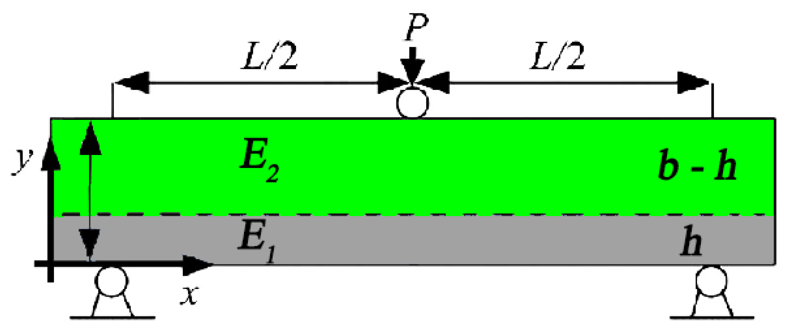
2.1. Statement of the Problem

To carry out mathematical modeling, we considered a beam of rectangular cross-section $S$ from the layers of two different thicknesses of elastic homogeneous materials under conditions of three-point loading. Let us denote that the lower layer opposite to the side of the load application $P$ by the index 1 and the upper layer by the index 2. The thickness of the layers and their proportions may vary, but the sum of the thicknesses is equal to a fixed value of the beam thickness $b$.

Let us point the x-axis horizontally along the axis of the beam and the y-axis orthogonal to the x-axis, upwards in thickness. The z axis is orthogonal to the xy plane along the beam width $a$ (Figure 1), L is the distance between supports under three-point loading, $h$ is the thickness of the bottom layer, and $b-h$ is the thickness of the top layer (Figure 1).

For the chosen coordinate system, we considered the normal components of elastic stresses $\sigma \left(x,y\right)$ along the section at the point $x$, orthogonal to the neutral axis whose coordinate is $y_0(x)$. $E\left(y\right)$ is Young’s modulus; $\kappa (x)$ is the curvature of the neutral axis. The change of stresses along the coordinate z is negligible. We also assumed that the ratio between the supports distance and the beam thickness is large enough to disregard the influence of the tangential components of the stress.

Let us introduce three bilayer parameters: $\hspace{0.33em}\gamma =E_1/E_2$ is the ratio of the Young’s modulus of the lower layer to the upper layer, $\eta =h/b$ is the ratio of the thickness of the lower layer to the whole thickness of the beam, and $\lambda ={\sigma }_{*1}/{\sigma }_{*2}$ is the ratio of the flexural strength of the lower layer to the upper layer.

The following is required:

• To determine the region of bilayer parameters in which brittle failure will begin in the upper layer earlier than in the lower layer;
• To determine the strength of the beam materials based on the ultimate load and bilayer parameters.

Below are the parameters used and their designations and definitions:

Variable, Parameter	Definition
$a$	, beam width;
$b$	, beam thickness;
$S$	, beam cross-section;
$h$	, bottom-layer thickness;
$b-h$	, top-layer thickness;
$L$	, supports distance;
x, y, z	, Cartesian coordinates;
$y_0(x)$	, neutral axis coordinate;
$\kappa (x)$	, neutral axis curvature
P	Load;
$E\left(y\right)$	, Young’s modulus;
$E_1$	, bottom-layer Young’s modulus;
$E_2$	, top-layer Young’s modulus;
$\hspace{0.33em}\gamma =E_1/E_2$	, bilayer parameter for Young’s modulus ratio;
$\eta =h/b$	, bilayer parameter for bottom-layer-thickness ratio;
$\lambda ={\sigma }_{*1}/{\sigma }_{*2}$	, bilayer parameter for layers’ flexural strength ratio;
$\sigma \left(x,y\right)$	, normal component of the stress tensor in the beam cross-section;
$\Delta$	, diffusion interlayer zone thickness;
$\chi =x/L$	, dimensionless coordinate along beam axis;
$\psi =y/b$	, dimensionless coordinate orthogonal beam axis along y;
$\zeta =z/b$	, dimensionless coordinate orthogonal beam axis along z;
$\xi =y_0/b$	, dimensionless neutral axis coordinate;
$\delta =\Delta /b$	, dimensionless diffusion interlayer zone thickness;
$l=L/b$	, dimensionless supports distance;
$p=\frac{1}{2E_2}\frac{P}{S}$	, dimensionless load;
${\sigma }_{\chi \chi }$, ${\sigma }_{\psi \psi }$, ${\sigma }_{\chi \psi }$, ${\sigma }_{\chi \psi }$	, component of the stress tensor in $\chi ,\psi ,\zeta$ coordinates;
$k=\kappa \left(1/2\right)$	, neutral axis curvature in the beam center;
$\alpha$	, maximum stress deflection angle of the x-axis;
${\epsilon }_e$	, elastic limit for bottom-layer material;
${\chi }_e$, ${\psi }_e$	, elastic zone dimensionless x,y coordinates for bottom layer;
$E_t$	, tangential modulus;
${\gamma }_t=E_t/E_1$	, tangential and Young’s modulus ratio for bottom layer.

2.2. Subjects of Research

Two-layer samples consisting of a cermet layer TiB-40 wt.%Ti (TiB/Ti) and an alpha-titanium (α-Ti) layer, which were obtained by free SHS compression, were chosen as an experimental object of research. This method makes it possible to obtain composite materials from the initial powder components (titanium and boron) in tens of seconds by combining the processes of combustion in the mode of self-propagating high-temperature synthesis [44,45] and shear high-temperature deformation [30,31]. In this method, the phase- and structure-formation processes proceed under extreme conditions in fractions of a second and at high temperatures (over 2000 °C), which introduces significant changes into the structure and properties of the obtained materials. The scheme of the process of obtaining two-layer composites is shown in Figure 2.

As the starting powders, we took commercial powders of 89 wt.% titanium (<45 µm, 99.1%) and 11 wt.% boron (<1 µm, 99.7%), from which a green sample with the dimensions 45 × 80 × 22 mm with the relative density of 0.75 was pressed. The green sample was placed on a 1–1.5 mm thick alpha-titanium substrate. The chemical reaction between boron and titanium was initiated by a tungsten spiral, to which an alternating voltage of 30 V was applied. After the combustion wave passed from the helix to the opposite edge of the green sample and the specified delay time, the synthesized material was pressed at a pressure of 30 MPa. Due to the absence of side walls, the synthesized material was subjected to shear deformation in addition to volumetric compaction (in Figure 2, the direction of shear is shown by red arrows).

The number of pores and defects in the synthesized material decreased due to shear deformation. Due to the high combustion temperature of the studied composition (2100 °C), the titanium substrate surface melted, and the diffusion zone between the cermet material and the titanium substrate was formed under the action of external pressure. The delay time before pressure application and the value of the applied pressure allowed to regulate the size of the diffusion zone and the structure of the resulting composite. By varying the initial dimensions of the green sample and the titanium substrate, it was possible to obtain composites with specified dimensions and physical and mechanical properties. In this work, two-layer cermet composites with dimensions 55 × 90 × 10 mm were obtained by free SHS compression, from which samples of rectangular cross-section with dimensions 7.1 × 3.95 × 50 mm were cut out by electro-erosion cutting. The considered type of cermet materials on the basis of TiB/Ti is characterized by brittle character of fracture, high hardness, and rigidity of the material in general and the adhesion layer in particular. The cermet layer is located on a plastic matrix of alpha-titanium. The papers [46,47,48,49,50] describe the structure of these materials and their physical and mechanical properties.

Table 1. Properties of experimental samples and experimental results.

Sample Number	Distance between Supports, L mm	Sample Width, a mm	Sample Thickness, b mm	Bottom-Layer Thickness h mm	$\mathsf{\eta }=\mathit{h}/\mathit{b}$	Max. Force, P* N	Bending Strength Limit of the Top Layer TiB, ${\mathsf{\sigma }}_2^{*}$ MPa	Bending Strength Limit of the Bottom Layer TiB, ${\mathsf{\sigma }}_1^{*}$ MPa	${\mathit{E}}_2$ GPa	${\mathit{E}}_1$ GPa
S1	42.7	3.95	7.1	1	0.140	1486.2	564	1100	407	110
S2				1.1	0.155	1534.8
S3				1.2	0.169	1782.4
S4				3.5	0.493	2614.5
S5				3.6	0.507	2651.8
S6				0.98	0.138	1548.6
S7				0.92	0.130	1821.8
S8				0.85	0.120	1525.8

shows the properties of experimental samples and experimental results.

2.3. Research Methods

Experiments on three-point bending were carried out on the universal compression machine REM-20 according to GOST 28840 and STO-75829762-001. The microstructure was studied using a Carl Zeiss Ultraplus ultra-high resolution auto-emission scanning electron microscope (Carl Zeiss, Neubeuern, Germany) as well as an Altami Met 1 C metallographic microscope (Altami, Saint-Petersburg, Russia).

3. Results and Discussion

3.1. Model Development

3.1.1. The Elastic Case: Finding Stresses

Because of the special rigidity of the obtained SHS materials, it is appropriate to solve the problem in the framework of the Bernoulli–Euler beam model [39]. Let us also assume that in the diffusion layer, the elastic properties change linearly from material 1 to material 2:

$$\begin{array}{l}\sigma \left(x,y\right)=\kappa (x)E\left(y\right)\left(y_0-y\right),\hspace{0.33em}\\ E\left(y\right)=\left\{\begin{array}{l}{E}_2,\hspace{1em}y\in (h+1/2\Delta ,b]\\ \frac{\left(E_2+E_1\right)}{2}+\left(E_2-E_1\right)\frac{\left(y-h\right)}{\Delta },\hspace{0.33em}y\in [h-1/2\Delta ,h+1/2\Delta ]\\ E_1,\hspace{1em}y\in [0,h-1/2\Delta )\end{array}\right.\end{array}$$

(1)

Let us introduce dimensionless coordinates and parameters:

$$\chi =\frac{x}{L},\hspace{0.33em}\psi =\frac{y}{b},\hspace{0.33em}\xi =\frac{y_0}{b},\hspace{0.33em}\delta =\frac{\Delta }{b},\hspace{0.33em}\hspace{0.33em}l=\frac{L}{b},\hspace{0.33em}p=\frac{1}{2E_2}\frac{P}{S}$$

(2)

Let us write a system of equilibrium equations for longitudinal forces and moments here and below for the longitudinal dimensionless coordinate $\chi \in [0,1/2]$; the other half of the beam is symmetrical.

$$\begin{array}{l}{\displaystyle \underset{0}{\overset{\eta -1/2\delta }{\int }}\gamma \left(\xi -\psi \right)d\psi }+{\displaystyle \underset{\eta -1/2\delta }{\overset{\eta +1/2\delta }{\int }}\frac{2\left(1-\gamma \right)\left(\psi -\eta \right)+\left(1+\gamma \right)\delta }{2\delta }\left(\xi -\psi \right)d\psi }+{\displaystyle \underset{\eta +1/2\delta }{\overset{1}{\int }}\left(\xi -\psi \right)d\psi }=0\\ {\displaystyle \underset{0}{\overset{\eta -1/2\delta }{\int }}\gamma {\left(\xi -\psi \right)}^{2}d\psi }+{\displaystyle \underset{\eta -1/2\delta }{\overset{\eta +1/2\delta }{\int }}\frac{2\left(1-\gamma \right)\left(\psi -\eta \right)+\left(1+\gamma \right)\delta }{2\delta }{\left(\xi -\psi \right)}^{2}d\psi }+{\displaystyle \underset{\eta +1/2\delta }{\overset{1}{\int }}{\left(\xi -\psi \right)}^{2}d\psi }=\frac{pl\chi }{\kappa \left(\chi \right)}\end{array}$$

(3)

From the equation of force equilibrium, we obtain the coordinate of the neutral axis.

$$\xi =\frac{1}{2}\frac{1-{\eta }^2\left(1-\gamma \right)}{1-\eta \left(1-\gamma \right)}-\frac{1}{24}{\delta }^2\frac{\left(1-\gamma \right)}{1-\eta \left(1-\gamma \right)}$$

(4)

Let us consider how the neutral axis is located relative to the separation zone. This will affect the form of equilibrium equations. The case when the neutral axis coincides at the initial moment of time with the diffusion layer corresponds to the following condition:

$$\eta =\frac{1}{1+\sqrt{\gamma }}$$

(5)

Under the condition $0<\eta <1/\left(1+\sqrt{\gamma }\right)$, the neutral axis will be above the layer interface. Under the condition $1/\left(1+\sqrt{\gamma }\right)<\eta <1$, the neutral axis will be below the layer interface.

We express the curvature of the neutral axis from the momentum equilibrium equation:

$$\kappa \left(\chi \right)=12pl\chi {\left[\frac{\left(\left(\gamma -1\right)\left(\gamma {\eta }^4-{\left(\eta -1\right)}^4\right)+\gamma \right)}{\left(1+\eta \left(\gamma -1\right)\right)}+\frac{3{\delta }^2}{2}\frac{\left(\gamma -1\right)\left(\gamma {\eta }^2-{\left(\eta -1\right)}^2\right)}{\left(1+\eta \left(\gamma -1\right)\right)}-\frac{5{\delta }^4}{48}\frac{{\left(\gamma -1\right)}^2}{\left(1+\eta \left(\gamma -1\right)\right)}\right]}^{-1}$$

(6)

Substituting Equation (6) in Equation (1), we obtain the following:

$$\sigma \left(\chi ,\psi \right)=\left\{\begin{array}{l}{E}_2\kappa (\chi )\left(\xi -\psi \right),\hspace{1em}\psi \in (\eta +1/2\delta ,1]\\ E_2\kappa \left(\chi \right)\left[\frac{\left(1+\gamma \right)}{2}+\left(\gamma -1\right)\frac{\left(\psi -\eta \right)}{\delta }\right]\left(\xi -\psi \right),\psi \in [\eta -1/2\delta ,\eta +1/2\delta ]\\ E_2\gamma \kappa (\chi )\left(\xi -\psi \right),\hspace{1em}\psi \in [0,\eta -1/2\delta )\end{array}\right.$$

(7)

Due to the stress linear dependence, the maximum will be reached at the lower edge of the layer. At an essentially small thickness of the diffusion layer $\left(\delta \ll {10}^{-6}\right)$, in further calculations, we will neglect it and use the following equations:

$$\xi =\frac{1}{2}\frac{1-{\eta }^2\left(1-\gamma \right)}{1-\eta \left(1-\gamma \right)},\hspace{1em}\kappa \left(\chi \right)=12\frac{\left(1-\eta \left(1-\gamma \right)\right)}{\left(\left(1-\gamma \right)\left({\left(1-\eta \right)}^4-\gamma {\eta }^4\right)+\gamma \right)}pl\chi$$

(8)

And the stresses will be in the following form:

$$\sigma \left(\chi ,\psi \right)=\left\{\begin{array}{l}{E}_2\kappa (\chi )\left(\xi -\psi \right),\hspace{1em}\psi \in (\eta ,1]\\ E_2\gamma \kappa (\chi )\left(\xi -\psi \right),\hspace{1em}\psi \in [0,\eta ]\end{array}\right.$$

(9)

In this case, the maximum stress ${\sigma }_m$ in the central section of the beam on the opposite edge of the beam to the point of force application will be in the upper layer:

$${\sigma }_{m2}=\frac{3}{2}l\frac{{\left(1-\eta \right)}^2-\gamma {\eta }^2}{\gamma +\left(\gamma -1\right)\left(\gamma {\eta }^4-{\left(\eta -1\right)}^4\right)}\frac{P}{S}$$

(10)

Maximum stress in the lower layer is as follows:

$${\sigma }_{m1}=\frac{3}{2}l\gamma \frac{1+{\eta }^2\left(\gamma -1\right)}{\gamma +\left(\gamma -1\right)\left(\gamma {\eta }^4-{\left(\eta -1\right)}^4\right)}\frac{P}{S}$$

(11)

Then, the ratio of maximum stresses in the central cross-section of the beam will be as given:

$$\frac{{\sigma }_{m1}\left(\psi =0\right)}{{\sigma }_{m2}\left(\psi =\eta \right)}=\gamma \frac{\xi }{\left(\xi -\eta \right)}=\gamma \frac{1+{\eta }^2\left(\gamma -1\right)}{{\left(1-\eta \right)}^2-{\eta }^2\gamma }$$

(12)

The condition of the beginning of fracture in the upper layer 2 before the lower layer 1, taking into account that the neutral axis must be above the zone of layer separation, gives a system of inequalities for the bilayer parameters:

$$\lambda >\gamma \frac{1-{\eta }^2\left(1-\gamma \right)}{{\left(1-\eta \right)}^2-{\eta }^2\gamma },\hspace{1em}0<\eta <\frac{1}{1+\sqrt{\gamma }}$$

(13)

The system of inequalities (12) can be visualized with a fixed parameter of the ratio of the Young’s modulus of the lower layer to the upper layer $\gamma$. The parameter of the strength ratio of the layers $\lambda$ will lie above each graph in Figure 3.

Curves on the Figure 3 demonstrates shape of equation $\lambda =\gamma \frac{1-{\eta }^2\left(1-\gamma \right)}{{\left(1-\eta \right)}^2-{\eta }^2\gamma }$ for the different proportions of Young’s moduli $\gamma =0.1,\hspace{0.33em}0.2,\hspace{0.33em}0.5,\hspace{0.33em}1,\hspace{0.33em}2,\hspace{0.33em}5$ and delimits the area’s initial failure of the upper or lower layer for different volumes of flexural strength ratio parameter $\lambda$. Figure 3 is a fracture map for the two-layered composite under three-point loading conditions.

3.1.2. Fracture Criterion of the Layer

Let us find the value of the maximum stress similarly to Timoshenko’s solution of the problem of considering tangential stresses in an elastic beam in three-point bending, assuming that transverse stresses have negligible influence: ${\sigma }_{yy}={\sigma }_{yz}={\sigma }_{zz}=0$. Solve the problem by the semi-inverse Saint–Venant method. Then, the system of equations will be in the following form:

$$\begin{array}{l}\left\{\begin{array}{l}\frac{\partial {\sigma }_{\chi \psi }}{\partial \psi }+\frac{\partial {\sigma }_{\chi \zeta }}{\partial z}=-\frac{1}{l}\frac{\partial {\sigma }_{\chi \chi }}{\partial \chi }\\ \frac{\partial {\sigma }_{\chi \psi }}{\partial \chi }=0\\ \frac{\partial {\sigma }_{\chi \zeta }}{\partial \chi }=0\end{array}\right.\hspace{1em}{\sigma }_{\chi \psi }\left(\chi ,0\right)={\sigma }_{\chi \psi }\left(\chi ,1\right)=0\hspace{1em}\\ {\sigma }_{\chi \chi }\left(\chi ,\psi \right)=\left\{\begin{array}{l}{E}_2\kappa (\chi )\left(\xi -\psi \right),\hspace{1em}\psi \in (\eta +1/2\delta ,1]\\ E_2\kappa \left(\chi \right)\left[\frac{\left(1+\gamma \right)}{2}+\left(\gamma -1\right)\frac{\left(\psi -\eta \right)}{\delta }\right]\left(\xi -\psi \right),\psi \in [\eta -1/2\delta ,\eta +1/2\delta ]\\ E_2\gamma \kappa (\chi )\left(\xi -\psi \right),\hspace{1em}\psi \in [0,\eta -1/2\delta )\end{array}\right.\end{array}$$

(14)

As a result of solution, we obtain the following in the center cross-section, where $k=\kappa \left(1/2\right)$:

$${\sigma }_{\chi \psi }=\left\{\begin{array}{l}\frac{k}{2}\frac{b}{L}\left(\psi -1\right)\left(\psi -2\xi +1\right),\hspace{1em}\psi \in (\eta +1/2\delta ,1]\\ -k\frac{b}{L}\left[\begin{array}{l}-\frac{1}{3}\frac{\left(\gamma -1\right)}{\delta }{\psi }^3+\left(\frac{1}{2}+\frac{1}{2}\gamma -\frac{\left(\gamma -1\right)\eta }{\delta }\right)\xi \psi +\\ +\frac{1}{2}\left(-\frac{1}{2}-\frac{1}{2}\gamma +\frac{\left(\gamma -1\right)\eta }{\delta }+\frac{\left(\gamma -1\right)\xi }{\delta }\right){\psi }^2+C_0\end{array}\right],\psi \in [\eta -1/2\delta ,\eta +1/2\delta ],\\ -\gamma \frac{k}{2}\frac{b}{L}\left(2\xi \psi -{\psi }^2\right),\hspace{1em}\psi \in [0,\eta -1/2\delta )\end{array}\right.$$

(15)

Note that at the dependence point $\psi =\eta$, the functions describing tangential stresses in the upper and lower layers differ by the value $\frac{1}{24}{\delta }^{2}k\left(\gamma -1\right)$, independent of the proportion of layers and by an order of magnitude smaller than the square of the parameter of the share of the diffusion layer in the total thickness of the beam. Formally, we can define the constant $C_0$ as half of this difference.

Further, we will neglect this layer and set the distribution of tangential stresses ${\sigma }_{\chi \psi }$ and axial stresses ${\sigma }_{\chi \chi }$ in the form of piecewise smooth functions:

$$\begin{array}{l}{\sigma }_{\chi \psi }=\left\{\begin{array}{l}k/\left(2l\right)\left(\psi -1\right)\left(\psi -2\xi +1\right),\hspace{1em}\psi \in [\eta ,1]\\ \gamma k/\left(2l\right)\psi \left(\psi -2\xi \right),\hspace{1em}\psi \in [0,\eta )\end{array}\right.\\ {\sigma }_{\chi \chi }=\left\{\begin{array}{l}k\left(\xi -\psi \right)\chi ,\hspace{1em}\psi \in [\eta ,1]\\ \gamma k\left(\xi -\psi \right)\chi ,\hspace{1em}\psi \in [0,\eta )\end{array}\right.\end{array}$$

(16)

The tangent of the angle of the area with maximum normal stress is as follows:

$$tg\left(2\alpha \right)=-2\frac{{\sigma }_{\chi \psi }}{{\sigma }_{\chi \chi }}=\left\{\begin{array}{l}-\frac{\psi \left(\psi -2\xi \right)}{l\left(\xi -\psi \right)\chi }+\frac{\left(1-2\xi \right)}{l\left(\xi -\psi \right)\chi },\hspace{1em}\psi \in [\eta ,1]\\ -\frac{\psi \left(\psi -2\xi \right)}{l\left(\xi -\psi \right)\chi },\hspace{1em}\psi \in [0,\eta )\end{array}\right.$$

(17)

Substitute an expression for the neutral axis coordinates, and we obtain the dependence of the tilt angle on the transverse coordinate:

$$\alpha =\left\{\begin{array}{l}\frac{1}{2}\arctan \left(-\frac{\psi \left(\psi -2\xi \right)}{l\left(\xi -\psi \right)\chi }+\frac{\left(1-2\xi \right)}{l\left(\xi -\psi \right)\chi }\right),\hspace{1em}\psi \in [\eta ,1]\\ \frac{1}{2}\arctan \left(-\frac{\psi \left(\psi -2\xi \right)}{l\left(\xi -\psi \right)\chi }\right),\hspace{1em}\psi \in [0,\eta )\end{array}\right.$$

(18)

Let us define a value of maximal tensile force on this area:

$${\sigma }_{\max }={\sigma }_{\chi \chi }{\cos }^2\alpha +{\sigma }_{\chi \psi }\sin 2\alpha$$

(19)

Let us illustrate the given dependence of the value of maximum tensile stress on transverse coordinate $\psi$ at $\gamma =0.25$ and $\eta =0.25$ in $\chi =0.5$. The vertical line shows the interface between the two layers. Thus, taking into account that the maximum tensile stress gives a correction of the fracture stress at the edge of the upper layer 2 of not more than 0.1% and has no effect on the stress at the edge of the lower layer 1, we consider the following Figure 4.

3.1.3. Consideration of Elastic–Plastic Properties of the Lower Layer

Now, consider the case where the lower-layer material has a variable modulus of elasticity corresponding to an elastic–plastic strengthening material ($E_t$—tangential modulus) under active loading.

Until the linear elasticity limit is reached, the solution remains the same, that is, when the strains at all points of the lower layer are less than the limit strain ${\epsilon }_e$.

With increasing curvature at $\kappa >{\epsilon }_e/\xi$ will appear the boundary of separation of the lower layer into an elastic part and a hardening plastic part in active loading:

$${\psi }_e=\xi -{\epsilon }_e/\kappa \left(\chi \right)$$

(20)

And we will have to add the secant modulus of elasticity for the part of the lower layer:

$$\sigma \left(\chi ,\psi \right)=E\left(\psi \right)\kappa (\chi )\left(\xi -\psi \right),\hspace{0.33em}\hspace{1em}E\left(\psi \right)=\left\{\begin{array}{l}{E}_2,\hspace{1em}\psi \in (\eta ,1]\\ E_1,\hspace{1em}\psi \in ({\psi }_e,\eta ]\\ E_t+\left(E_1-E_t\right){\epsilon }_e/\left(\kappa \left(\chi \right)\left(\xi -\psi \right)\right),\hspace{1em}\psi \in [0,{\psi }_e]\end{array}\right.$$

(21)

As the load builds up, the entire bottom layer will be in plasticity, as provided:

$$\kappa \left(\chi \right)>{\epsilon }_e/\left(\xi -\eta \right),\hspace{1em}\xi >\eta$$

(22)

This is true for the neighborhood around the central section $\chi \in [1/2-{\chi }_e,1/2+{\chi }_e],\hspace{1em}\kappa \left({\chi }_e\right)={\epsilon }_e/\left(\xi -\eta \right)$. In this vicinity, the stresses will have the given form:

$$\sigma \left(\chi ,\psi \right)=E\left(\psi \right)\kappa (\chi )\left(\xi -\psi \right),\hspace{0.33em}\hspace{1em}E\left(\psi \right)=\left\{\begin{array}{l}{E}_2,\hspace{1em}\psi \in (\eta ,1]\\ E_2\gamma \left({\gamma }_t+\left(1-{\gamma }_t\right){\epsilon }_e/\left(\kappa \left(\chi \right)\left(\xi -\psi \right)\right)\right),\hspace{1em}\psi \in [0,\eta ]\end{array}\right.$$

(23)

Let us introduce another parameter, ${\gamma }_t=E_t/E_1<1$, and write the system of equilibrium equations of longitudinal forces and moments taking into account the hardening zone in dimensionless variables:

$$\begin{array}{l}{\displaystyle \underset{0}{\overset{\eta }{\int }}\left[{\gamma }_t+\left(1-{\gamma }_t\right){\epsilon }_e/\left(\kappa \left(\chi \right)\left(\xi -\psi \right)\right)\right]\gamma \left(\xi -\psi \right)d\psi }+{\displaystyle \underset{\eta }{\overset{1}{\int }}\left(\xi -\psi \right)d\psi }=0\\ {\displaystyle \underset{0}{\overset{\eta }{\int }}\left[{\gamma }_t+\left(1-{\gamma }_t\right){\epsilon }_e/\left(\kappa \left(\chi \right)\left(\xi -\psi \right)\right)\right]\gamma {\left(\xi -\psi \right)}^{2}d\psi }+{\displaystyle \underset{\eta }{\overset{1}{\int }}{\left(\xi -\psi \right)}^{2}d\psi }=\frac{pl\chi }{\kappa \left(\chi \right)}\hspace{1em}\end{array}$$

(24)

From the equation of force equilibrium, we obtain the coordinate of the neutral axis, which depends on the given curvature:

$$\xi =\frac{1}{2}\frac{1-{\eta }^2\left(1-\gamma {\gamma }_t\right)}{1-\eta \left(1-\gamma {\gamma }_t\right)}-\frac{\eta \gamma \left(1-{\gamma }_t\right)}{1-\eta \left(1-\gamma {\gamma }_t\right)}\frac{{\epsilon }_e}{\kappa \left(\chi \right)}$$

(25)

Consider how the neutral axis is located relative to the separation zone. This will affect the form of equilibrium equations. Considering the case when the neutral axis coincides at the initial moment of time with the diffusion layer as a boundary one, taking into account the positivity and unit limit of $\eta$, we obtain a condition on the thickness of layers relative to the elastic moduli when the neutral axis is above the interface:

$$\eta <\frac{\left(1+\gamma \left(1-{\gamma }_t\right){\epsilon }_e/\kappa \left(\chi \right)\right)-\sqrt{2\gamma \left(1-{\gamma }_t\right){\epsilon }_e/\kappa \left(\chi \right)+{\gamma }^2{\left(1-{\gamma }_t\right)}^2{\epsilon }^2{}_e/{\kappa }^2\left(\chi \right)+\gamma {\gamma }_t}}{\left(1-\gamma {\gamma }_t\right)}$$

(26)

From the equation of moment equilibrium, we obtain the dependence for the curvature:

$$\kappa (\chi )=12\frac{\left(1-\eta \left(1-\gamma {\gamma }_t\right)\right)}{\left(1-\gamma {\gamma }_t\right)\left({\left(\eta -1\right)}^4-\gamma {\gamma }_t{\eta }^4\right)+\gamma {\gamma }_t}lp\chi -6\frac{\left(1-{\gamma }_t\right)\left(1-\eta \right)\gamma \eta {\epsilon }_e}{\left(1-\gamma {\gamma }_t\right)\left({\left(\eta -1\right)}^4-\gamma {\gamma }_t{\eta }^4\right)+\gamma {\gamma }_t}$$

(27)

And the position of the neutral axis will be determined:

$$\xi \left(\chi \right)=\frac{1}{2}\frac{1-{\eta }^2\left(1-\gamma {\gamma }_t\right)}{1-\eta \left(1-\gamma {\gamma }_t\right)}-\frac{{\epsilon }_e\eta \gamma \left(1-{\gamma }_t\right)\left(\left(1-\gamma {\gamma }_t\right)\left({\left(\eta -1\right)}^4-\gamma {\gamma }_t{\eta }^4\right)+\gamma {\gamma }_t\right)}{6\left(1-\eta \left(1-\gamma {\gamma }_t\right)\right)\left(2\left(1-\eta \left(1-\gamma {\gamma }_t\right)\right)lp\chi -{\epsilon }_e\gamma \eta \left(1-{\gamma }_t\right)\left(1-\eta \right)\right)}$$

(28)

In the elastic case, ${\gamma }_t=1$, and we obtain the neutral axis position and curvature as in Equation (8):

$${\xi }_e=\frac{1}{2}\frac{1-{\eta }^2\left(1-\gamma \right)}{1-\eta \left(1-\gamma \right)},\hspace{1em}{\kappa }_e\left(\chi \right)=12\frac{\left(1-\eta \left(1-\gamma \right)\right)}{\left(\gamma -\left(1-\gamma \right)\left({\left(1-\eta \right)}^4-\gamma {\eta }^4\right)\right)}pl\chi$$

(29)

Let us determine the stress values at the lower edges of both layers taking into account Equations (23), (27) and (28):

$$\begin{array}{l}{\sigma }_{m1}\left(\chi =\frac{1}{2},\psi =0\right)=E_1\left({\gamma }_t+\left(1-{\gamma }_t\right){\epsilon }_e/\left(\kappa \xi \right)\right)\kappa \xi \\ {\sigma }_{m2}\left(\chi =\frac{1}{2},\psi =\eta \right)=E_2\kappa \left(\xi -\eta \right)\end{array}$$

(30)

where

$$\begin{array}{l}\kappa =\kappa \left(\frac{1}{2}\right)=6\frac{\left(1-\eta \left(1-\gamma {\gamma }_t\right)\right)}{\left(1-\gamma {\gamma }_t\right)\left({\left(\eta -1\right)}^4-\gamma {\gamma }_t{\eta }^4\right)+\gamma {\gamma }_t}lp-6\frac{\left(1-{\gamma }_t\right)\left(1-\eta \right)\gamma \eta {\epsilon }_e}{\left(1-\gamma {\gamma }_t\right)\left({\left(\eta -1\right)}^4-\gamma {\gamma }_t{\eta }^4\right)+\gamma {\gamma }_t}\\ \xi =\xi \left(\frac{1}{2}\right)=\frac{1}{2}\frac{1-{\eta }^2\left(1-\gamma {\gamma }_t\right)}{1-\eta \left(1-\gamma {\gamma }_t\right)}-\frac{{\epsilon }_e\eta \gamma \left(1-{\gamma }_t\right)\left(\left(1-\gamma {\gamma }_t\right)\left({\left(\eta -1\right)}^4-\gamma {\gamma }_t{\eta }^4\right)+\gamma {\gamma }_t\right)}{6\left(1-\eta \left(1-\gamma {\gamma }_t\right)\right)\left(\left(1-\eta \left(1-\gamma {\gamma }_t\right)\right)lp-{\epsilon }_e\gamma \eta \left(1-{\gamma }_t\right)\left(1-\eta \right)\right)}\end{array}$$

(31)

Maximum stresses at the lower edge of the top layer 2 are as given:

$${\sigma }_{m2p}=E_2\frac{3lp\left({\left(1-\eta \right)}^2-\gamma {\gamma }_t{\eta }^2\right)-{\epsilon }_e\gamma \left(1-{\gamma }_t\right)\eta \left({\left(1-\eta \right)}^2\left(4-\eta \right)+\gamma {\gamma }_t{\eta }^3\right)}{\left(\gamma {\gamma }_t+\left(1-\gamma {\gamma }_t\right)\left({\left(1-\eta \right)}^4-\gamma {\gamma }_t{\eta }^4\right)\right)}$$

(32)

Maximum stresses at the lower edge of the bottom layer 1 are as given:

$${\sigma }_{m1p}\left(\gamma ,\eta \right)=E_2\gamma \frac{\left(3lp{\gamma }_t\left(1-{\eta }^2\left(1-\gamma {\gamma }_t\right)\right)+{\epsilon }_e\left(1-{\gamma }_t\right)\left(1-\eta \right)\left({\left(1-\eta \right)}^3-\gamma {\gamma }_t{\eta }^2\left(3-\eta \right)\right)\right)}{\left(\gamma {\gamma }_t+\left(1-\gamma {\gamma }_t\right)\left({\left(1-\eta \right)}^4-\gamma {\gamma }_t{\eta }^4\right)\right)}$$

(33)

from where we find the stress ratio and the condition for the onset of fracture in the upper layer, which will look like the following:

$$\lambda >\frac{3lp{\gamma }_t\left(1+\gamma {\gamma }_t{\eta }^2-{\eta }^2\right)+{\epsilon }_e\left(1-{\gamma }_t\right)\left(1-\eta \right)\left({\left(1-\eta \right)}^3-\gamma {\gamma }_t{\eta }^2\left(3-\eta \right)\right)}{3lp\left({\left(1-\eta \right)}^2-\gamma {\gamma }_t{\eta }^2\right)-{\epsilon }_e\gamma \left(1-{\gamma }_t\right)\eta \left({\left(1-\eta \right)}^2\left(4-\eta \right)+\gamma {\gamma }_t{\eta }^3\right)}$$

(34)

Equations (32) and (33) play the same role as Equations (10) and (11) for pure elastic layers. They formulate the maximum value of the stress component along the x-axis.

In elastic case, we obtain ${\gamma }_t=1$, and Equation (34) becomes equal to the ratio in the first inequality (13).

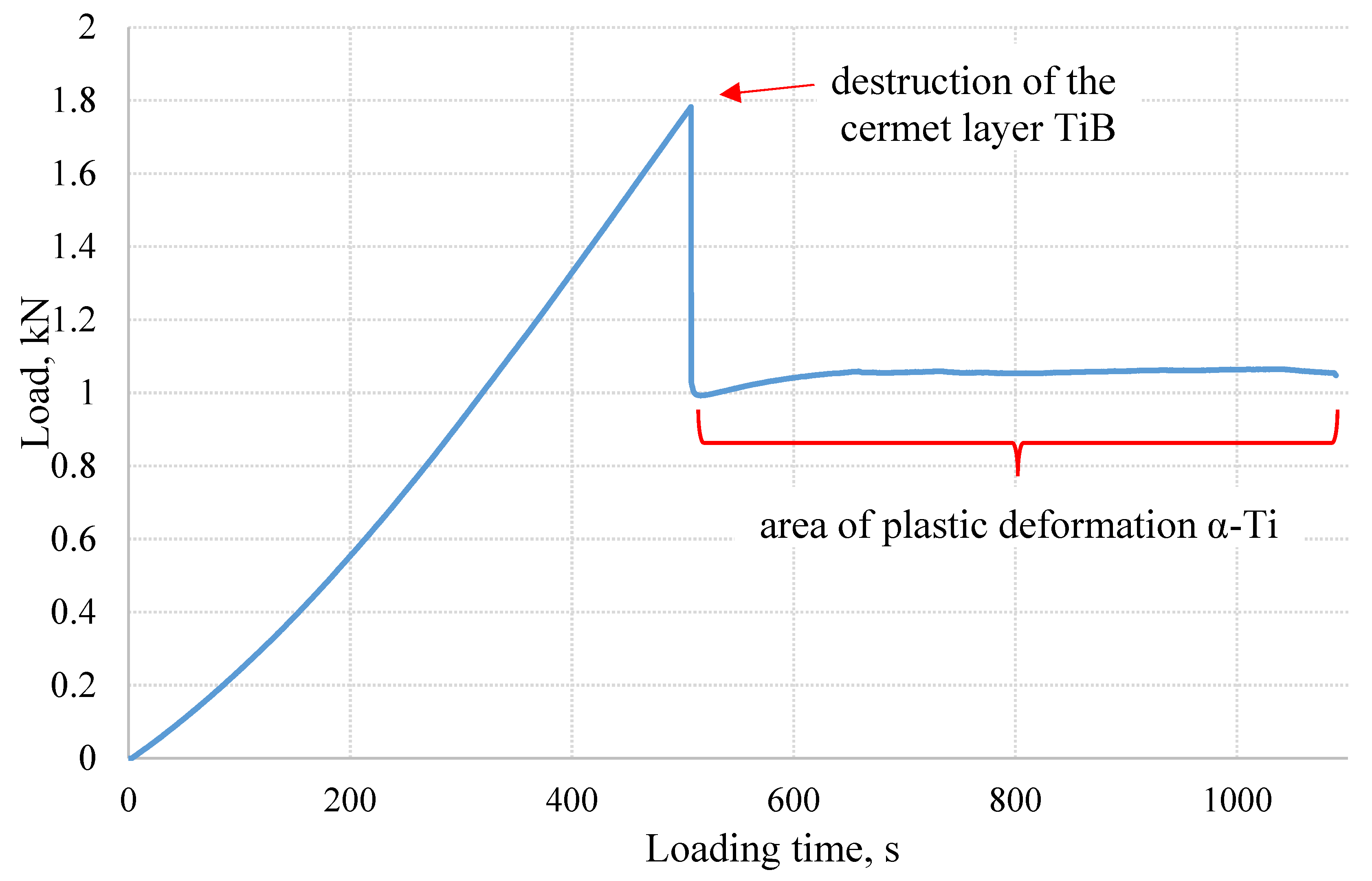
3.2. Experimental Results

As a result of the three-point bending experiments of the obtained two-layer specimens, we obtain the ultimate fracture load of the whole specimen: $P_{*}$. This is the cumulative result of the behavior of both layers as the force increases up to the limit value at which the specimen fails. The difficulty of the problem is that the different elastic properties, the proportions of the layer thicknesses, and the bending strengths mean that the failure of the specimen can be initiated either in the upper or in the lower layer. In fact, we determine the strength of one of these layers under the conditions of a two-layer stress field in the specimen.

If the value of Young’s modulus ratio parameter of both layers is determined at once, i.e., $\hspace{0.33em}\gamma =E_1/E_2$, it is then possible to choose the curve $\gamma$ of fracture order conditions of the layers (Figure 5). The area of the values of the strength ratio parameter of the layers on the ordinate axis, i.e., $\lambda ={\sigma }_1^{*}/{\sigma }_2^{*}$, above the curve $\gamma$ corresponds to the moment of the beginning of failure of the beam in the upper layer. The abscissa axis shows the thickness fraction of the bottom layer, $\eta =h/b$ (Figure 5). If we assume that brittle failure occurs without the lower layer entering plasticity, then we use relationship (13) and Figure 3. Below, we consider two typical cases and the algorithm of calculations.

3.2.1. The Bending Strength of Each Material Is Known

• We choose the material of each layer in the composite and determine (or take from the reference literature) their elastic moduli, i.e., $E_1$ and $E_2$, and obtain $\gamma =E_1/E_2$;
• We determine (or take from reference literature) the bending strength of each material separately, i.e., ${\sigma }_1^{*}$ and ${\sigma }_2^{*}$, and obtain $\lambda ={\sigma }_1^{*}/{\sigma }_2^{*}$;
• Using inequalities (13), we determine the range $\eta \in [0,{\eta }_{*})$, in which the failure occurs at the expense of the upper layer and $\eta \in [{\eta }_{*},1]$ at the expense of the lower layer.

As an example, here are the experimental results of the studied two-layer specimens with the characteristics presented in Table 1. Eight samples were studied, which were obtained with the same technological parameters of the free SHS–compression process. The samples differed in the ratio of the thicknesses of the cermet and titanium layers. The load for all samples was from the side of the cermet layer. For each specimen, three-point bending tests were performed, and the maximum forces at which the specimen failed were obtained (P_*).

Then, we obtain dimensionless parameters:

$$\gamma =E_1/E_2=0.27,\hspace{1em}\eta =h/b=0.14,\hspace{1em}\lambda ={\sigma }_{*1}/{\sigma }_{*2}=1.95$$

(35)

The equation of the curve, the finding of the parameter $\lambda$ above which corresponds to the beginning of destruction in the upper layer, and the value of the right edge ${\eta }_{*}$ of the interval at which the curve according to Equation (13) is defined $\eta \in [0,{\eta }_{*})$ are given:

$$\gamma =0.27,\hspace{1em}\lambda \left(\eta \right)=\gamma \frac{1-{\eta }^2\left(1-\gamma \right)}{{\left(1-\eta \right)}^2-{\eta }^2\gamma }=0.27\frac{1-0.73{\eta }^2}{{\left(1-\eta \right)}^2-0.27{\eta }^2},\hspace{1em}{\eta }_{*}=\frac{1}{1+\sqrt{\gamma }}=0.658,\hspace{1em}$$

(36)

Figure 5 shows us the area increase on the axis in the proportion of the thickness of the bottom layer to the whole thickness of the beam when the cause of failure is the occurrence of the first fracture in the top layer. We take into account that the plastic properties of the bottom layer leads to a decrease in stresses in it and an increase in stresses in the top layer, which stimulates its early failure.

Thus, on the basis of the calculations performed, it is established that in the three-point bending test, the destruction of the two-layer composite should start from the top layer. Indeed, when studying the structure of the specimen after the three-point bending test, it is seen that the crack is observed only in the cermet layer, and the alpha-titanium layer is not destroyed and has a clear appearance of plastic deformation (Figure 6).

The established character of specimen failure is also confirmed by the loading diagram at three-point bending. The diagram shows (as an example, the diagram for specimen S3 is given) that at 507 s, the load sharply decreased to 1 kN, which indicates the failure of the specimen. The load then increased slightly and plateaued at 1.05 kN (Figure 7). This section in the diagram indicates that the lower layer of alpha-titanium continued to undergo plastic deformation under loading.

In the graph in Figure 7, we can observe that when the load increases monotonically, it increases the load, and then, it is a sharp drop. This corresponds to brittle failure of the top layer by cracking along the vicinity of the central cross-section. In the case of a statistical deviation from the vertical axis of load application, the brittle crack returns to this vertical axis, as can be seen in Figure 6. Moreover, delamination of the beam due to the high strength of the diffusion layer does not occur in a significant range. After failure of the upper layer, at the divergence of the banks of its interface, we observe the plasticity behavior of the lower-layer material in the form of slip lines visible in Figure 6.

3.2.2. The Bending Strength of the Layer Materials Is Not Known

• We choose the material of each layer, determine (or take from reference books) their elastic moduli $E_1$ and $E_2$, and we obtain $\gamma =E_1/E_2$;
• We measure the width a and the thickness b of the sample section, the thickness of the lower layer h, and the distance between the supports L;
• We perform a three-point loading experiment on the specimen from which we obtain the value of ultimate load $P_{*}$;
• We calculate the dimensionless parameters: $l=\frac{L}{b}$, $\eta =h/b$ and cross-sectional area $S=a\cdot b$.

Depending on the observed order of layer failure, we obtain the value of the bending strength of the layer:

When the destruction began in the upper layer 2, the following is used:

$${\sigma }_{*2}\left(\gamma ,\eta \right)=\frac{3}{2}l\frac{\left({\left(1-\eta \right)}^2-\gamma {\eta }^2\right)}{\left(\gamma +\left(1-\gamma \right)\left({\left(1-\eta \right)}^4-\gamma {\eta }^4\right)\right)}\frac{P_{*}}{S}$$

(37)

When the destruction began in the lower layer 1, the following is used:

$${\sigma }_{*1}\left(\gamma ,\eta \right)=\frac{3}{2}l\gamma \frac{\left({\left(1-\eta \right)}^2-\gamma {\eta }^2\right)}{\left(\gamma +\left(1-\gamma \right)\left({\left(1-\eta \right)}^4-\gamma {\eta }^4\right)\right)}\frac{P_{*}}{S}$$

(38)

In our case, for sample S3, the failure began in the upper layer, so we use Formula (34) and obtain for $l=L/b=6$ the following:

$${\sigma }_{*2}\left(\gamma ,\eta \right)=\frac{3}{2}l\frac{\left({\left(1-\eta \right)}^2-\gamma {\eta }^2\right)}{\left(\gamma +\left(1-\gamma \right)\left({\left(1-\eta \right)}^4-\gamma {\eta }^4\right)\right)}\frac{P_{*}}{S}=632 M\Pi a$$

(39)

If we assume that the lower layer is out of plasticity during the fracture, it is worth using the inequality (34).

Let us take the values of the elastic limit ${\epsilon }_e=0.002$, the tangential modulus $E_t=2 M\Pi a$ of the upper layer, and ${\gamma }_t=E_t/E_1=2/110=0.018$.

Let us determine at what external load we can obtain the beginning of the yield to plasticity of the lower edge of the lower layer 1.

By equating the value of the maximum stress in the lower layer from Equations (11) and (26), we obtain the dependence of the bending load, above which plastic deformation in the lower layer will begin at the given elasticity limits and the value of the tangential modulus for the beam parameters from Table 1:

$$\begin{array}{l}{\sigma }_{m1}\left(\chi =\frac{1}{2},\psi =0\right)=E_1{\epsilon }_e=407\times {10}^9\times 0.002=814\times {10}^6\\ {\sigma }_{m1}=\frac{3}{2}l\gamma \frac{1+{\eta }^2\left(\gamma -1\right)}{\gamma +\left(\gamma -1\right)\left(\gamma {\eta }^4-{\left(\eta -1\right)}^4\right)}\frac{P}{S}=814 \mathrm{MPa}\\ P=2538.07\frac{\gamma +\left(\gamma -1\right)\left(\gamma {\eta }^4-{\left(\eta -1\right)}^4\right)}{\gamma +{\eta }^2\gamma \left(\gamma -1\right)}=5.932 \mathrm{kN},\hspace{1em}\gamma =0.27,\hspace{1em}\eta =0.169\end{array}$$

(40)

The resulting ultimate load for the elasticity of the lower layer is four times greater than the load at which the specimen collapsed. Thus, the specimen failure occurred in the elastic state of the lower layer, and its failure conditions are reliably described by the relationship (13).

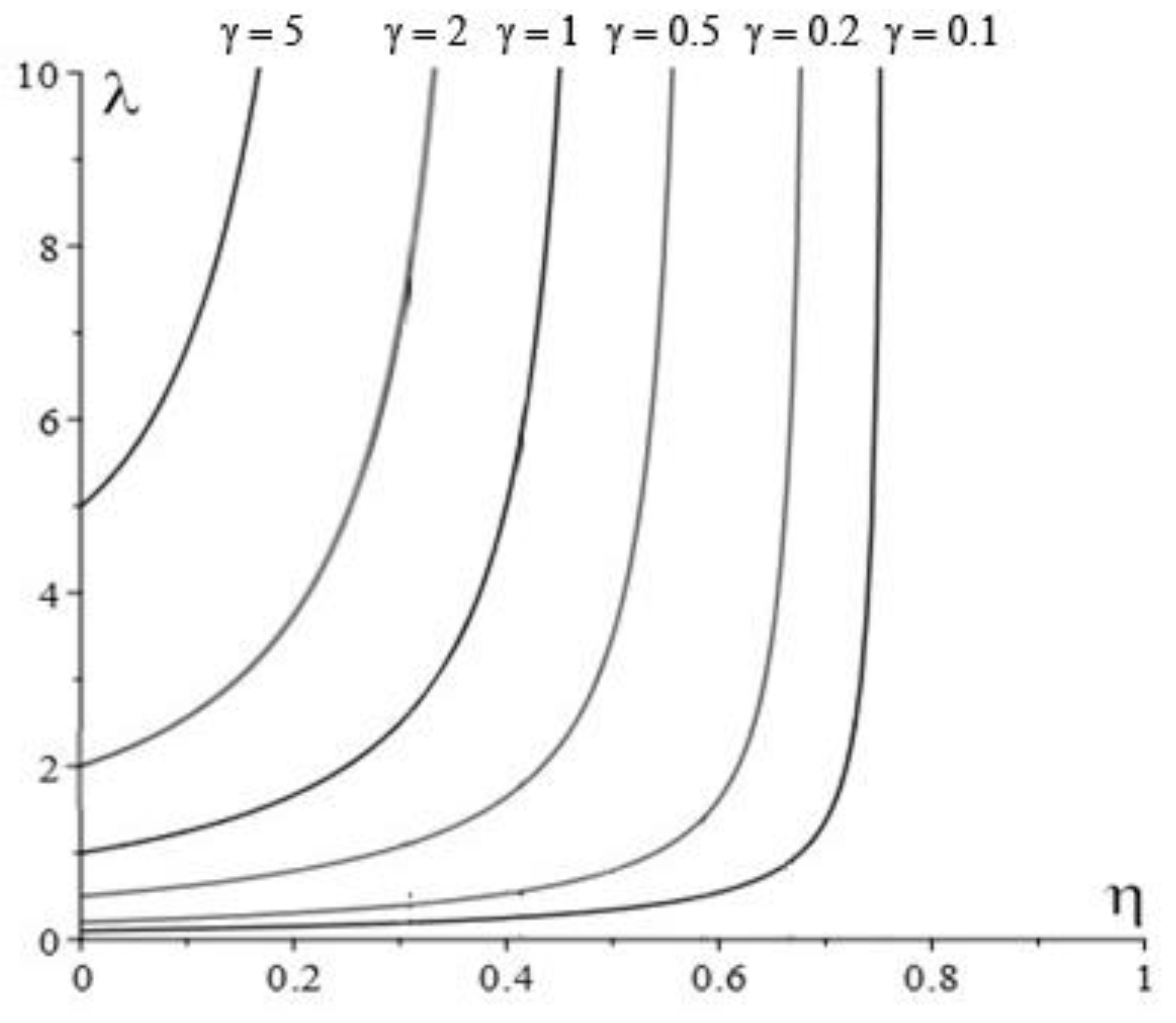
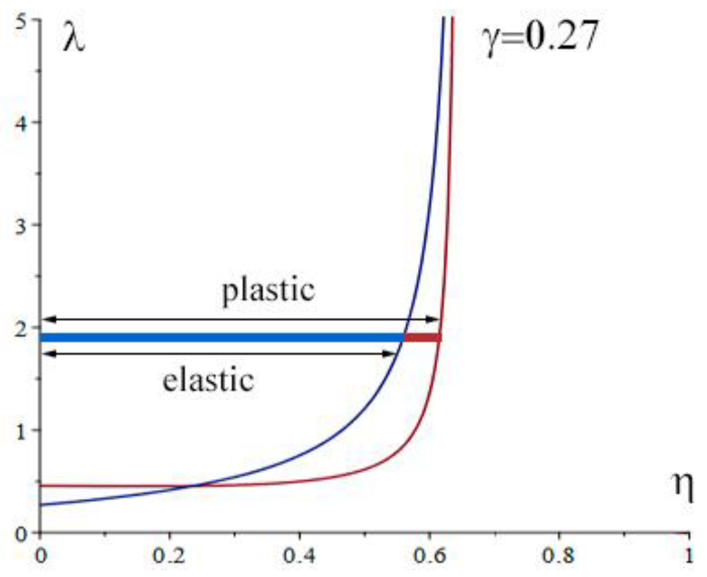
3.3. Maximum Load Setting

Let us find the maximum load that can be applied to a two-layer specimen given the proportion of Young’s moduli, i.e., $\gamma =E_1/E_2=0.27$, and the bending strength limits of the upper and lower layers, $\lambda ={\sigma }_1^{*}/{\sigma }_2^{*}=1.95$.

If the neutral axis passes through the top layer, $0<\eta <1/\left(1+\sqrt{\gamma }\right)$. In this case, the destruction will occur in the upper layer under the condition (13), from which we obtain the following:

$0<\eta <0.658$.

Then, let us express the magnitude of the load P from Equation (10):

$$P=\frac{2{\sigma }_{*2}S}{3l}\frac{\left(\gamma +\left(1-\gamma \right)\left({\left(1-\eta \right)}^4-\gamma {\eta }^4\right)\right)}{{\left(1-\eta \right)}^2-\gamma {\eta }^2}$$

(41)

and this load is a monotonically increasing function for the area $\eta \in \left(0.19,0.658\right)$.

Failure will occur in the lower layer at $\eta >0.658$.

And ultimate load for the lower layer breakage case will be from Equation (11):

$$P=\frac{2{\sigma }_{*1}S}{3\gamma l}\frac{\left(\gamma +\left(1-\gamma \right)\left({\left(1-\eta \right)}^4-\gamma {\eta }^4\right)\right)}{1+{\eta }^2\left(\gamma -1\right)}$$

(42)

But, if we compare ultimate loads for the area $\eta <0.658$, we can find the branch where ultimate load for the lower layer is smaller and then for the upper layer. And we can find the condition for the maximum available ultimate load:

$$\eta =\frac{\sqrt{\gamma \left({\lambda }^2-{\gamma }^2\right)+{\gamma }^2}-\lambda }{\left(\gamma -1\right)\left(\gamma +\lambda \right)}=0.562$$

(43)

As a result, we obtain the dependence of the destructive load at given strengths and Young’s moduli, as shown in Figure 8.

The red curve corresponds to the case when the failure in the upper layer occurs at a lower load than in the lower layer. Then, this dependence of the ultimate load on the proportion of the thickness of the bottom layer to the whole thickness of the beam increases, while the ultimate load for failure of the bottom layer monotonically decreases. And already, the right blue part of the curve corresponds to the case of the first failure of the bottom layer.

From the presented Figure 8, it is shown that the experimental results are in good agreement with the theoretical results. Thus, it is possible to assert the adequacy of the developed mathematical model. It can also be seen that in order to increase the maximum load for the destruction of two-layer samples, it is necessary to use samples with a thickness ratio closer to 0.6. A further increase in the ratio of layer thicknesses does not lead to a significant change in the ultimate load. Starting with a layers thickness ratio of 0.8, the load decreases sharply. In this case, this is due to a decrease in the thickness of the cermet layer.

The maximum ultimate load for three-point bending test will be achieved for the dimensionless size of bottom-layer thickness:

$${\eta }_m=\frac{\sqrt{\gamma \left({\lambda }^2-{\gamma }^2\right)+{\gamma }^2}-\lambda }{\left(\gamma -1\right)\left(\gamma +\lambda \right)},\hspace{1em}{P}_{\max }=\frac{2{\sigma }_{*1}S}{3\gamma l}\frac{\left(\gamma +\left(1-\gamma \right)\left({\left(1-{\eta }_m\right)}^4-\gamma {\eta }_m{}^4\right)\right)}{1+{\eta }_m{}^2\left(\gamma -1\right)}$$

(44)

4. Conclusions

We are able to predict in advance which layer, based on the three bilayer parameters of $\eta ,\gamma ,\lambda$, will trigger the brittle fracture mechanism for elastic properties of both layers (13). When we consider plasticity of bottom layer, we can use Equation (26). Accordingly, the dependence of the external load on the strength of which layer material is worth considering when determining the strength of the entire two-layer material.

In the case that $\lambda$ is above the graph (Figure 2), we can obtain from a three-point bending test of the two-layered beam the flexural strength of the upper layer 2 material ${\sigma }_{*2}$, according to the given parameters of the two-layer material and the value of the ultimate load $P_{*}$ with the aid of Equation (39).

In the case that $\lambda$ is under the graph (Figure 2), we obtain the bending strength for the bottom layer 1 ${\sigma }_{*1}$, according to the given parameters of the two-layer material and the value of the ultimate load $P_{*}$ with the aid of Equation (38).

The main conclusion of the work is the possibility to increase the minimum three-point bending ultimate load $P_{*}$ of the two-layer beam (1500 MPa) by a factor of three (4500 MPa) when choosing the thickness of the bottom layer of the order of 60% of the total thickness (Figure 7) for the case $\gamma =E_1/E_2=0.27$ and $\lambda ={\sigma }_1^{*}/{\sigma }_2^{*}=1.95$.

If the thickness of the bottom layer is not less than in Equation (43), the ultimate load limit will be determined by the bending strength of the bottom layer. Otherwise, we also must consider the strength of the top layer.

Equation (44) sets the conditions and values for the maximum load achievement.

References

1. Wei, J.; Yang, F.; Zhang, C.; Chen, C.; Guo, Z. The “Pinning” Effect of in-Situ TiB Whiskers on the Hot Deformation Behavior and Dynamic Recrystallization of (10 Vol%) TiB/Ti–6Al–4V Compos. J. Mater. Res. Technol. 2023, 22, 1695–1707. [Google Scholar] [CrossRef]
2. Li, S.; Han, Y.; Shi, Z.; Huang, G.; Zong, N.; Le, J.; Qiu, P.; Lu, W. Synergistic Strengthening Behavior and Microstructural Optimization of Hybrid Reinforced Titanium Matrix Composites during Thermomechanical Processing. Mater. Charact. 2020, 168, 110527. [Google Scholar] [CrossRef]
3. Jeje, S.O.; Shongwe, M.B.; Rominiyi, A.L.; Olubambi, P.A. Spark Plasma Sintering of Titanium Matrix Composite—A Review. Int. J. Adv. Manuf. Technol. 2021, 117, 2529–2544. [Google Scholar] [CrossRef]
4. Zhou, Y.; Yang, F.; Chen, C.; Shao, Y.; Lu, B.; Sui, Y.; Guo, Z. Mechanical Property and Microstructure of In-Situ TiB/Ti Composites via Vacuum Sintering and Hot Rolling. J. Alloys Compd. 2022, 911, 165042. [Google Scholar] [CrossRef]
5. Liang, S.; Li, W.; Jiang, Y.; Cao, F.; Dong, G.; Xiao, P. Microstructures and Properties of Hybrid Copper Matrix Composites Reinforced by TiB Whiskers and TiB2 Particles. J. Alloys Compd. 2019, 797, 589–594. [Google Scholar] [CrossRef]
6. Bagliuk, G.A.; Stasiuk, A.A.; Savvakin, D.G. Effect of Titanium Diboride Content on Basic Mechanical Properties of Composites Sintered from TiH2+ TiB2 Powder Mixtures. Powder Metall. Met. Ceram. 2020, 58, 642–650. [Google Scholar] [CrossRef]
7. Tan, D.-W.; Chen, Z.-W.; Wei, W.-X.; Song, B.-C.; Guo, W.-M.; Lin, H.-T.; Wang, C.-Y. Wear Behavior and Mechanism of TiB2-Based Ceramic Inserts in High-Speed Cutting of Ti6Al4V Alloy. Ceram. Int. 2020, 46, 8135–8144. [Google Scholar] [CrossRef]
8. Huang, K.; Chen, W.; Wu, M.; Wang, J.; Jiang, K.; Liu, J. Microstructure and Densification of the Ti6Al4V–70% TiB2 Metal-Ceramic by Coupled Multi-Physical Fields-Activated Sintering. J. Alloys Compd. 2020, 820, 153091. [Google Scholar] [CrossRef]
9. Yang, H.-Y.; Wang, Z.; Yue, X.; Ji, P.-J.; Shu, S.-L. Simultaneously Improved Strength and Toughness of In Situ Bi-Phased TiB2–Ti (C, N)–Ni Cermets by Mo Addition. J. Alloys Compd. 2020, 820, 153068. [Google Scholar] [CrossRef]
10. Han, J.; Liu, Z.; Jia, Y.; Wang, T.; Zhao, L.; Guo, J.; Xiao, S.; Chen, Y. Effect of TiB2 Addition on Microstructure and Fluidity of Cast TiAl Alloy. Vacuum 2020, 174, 109210. [Google Scholar] [CrossRef]
11. Ozerov, M.; Klimova, M.; Sokolovsky, V.; Stepanov, N.; Popov, A.; Boldin, M.; Zherebtsov, S. Evolution of Microstructure and Mechanical Properties of Ti/TiB Metal-Matrix Composite during Isothermal Multiaxial Forging. J. Alloys Compd. 2019, 770, 840–848. [Google Scholar] [CrossRef]
12. Zhang, T.; Zhao, N.; Shi, C.; He, C.; Liu, E. Regulation of the Interface Binding and Mechanical Properties of TiB/Ti via Doping-Induced Chemical and Structural Effects. Comput. Mater. Sci. 2020, 174, 109506. [Google Scholar] [CrossRef]
13. Lin, Y.; Lin, Z.; Chen, Q.; Lei, Y.; Fu, H. Laser In-Situ Synthesis of Titanium Matrix Composite Coating with TiB–Ti Network-like Structure Reinforcement. Trans. Nonferrous Met. Soc. China 2019, 29, 1665–1676. [Google Scholar] [CrossRef]
14. Zhao, S.; Xu, Y.; Pan, C.; Liang, L.; Wang, X. Microstructural Modeling and Strengthening Mechanism of TiB/Ti-6Al-4V Discontinuously-Reinforced Titanium Matrix Composite. Materials 2019, 12, 827. [Google Scholar] [CrossRef]
15. Xueqiao, L.; Tounan, J.; Shejun, D.; Lei, C.; Yinghua, L.; Yongping, L. Formation Mechanism of the Tubular TiB In Situ Formed in TiB/Ti-6Al-4V Composite Coatings by Laser Cladding. Rare Met. Mater. Eng. 2018, 47, 915–919. [Google Scholar]
16. Jianwei, M.; Guangfa, H.; Liqiang, W.; Yuanfei, H.; Weijie, L. Microstructural Evolutions of In-Situ TiB Whisker Reinforcement during Laser Welding TiB/Ti Composites. Rare Met. Mater. Eng. 2017, 46, 112–117. [Google Scholar]
17. Selvakumar, M.; Ramkumar, T.; Mohanraj, M.; Chandramohan, P.; Narayanasamy, P. Experimental Investigations of Reciprocating Wear Behavior of Metal Matrix (Ti/TiB) Composites. Archiv. Civ. Mech. Eng. 2020, 20, 26. [Google Scholar] [CrossRef]
18. Konstantinov, A.S.; Bazhin, P.M.; Stolin, A.M.; Kostitsyna, E.V.; Ignatov, A.S. Ti-B-Based Composite Materials: Properties, Basic Fabrication Methods, and Fields of Application. Compos. Part A. 2018, 108, 79–88. [Google Scholar] [CrossRef]
19. Wang, S.; Huang, L.; Zhang, R.; An, Q.; Sun, F.; Meng, F.; Geng, L. Effects of Rolling Deformation on Microstructure Orientations and Tensile Properties of TiB/(TA15-Si) Composites. Mater. Charact. 2022, 194, 112425. [Google Scholar] [CrossRef]
20. Hasan, M.; Zhao, J.; Jiang, Z. Micromanufacturing of Composite Materials: A Review. Int. J. Extrem. Manuf. 2019, 1, 012004. [Google Scholar] [CrossRef]
21. Huang, M.; Xu, C.; Fan, G.; Maawad, E.; Gan, W.; Geng, L.; Lin, F.; Tang, G.; Wu, H.; Du, Y.; et al. Role of Layered Structure in Ductility Improvement of Layered Ti-Al Metal Composite. Acta Mater. 2018, 153, 235–249. [Google Scholar] [CrossRef]
22. Bazhin, P.M.; Konstantinov, A.S.; Chizhikov, A.P.; Pazniak, A.I.; Kostitsyna, E.V.; Prokopets, A.D.; Stolin, A.M. Laminated Cermet Composite Materials: The Main Production Methods, Structural Features and Properties (Review). Ceram. Int. 2021, 47, 1513–1525. [Google Scholar] [CrossRef]
23. Wan, H.; Leung, N.; Jargalsaikhan, U.; Ho, E.; Wang, C.; Liu, Q.; Peng, H.-X.; Su, B.; Sui, T. Fabrication and Characterisation of Alumina/Aluminium Composite Materials with a Nacre-like Micro-Layered Architecture. Mater. Des. 2022, 223, 111190. [Google Scholar] [CrossRef]
24. Charkviani, R.V.; Pavlov, A.A.; Pavlova, S.A. Interlaminar Strength and Stiffness of Layered Composite Materials. Procedia Eng. 2017, 185, 168–172. [Google Scholar] [CrossRef]
25. Cao, Z.H.; Sun, W.; Ma, Y.J.; Li, Q.; Fan, Z.; Cai, Y.P.; Zhang, Z.J.; Wang, H.; Zhang, X.; Meng, X.K. Strong and Plastic Metallic Composites with Nanolayered Architectures. Acta Mater. 2020, 195, 240–251. [Google Scholar] [CrossRef]
26. Mo, T.; Chen, J.; Chen, Z.; He, W.; Liu, Q. Microstructure Evolution During Roll Bonding and Growth of Interfacial Intermetallic Compounds in Al/Ti/Al Laminated Metal Composites. JOM 2019, 71, 4769–4777. [Google Scholar] [CrossRef]
27. Ma, M.; Huo, P.; Liu, W.C.; Wang, G.J.; Wang, D.M. Microstructure and Mechanical Properties of Al/Ti/Al Laminated Composites Prepared by Roll Bonding. Mater. Sci. Eng. 2015, 636, 301–310. [Google Scholar] [CrossRef]
28. Nasakina, E.O.; Sudarchikova, M.A.; Demin, K.Y.; Gol’Dberg, M.A.; Baskakova, M.I.; Tsareva, A.M.; Ustinova, Y.N.; Leonova, Y.O.; Sevost’yanov, M.A. The Effect of the Titanium Surface Layer Thickness on the Characteristics of a Layered Composite Material. Proc. J. Phys. Conf. Ser. IOP Publ. 2019, 1281, 012057. [Google Scholar] [CrossRef]
29. Chen, Z.; Zheng, Y.; Löfler, L.; Bartosik, M.; Nayak, G.K.; Renk, O.; Holec, D.; Mayrhofer, P.H.; Zhang, Z. Atomic Insights on Intermixing of Nanoscale Nitride Multilayer Triggered by Nanoindentation. Acta Mater. 2021, 214, 117004. [Google Scholar] [CrossRef]
30. Prokopets, A.D.; Bazhin, P.M.; Konstantinov, A.S.; Chizhikov, A.P.; Antipov, M.S.; Avdeeva, V.V. Structural Features of Layered Composite Material TiB2/TiAl/Ti6Al4 Obtained by Unrestricted SHS-Compression. Mater. Lett. 2021, 300, 130165. [Google Scholar] [CrossRef]
31. Song, K.; Xu, Y.; Zhao, N.; Zhong, L.; Shang, Z.; Shen, L.; Wang, J. Evaluation of Fracture Toughness of Tantalum Carbide Ceramic Layer: A Vickers Indentation Method. J. Mater. Eng. Perform. 2016, 25, 3057–3064. [Google Scholar] [CrossRef]
32. Du, W.; Han, B.; Li, X.; Wu, H.; Miao, K.; Li, R.; Wu, H.; Liu, C.; Fang, W.; Fan, G. Fracture Mechanism of High Toughness Ti2AlNb/Ti6Al4V Layered Metal Composites. Mater. Lett. 2023, 348, 134717. [Google Scholar] [CrossRef]
33. Wu, H.; Fan, G.; Jin, B.C.; Geng, L.; Cui, X.; Huang, M.; Li, X.; Nutt, S. Enhanced Fracture Toughness of TiBw/Ti3Al Composites with a Layered Reinforcement Distribution. Mater. Sci. Eng. 2016, 670, 233–239. [Google Scholar] [CrossRef]
34. Ladeveze, P.; LeDantec, E. Damage Modelling of the Elementary Ply for Laminated Composites. Compos. Sci. Technol. 1992, 43, 257–267. [Google Scholar] [CrossRef]
35. Polilov, A.N.; Sklemina, O.Y. Delamination of Composites and the Scale Effect of Glued Joint Strength. Polym. Sci. Ser. D 2023, 16, 104–110. [Google Scholar] [CrossRef]
36. Williams, K.V.; Vaziri, R.; Poursartip, A. A Physically Based Continuum Damage Mechanics Model for Thin Laminated Composite Structures. Int. J. Solids Struct. 2003, 40, 2267–2300. [Google Scholar] [CrossRef]
37. Vasiliev, V.V.; Morozov, E.V. Chapter 7—Laminated Composite Plates. In Advanced Mechanics of Composite Materials and Structures, 4th ed.; Vasiliev, V.V., Morozov, E.V., Eds.; Elsevier: Amsterdam, The Netherlands, 2018; pp. 437–574. ISBN 978-0-08-102209-2. [Google Scholar] [CrossRef]
38. McCartney, L.N. Physically Based Damage Models for Laminated Composites. Proc. Inst. Mech. Eng. 2003, 217, 163–199. [Google Scholar] [CrossRef]
39. Öchsner, A. Classical Beam Theories of Structural Mechanics/eBook: Physics and Astronomy; Springer: New York City, NY, USA, 2021. [Google Scholar] [CrossRef]
40. Bazhina, A.D.; Chizhikov, A.; Konstantinov, A.; Khomenko, N.; Bazhin, P.; Avdeeva, V.; Chernogorova, O.; Drozdova, E. Structure, Phase Composition and Mechanical Characteristics of Layered Composite Materials Based on TiB/XTi-Al/α-Ti (x = 1, 1.5, 3) Obtained by Combustion and High-Temperature Shear Deformation. Mater. Sci. Eng. 2022, 858, 144161. [Google Scholar] [CrossRef]
41. Bazhin, P.; Konstantinov, A.; Chizhikov, A.; Prokopets, A.; Bolotskaia, A. Structure, Physical and Mechanical Properties of TiB-40 Wt.%Ti Composite Materials Obtained by Unrestricted SHS Compression. Mater. Today Commun. 2020, 25, 101484. [Google Scholar] [CrossRef]
42. Ding, H.; Cui, X.; Gao, N.; Sun, Y.; Zhang, Y.; Huang, L.; Geng, L. Fabrication of (TiB/Ti)-TiAl composites with a controlled laminated architecture and enhanced mechanical properties. J. Mater. Sci. Technol. 2021, 62, 221–233. [Google Scholar] [CrossRef]
43. Zhong, Z.; Zhang, B.; Jin, Y.; Zhang, H.; Wang, Y.; Ye, J.; Liu, Q.; Hou, Z.; Zhang, Z.; Ye, F. Design and anti-penetration performance of TiB/Ti system functionally graded material armor fabricated by SPS combined with tape casting. Ceram. Int. 2020, 46, 28244–28249. [Google Scholar] [CrossRef]
44. Lapshin, O.V.; Boldyreva, E.V.; Boldyrev, V.V. Role of Mixing and Milling in Mechanochemical Synthesis (Review). Russ. J. Inorg. Chem. 2021, 66, 433–453. [Google Scholar] [CrossRef]
45. Tomilin, O.B.; Muryumin, E.E.; Fadin, M.V.; Shchipakin, S.Y. Preparation of Luminophore CaTiO3:Pr3+ by Self-Propagating High-Temperature Synthesis. Russ. J. Inorg. Chem. 2022, 67, 431–438. [Google Scholar] [CrossRef]
46. Bazhin, P.M.; Chizhikov, A.P.; Konstantinov, A.S.; Prokopets, A.D.; Kostitsyna, E.V.; Bolotskaya, A.V.; Stolin, A.M.; Khomenko, N.Y. TiB/30 wt.% Ti layered composite material obtained by free SHS compression on a Ti6Al4V titanium alloy. IOP Conf. Ser. Mater. Sci. Eng. 2020, 848, 012009. [Google Scholar] [CrossRef]
47. Bazhin, P.M.; Stolin, A.M.; Konstantinov, A.S.; Chizhikov, A.P.; Prokopets, A.D.; Alymov, M.I. Structural Features of Titanium Boride-Based Layered Composite Materials Produced by Free SHS Compression. Dokl. Chem. 2019, 488, 246–248. [Google Scholar] [CrossRef]
48. Chizhikov, A.; Konstantinov, A.; Bazhin, P.; Stolin, A. Features of Molding and Structure of Composite Materials Based on TiB/Ti, Obtained by Free SHS Compression Method. Mater. Sci. Forum. 1009, 2020, 37–42. [Google Scholar] [CrossRef]
49. Stolin, A.M.; Bazhin, P.M.; Konstantinov, A.S.; Alymov, M.I. Production of Large Compact Plates from Ceramic Powder Materials by Unconfined SHS Compaction. Dokl. Chem. 2018, 480, 136–138. [Google Scholar] [CrossRef]
50. Bazhin, P.M.; Stolin, A.M.; Konstantinov, A.S.; Kostitsyna, E.V.; Ignatov, A.S. Ceramic Ti—B Composites Synthesized by Combustion Followed by High-Temperature Deformation. Materials 2016, 9, 1027. [Google Scholar] [CrossRef]
Figure 1. Schematic diagram of the beam: green—cermet TiB/Ti layer, grey—α-Ti.
Metals 13 01480 g001
Figure 2. Schematic of the experiment method by free SHS compression.
Metals 13 01480 g002
Figure 3. Boundaries of the fracture sequence of layers. Upper layer breaks first when is over the curve for certain γ .
Metals 13 01480 g003
Figure 4. Dependence of the ratio of the maximum tensile stress to the fracture stress component along the psi axis.
Metals 13 01480 g004
Figure 5. Sample points S1–S8 are in the zone of the beginning of destruction of the upper layer in both elastic (blue bar) and plastic (blue and red bar) cases.
Metals 13 01480 g005
Figure 6. Crack propagation in specimen No. S3: (a) macro image of LCM and cracks, (b) top layer, (c) border cermet layer TiB/Ti—α-Ti.
Metals 13 01480 g006
Figure 7. Load diagram of specimen No. S3.
Metals 13 01480 g007
Figure 8. Dependence of the maximum load on the ratio of the thickness of the bottom layer to the whole thickness of the beam and the experimental data for samples No. S1–S8.
Metals 13 01480 g008