
An Investigation of Spiral Dislocation Sources Using Discrete Dislocation Dynamics (DDD) Simulations
Department of Mechanical Engineering, University of New Mexico, Albuquerque, NM 87131, USA
*
Author to whom correspondence should be addressed.
Metals 2023, 13(8), 1408; https://doi.org/10.3390/met13081408
Submission received: 12 July 2023
/
Revised: 2 August 2023
/
Accepted: 4 August 2023
/
Published: 6 August 2023
(This article belongs to the Special Issue Deformation of Metals and Alloys: Theory, Simulations and Experiments)
Abstract
:Discrete Dislocation Dynamics (DDD) simulations are a powerful simulation methodology that can predict a crystalline material’s constitutive behavior based on its loading conditions and micro-constituent population/distribution. In this paper, a 3D DDD model with spiral dislocation sources is developed to study size-dependent plasticity in a pure metal material (taken here as Aluminum). It also shows, for the first time, multipole simulations of spirals and how they interact with one another. In addition, this paper also discusses how the free surface of a crystalline material affects the plasticity generation of the spiral dislocation. The surface effect is implemented using the Distributed Dislocation Method. One of the main results from this work, shown here for the first time, is that spiral dislocations can result in traditional Frank–Read sources (edge or screw character) in a crystal. Another important result from this paper is that with more dislocation sources, the plastic flow inside the material is more continuous, which results in a lowering of the flow stress. Lastly, the multipole interaction of the spiral dislocations resulted in a steady-state fan-shaped action for these dislocation sources.
1. Introduction
Material defects usually form due to the disequilibrium conditions of manufacturing processes and environmental effects. Point, line, surface, and volume defects are four of the main types of defects that exist in materials. Dislocations are line defects that represent an extra half plane (edge dislocation) in the crystal or a shifted half plane in the three-dimensional atomic array of a crystal [1]. In addition to dislocations being generated from the above effects, dislocations in a crystal can be generated from dislocation sources. There are two main dislocation sources in a crystal: Frank–Read (FR) sources and spiral dislocation sources. An FR source is a dislocation line strongly pinned at two end points of the dislocation (see Figure 1a) [1,2]. A spiral dislocation source is formed when a dislocation has a single fixed point on its slip plane (see Figure 1b) [1,2]. The other end of the dislocation is at a free surface or a grain boundary.
In the mid-20th century, the configuration of a spiral source in a silicon bar twisted at 900 Celsius was elucidated using 3D X-ray projection topographs [3]. Later, spiral dislocation sources were captured and observed in a Terrace Ledge Kink model, which fully demonstrated the kinetics of low-index crystal surface evaporation [4]. In quantum systems, a spiral dislocation in an elastic medium was used to analyze its influence on the harmonic oscillator. A new contribution to the energy level of a harmonic oscillator interacting with a quantum particle was found to be affected by spiral dislocations [5]. A similar study was performed by Maia et al.: the Landau levels, which are energy levels of charged particles in a magnetic field, were modified even though there was no interaction between electrons and the spiral dislocation [6]. A new way that scatters electrons in a lattice structure around a spiral dislocation has been developed by Kiyoshi [7].
Furthermore, 3D DDD simulations with a spiral dislocation source were utilized to explain the dependence of the strength of thin films on the film thickness. Validation of the simulation data has been performed, and it was found that the yield strength of the thin film is inversely proportional to the film thickness [8].
Three-dimensional Discrete Dislocation Dynamics (DDD) is a simulation methodology utilized to capture the behavior and interaction of finite curved dislocations. In the early stages of DDD, the model was two-dimensional, and the infinitely long line dislocations could only be edge dislocations or screw dislocations [9,10,11,12]. A study of plastic deformation taken to occur by the motion of edge dislocations in a single crystal thin film was demonstrated using the 2D discrete dislocation dynamics method [13]. The 2D DDD simulations, confined to a single slip system and to the collective behavior of edge dislocations, were utilized to investigate the grain size effect on material strengthening [14].
Later on, DDD modeling was improved by Kubin and associates [15], followed by Zbib and associates [16,17,18] as well as other researchers [19,20].
After the improvement, the model can discretize curved dislocations into mixed dislocation segments, which means the dislocation segments have the characters of edge dislocations and screw dislocations. Three-dimensional DDD can capture long-range and short-range interactions of tortuous dislocations in differently shaped computational domains. In this model, the dislocation segments move under the influence of internal or external stresses using some sort of a time-marching scheme.
In the current study, 3D DDD simulations are utilized to elucidate the size–scale effect on the plastic behavior of a spiral dislocation source. This is very important for situations with confined spaces or dimensions, such as thin films or quantum dots. In addition, this particularly work shows for the first time how spiral dislocations can form traditional Frank–Read sources and the interaction of multipoles. Moreover, the Distributed Dislocation Method (DDM) is used to investigate the free surface effects in DDD simulations for a spiral dislocation source. The basic idea of DDM is to mesh a surface with dislocation loops in order to ensure or enforce the traction-free boundary condition of the free surface at a set of collocation surface points. Fundamental dislocation solutions used in DDM have been developed with the aid of the stress field expressions for straight dislocation segments provided by Devincre [21]. The investigation of free-surface effects in 3D dislocation dynamics has been performed by Khraishi et al. [22,23,24,25].
2. Method
In dislocation dynamics, continuously curved dislocation lines are estimated with connected straight dislocation segments, which is also known as a discretization step. The premise of this discretization step is that the self-stress of the originally curved dislocations can be obtained from summing the self-stresses of the discrete linear dislocation segments. The self-stress of straight dislocation lines in an infinite medium has been developed and presented previously in the literature [1,2]. The stress field associated with a dislocation segment has been given by Hirth et al [2] for an intrinsic or segment-attached coordinate system, and by Devincre [21] for any coordinate system. It is a main component applied to calculating the Peach–Koehler force and total stress felt by a dislocation segment in dislocation dynamics codes. The Peach–Koehler force is a force produced by external stresses to the linear dislocation segment. The Peach–Koehler force on a segment that can capture the mutual interaction of discrete linear dislocation segments is given by the following [16]:
where “” represents multiplication, “” stands for the cross product, (note that a bolded parameter represents a vector in this paper) is the Burgers vector, is the line sense, and and are self-forces from the immediate neighboring dislocation segments. is the total stress acting at the center of segment , as follows:
where is self-stress from other dislocation segments besides segment or the two immediate neighboring segments, is the stress from externally applied loads, and is the stress emanating from other sources such as cracks, free surfaces, eigenstrain fields, etc.
The Peach–Koehler force calculated from Equation (1) can be used to develop velocities of dislocation segments [17]:
where is the glide velocity, is the dislocation mobility, and is the glide component of the Peach–Koehler force .
The motion of a dislocation segment is determined by the Peach–Koehler force. If the Peach–Koehler force is able to overcome hindrances in the lattice, dislocation segments can expand and move continuously. Nodal velocities of segments can be obtained since the glide velocity of a segment can be calculated using Equation (3). To be specific, the nodal velocity is obtained by averaging two adjacent segments’ velocities. Note that each segment has two nodes, as Figure 2 shows, and two adjacent segments share one node. Consequently, the plastic strain rate for the computational cell or domain can be developed using the following equation [16]:
where is the jth segment length, is the unit normal vector of the slip plane, is the Burgers vector of the dislocation segment, and is the volume of the simulated crystal/computational cell/domain.
With the plastic strain rate, the stress increment of the computational cell can be evaluated over a time increment [17]:
where is the Young’s modulus, is the total strain rate in the loading direction, and (where is the elastic strain and is the plastic strain). Then, the constitutive behavior of the material can be captured by the stress–strain curve.
For the DDD simulation of a traditional FR source (Figure 1a), a simulation box with dimensions 60,000b × 60,000b × 40,000b is centered on the cartesian coordinate origin. The FR source is placed along the x-axis with one end fixed at the nodal point (−15,000b, 0, 0) and the other end fixed at (15,000b, 0, 0), where b is the magnitude of the Burgers vector (equal to 0.286 [nm]). The direction of the Burgers vector is (0, 1, 0). The following parameters are used for the DDD simulation of the traditional FR source: The dislocation mobility (): 10,000 [1/(Pa·s)]; The material properties of Aluminum are used: the shear modulus (G) and Poisson’s ratio () are 26.32 [GPa] and 0.33, respectively. The applied constant shear strain rate is equal to 10 [s−1]. The minimum segment length is equal to 300b. The total source length (L) is equal to 30,000b. The minimum time step is equal to 10−12 [s]. The result of this simulation is presented in Figure 3. It is observed in the figure that the stress–strain curve starts linear with elastic deformation and then reaches a proportional limit (initial yielding [23]) followed eventually by a steady state of plasticity generation (the average stress value of which is termed the “flow stress” or ).
3. Simulation Results and Discussion
3.1. Spiral Dislocation Configuration in a Large Simulation Box (without Surface Effect)
The first 3D DDD simulations focus on two scenarios: (1) a spiral dislocation source extending from the center of the simulation box to the free surface (Figure 4a, which is similar to Figure 1b) and (2) a spiral dislocation source similar to scenario #1 but also having an extended dislocation line from the center of the box to the top surface of the box (Figure 4b). Scenario #2 was implemented in accordance with standard textbooks (e.g., [1,2]), which points to dislocations not terminating in the middle of a crystal anywhere but rather at free surfaces or other internal surfaces.
The purpose of these two scenarios is two-fold: (1) to show if the extended dislocation line lying along the z-axis will have any effect on the initial (i.e., time zero) equilibrium of the source, and (2) on the dynamic equilibrium of the source and especially the ensuing stress–strain curve from an applied strain rate. The dislocation motion results of running scenario 1 are shown in Figure 4a–c. Each of which shows a snapshot in time or for a specific applied strain value. The dislocation motion results of running scenario 2 are shown in Figure 4b,d,f.
The results of running these two scenarios are as follows. First off, having the initial configuration in Figure 4a/Figure 1b does not affect the initial static equilibrium of the source. This is similar to a typical FR source (Figure 1a), which has been run as such in many previous works (e.g., [24,26]) (see Figure 3). Moreover, having the extended dislocation in scenario (2) also does not affect the initial static equilibrium of the spiral source. Another result, which is shown in Figure 4e,f, is that the motion of the glissile dislocations (the ones lying in the xy-plane in this case) is not affected by the presence or use of an extended dislocation lying along the z-axis (scenario 2) versus the absence of such extended dislocation (scenario 1). Notice that the extended dislocation in scenario 2 is not on a slip plane and, hence, stays stationary through the operation of the spiral source. In this section, the authors used a large simulation box to show more circles of the spiral dislocation source. However, running the simulation in a large simulation box is extremely time-consuming. Therefore, a relatively small simulation box is used in the rest of this work.
3.2. DDD Simulations for the Study of Size–Scale Effect (without Surface Effect)
In the literature, the effect of size–scale effects have been well documented as it affects things like the strength of the material (see the following references for example: [8,27,28,29,30]). In this section, the authors shed light on the cause of such changes in the strength of a crystal, specifically its flow stress, with changes in the crystal dimensions. Such a study was never performed before using a spiral dislocation source (to the authors’ knowledge). Here, a simulation box with dimensions S1 × S2 × S3 is centered on the cartesian coordinate origin for all simulations. A spiral dislocation source is placed along the x-axis with one end fixed at the nodal point (0, 0, 0) and the other end fixed at (30,000b = S1/2, 0, 0), where b is the magnitude of the Burgers vector (equal to 0.286 [nm]). The direction of the Burgers vector is (0, 1, 0). The dislocation mobility () used in the simulations is 10,000 [1/(Pa*s)]. The Shear modulus (G) and Poisson’s ratio () are 26.32 [GPa] and 0.33, respectively (Aluminum). In addition to the above parameters, the following ones are used to obtain simulation results in Figure 4, Figure 5, Figure 6, Figure 7, Figure 8 and Figure 9: an applied constant strain rate equal to 10 [s−1, a minimum segment length equal to 300b, a total spiral source length (L) equal to 30,000b = S1/2, and a minimum time step equal to 10−12 s.
For the study of the size–scale effects on the plastic behavior of a spiral dislocation source, S2, which is the dimension along the y-axis of the simulation box, is varied while all other simulation parameters are kept constant. As Figure 5 and Figure 6 show, there is no dramatic change in flow stress until S2 is decreased to 10,000b. Once the S2 value declines to 10,000b, the plastic flow stress tends to increase rapidly with decreasing S2. Owing to the decrease in the simulation box size, the glide/slip of the spiral dislocation source is hindered (See Figure 7). Hence, higher flow stress is required to continue plastic flow or continuous/smooth dislocation motion (i.e., a steady-state situation of plasticity generation).
The two simulations shown in Figure 7 are paused after the same period of time. The spiral dislocation source in Figure 7b cannot bow as easily as the one in Figure 7a, because the movement of the spiral dislocation shown in Figure 7b is constrained by the shrunken simulation box. This hindrance of plasticity generation is responsible for the increase in flow stress with decreasing S2, as shown in Figure 6.
3.3. Simulations for Multiple Spiral Dislocation Sources (without Surface Effect)
3.3.1. Frank–Read Source Generation from Spiral Dislocation Sources
In this section, the authors investigate the origin or formation of a standard or traditional FR dislocation source that is pinned at two points and the relationship of such source formation to spiral dislocations.
Consider the DDD simulation snapshots in Figure 8. The simulation starts with two spiral dislocations of edge character. The two spiral dislocations are placed on the xy-plane as its slip plane (see the initial or time zero configuration in Figure 8a). The two nodal coordinates for the first spiral dislocation are (0, 0, 0) and (30,000b, 0, 0). The nodal coordinates for the second spiral dislocation are (−30,000b, 10,000b, 0) and (0, 10,000b, 0). In addition, the Burgers vector directions of these two spiral dislocations are the same: (0, 1, 0). Since the line sense of these two dislocation sources and the Burgers vectors are both the same as each other, the sources are then of the same sign, i.e., meaning they glide in the same direction when subjected to an external loading or stress.
Here also, S1 = S2 = 60,000b and S3 = 40,000b. The rest of the simulation parameters are the same as the ones mentioned in Section 3.2. At the beginning of the simulation, two spiral dislocations move in the same direction. Later, the two initially edge spiral dislocations meet and annihilate each other at the second source’s pinned point, forming a new Frank–Read screw dislocation source with two ends fixed at (0, 0, 0) and (0, 10,000b, 0) and the Burgers vector in the (0, 1, 0) direction, as shown in Figure 8c–f. The point at which the two sources annihilated actually had two screw dislocations of opposite signs at that point, hence the annihilation. Once the FR source is formed, the spiral sources are permanently gone! With more applied strain, the FR source continues operating. This simulation data is presented by the red stress–strain curve in Figure 10 (circle symbol).
Now, we turn our attention to kind of the reverse of the situation in Figure 8. Here, a DDD simulation of two spiral dislocations of screw characters (at time zero) is shown to yield or produce an FR dislocation source of edge character. Here again, the slip or glide plane for the two initially screw spiral dislocation sources is the xy-plane, as Figure 9a shows.
The two nodal coordinates for the first spiral dislocation are (−5000b, 0, 0) and (−5000b, 30,000b, 0). The nodal coordinates for the second spiral dislocation are (5000b, −30,000b, 0) and (5000b, 0, 0). In addition, the Burgers vector directions of these two spiral dislocations are the same: (0, 1, 0). Since the line sense of these two dislocation sources and the Burgers vectors are both the same as each other, the sources are then of the same sign, i.e., meaning they glide in the same direction when subjected to an external loading or stress.
Here also, S1 = S2 = 60,000b and S3 = 40,000b. The rest of the simulation parameters are the same as the ones mentioned in Section 3.2. According to Figure 9, the two spiral dislocations with screw characters move in the same direction on the same slip plane and end up forming a standard or typical Frank–Read dislocation source of edge character! The formation of the edge FR source is immediately preceded by two dislocation points of opposite edge characters annihilating. With more applied strain, the FR source continues operating (Figure 9d–f).
In Figure 10, the authors compare the simulation data (the stress–strain curve in particular) for the two edge spiral dislocations to the one for a screw FR dislocation source (because two spiral dislocations of edge character annihilate each other and form a new screw FR dislocation source as Figure 8a–f show). In Figure 10, it can be seen that for these two cases, the flow stress value for each of them is the same. However, prior to reaching a steady flow stress value, the two differed in getting there, i.e., in the transient state. It can be seen in the figure that the one screw FR dislocation source reaches a steady state faster than the two edge spiral dislocations. This is because of the one screw FR dislocation source; once it bows out critically (indicated by the proportional limit point on its curve), it continues to loop and generate a constant/steady production of plasticity. However, in the case of the spiral dislocation sources, it was easier for them to yield, i.e., bow critically at a faster time or smaller applied strain value, but after that even took place, the two sources annihilated and formed the one traditional FR screw source. After the formation of this FR screw source, it took more time (or applied strain) to reproduce dislocations in a steady fashion to obtain a steady state of plasticity generation, which defines the flow stress value here. To reiterate, the two cases differ in their transient state since the dynamics are not the same for them but eventually overlap in their steady state. Please note that the stress–strain curve for the one screw FR source in Figure 10 matches that in Figure 3 for one edge FR source, since we used the same mobility constant for both simulations.
3.3.2. Simulations for Multipoles
In this sub-section, the authors demonstrate how flow stress calculations in DDD are tied to the smoothness or continuous glide of dislocations within the computational cell. To show this, a study of multipoles made up of spiral dislocation sources is performed (see Figure 11 for the initial configuration of the multipoles, with the single source shown prior). For the simulation of multipoles with edge character, the spiral dislocations are placed on the xy-plane (glide plane) with a separation of 1000b along the z-axis between any source and its neighbor, as Figure 11 shows. The DDD parameters for this multipole study are the same as in Section 3.3.1. Let us use the dipole as an example: the two nodal coordinates for one of the spiral dislocations are (0, 0, 0) and (30,000b, 0, 0), and the nodal coordinates for the other spiral dislocation are (0, 0, 0) and (30,000b, 0, 1000b). As can be seen in Figure 12b, the dipole acts differently from the single source in Figure 12a. In the dipole case, the two dislocations end up forming a fan-shaped continuous action. This continuous action, which causes more plasticity generation by the greater dislocation glide happening around the cell, means that for the same applied stress, more plasticity is occurring, which would indicate a lowering of the flow stress, i.e., the stress needed to maintain continuous plastic strain/plasticity generation. With more dislocation sources, e.g., triple or quadrupole sources, the plastic flow inside the material is more continuous, and the multipoles tend to help each other in maintaining plasticity generation, as demonstrated in Figure 12.
As presented in Figure 13, the value of flow stress is inversely proportional to the number of multipoles. Notice that after the initial instability or irreversible bowing of the sources, the multipoles separate to act, interestingly, as blades of a fan. This separation or fanning out contributes to increased plasticity generation for the same applied stress or loading, and hence the lowering of the flow stress. Note that the flow stress of the stress–strain curve for the single edge spiral dislocation source (top curve in Figure 13a) is identical to that of the traditional edge FR source, as presented in Figure 3. Moreover, their transient states are about the same if one compares Figure 3 and Figure 13a, which implies the hindrance for the free end of the spiral dislocation in contact with the free surface is basically the same as the fixed-point constraint of the traditional FR source!
3.4. Simulations for a Single Spiral Dislocation with Surface Effect
In this simulation, the free surface effect is activated as per references [22,23,24,25], meaning an extra term, the image stress, is added to the total stress at a point in the Peach–Koehler force calculation in Equation (1). (In an infinite material, the dislocation would not encounter image stress. Image stress is the stress that a dislocation experiences near a surface. The dislocation is attracted toward a free surface by the image stress because the material is more compliant there, and the dislocation energy is lower.) Also, the load condition for this simulation in the DDD code is “creep” loading, but the constant-applied creep external stress is set as zero. Other DDD parameters are minimum segment length = 150b; mesh surface element type: generally prismatic rectangular dislocation loops; and the number of elements per computational cell surface: 16 × 16 = 96, S1 = S2 = 60,000b, and S3 = 40,000b. Other DDD parameters are the same as the ones mentioned in Section 3.2. In this case, the driving force for dislocation movement is mainly from the image force or stress. Figure 14 shows a DDD computational cell as viewed along the z-axis. It is zoomed-in on one quadrant of the xy-plane, which is the slip or glide plane for the spiral dislocation source shown in the initial configuration in Figure 14a. As Figure 14 shows, the dislocation is attracted towards the free surface by the image force and ultimately disappears in it. In Figure 14d, the dislocation is almost all sucked out into the free surface. The theory behind this phenomenon is that the material is more compliant at the free surface, and the dislocation energy is lower there. Also, when the dislocation hits the surface, the degree of disorder in the crystal reduces.
4. Conclusions
In the current study, operations of spiral dislocation sources under specific applied loads and boundary conditions are demonstrated with the aid of 3D DDD simulations.
First off, DDD simulations are utilized to elucidate the scale effect on the plastic behavior of a spiral dislocation. Plastic flow stress tends to increase dramatically once the size of the simulation box declines to a certain value. Owing to the decrease in the scale of the simulation box, the glide/slip of the spiral dislocation source is hindered. This hindrance of plasticity generation is responsible for the increase in flow stress.
Second, the interaction between spiral dislocation sources is emulated and captured by the DDD model. A screw Frank–Read dislocation source can be generated from two edge spiral dislocations that move in the same direction on the same slip plane. Analogously, two screw spiral dislocations that move in the same direction on the same slip plane can produce a traditional FR source of edge character.
For the simulation of multipoles, it is found that spiral dislocations separated at a certain distance along the z-axis end up forming a continuous fan-shaped action. This continuous action leads to more plasticity generation by the increased dislocation glide happening in the material, meaning that for the same applied stress, more plasticity is occurring, which would indicate a lowering of the flow stress.
Moreover, the Distributed Dislocation Method (DDM) is used to activate the free surface effect in DDD simulations for a spiral dislocation source. Here, the Peach–Koehler force on the dislocation segment is mainly from the image force. The spiral dislocation source is attracted towards the free surface under the effect of the image force and disappears in it, as the degree of disorder reduces in the crystal when the dislocation vanishes at the free surface.
Author Contributions
Conceptualization, T.K.; formal analysis, L.L. and T.K.; investigation, L.L.; writing—original draft, L.L.; writing—review and editing, T.K.; supervision, T.K. All authors have read and agreed to the published version of the manuscript.
Funding
This research received no external funding.
Data Availability Statement
Authors agree to share their simulation data with interested researchers. Readers can email authors to request more details about the simulations.
Conflicts of Interest
The authors declare no conflict of interest.
References
- Hull, D.; Bacon, D.J. Introduction to Dislocations, 5th ed.; Butterworth-Heinemann: New York, NY, USA, 2011. [Google Scholar]
- Hirth, J.P.; Lothe, J. Theory of Dislocations, 2nd ed.; Krieger: Malabar, FL, USA, 1992. [Google Scholar]
- Authier, A.; Lang, A.R. Three-Dimensional X-Ray Topographic Studies of Internal Dislocation Sources in Silicon. J. Appl. Phys. 1964, 35, 1956–4959. [Google Scholar] [CrossRef]
- Surek, T.; Pound, G.M.; Hirth, J.P. Spiral dislocation dynamics in crystal evaporation. J. Surf. Sci. 1974, 41, 77–101. [Google Scholar] [CrossRef]
- Maia, A.V.D.M.; Bakke, K. Harmonic oscillator in an elastic medium with a spiral dislocation. Phys. B Condens. Matter 2018, 531, 213–215. [Google Scholar] [CrossRef] [Green Version]
- Maia, A.V.D.M.; Bakke, K. Effect of rotation on the Landau levels in an elastic medium with a spiral dislocation. Ann. Phys. 2020, 419, 168229. [Google Scholar] [CrossRef]
- Kawamura, K. A new theory on scattering of electrons due to spiral dislocations. Z. Für Phys. B Condens. Matter 1978, 29, 101–106. [Google Scholar] [CrossRef]
- Zhou, C.; LeSar, R. Dislocation dynamics simulations of plasticity in polycrystalline thin films. Int. J. Plast. 2012, 30–31, 185–201. [Google Scholar] [CrossRef]
- Lepinoux, J.; Kubin, L.P. The dynamic organization of dislocation structure: A simulation. Scr. Met. 1987, 21, 833–838. [Google Scholar] [CrossRef]
- Ghoniem, N.M.; Amodeo, R.J. Computer simulation of dislocation pattern formation. Solid State Phenome 1988, 3–4, 377–388. [Google Scholar] [CrossRef]
- Groma, I.; Pawley, G.S. Role of the secondary slip system in a computer simulation model of the plastic behavior of single crystals. Fundam. Asp. Dislocation Interact. 1993, 164, 306–311. [Google Scholar] [CrossRef]
- Wang, H.Y.; LeSar, R. O(N) algorithm for dislocation dynamics. Philos. Mag. A 1995, 71, 149–164. [Google Scholar] [CrossRef]
- Nicola, L.; Giessen, E.V.; Needleman, A. 2D dislocation dynamics in thin metal layers. J. Mater. Sci. Eng. 2001, A309–A310, 274–277. [Google Scholar] [CrossRef] [Green Version]
- Biner, S.B.; Morris, J.R. A two-dimensional discrete dislocation simulation of the effect of grain size on strengthening behavior. J. Model. Simul. Mater. Sci. Eng. 2002, 10, 617–635. [Google Scholar] [CrossRef]
- Kubin, L.P.; Canova, G.; Condat, M.; Devincre, B.; Pontikis, V.; Brechet, Y. Dislocation microstructures and plastic flow: A 3D simulation. Solid State Phenomena 1992, 23–24, 455–472. [Google Scholar] [CrossRef]
- Zbib, H.M.; Rubia, T.D. A multiscale model of plasticity. Int. J. Plast. 2002, 18, 1133–1163. [Google Scholar] [CrossRef]
- Rhee, M.; Zbib, H.M.; Hirth, J.P.; Huang, H.; de la Rubia, T. Models for long-/short-range interactions and cross slip in 3D dislocation simulation of BCC single crystals. Model. Simul. Mater. Sci. Eng. 1998, 6, 467–492. [Google Scholar] [CrossRef]
- Zbib, H.M.; Rhee, M.; Hirth, J.P. On plastic deformation and the dynamics of 3D dislocations. Int. J. Mech. Sci. 1998, 40, 113–127. [Google Scholar] [CrossRef]
- Ghoniem, N.M.; Tong, S.H.; Sun, L.Z. Parametric dislocation dynamics: A thermodynamics-based approach to investigations of mesoscopic plastic deformation. Phys. Rev. B 2000, 61, 913–927. [Google Scholar] [CrossRef] [Green Version]
- Lee, S.W.; Nix, W.D. Geometrical analysis of 3D dislocation dynamics simulations of FCC micro-pillar plasticity. Mater. Sci. Eng. A 2010, 527, 1903–1910. [Google Scholar] [CrossRef]
- Devincre, B. Three dimensional stress field expressions for straight dislocation segments. Solid State Commun. 1995, 93, 875–878. [Google Scholar] [CrossRef]
- Khraishi, T.A.; Zbib, H.M. Free-Surface effects in 3D Dislocation Dynamics: Formulation and Modeling. J. Eng. Mater. Technol. 2002, 124, 342–351. [Google Scholar] [CrossRef] [Green Version]
- Siddique, A.B.; Khraishi, T.A. Numerical methodology for treating static and dynamic dislocation problems near a free surface. J. Phys. Commun. 2020, 4, 055005. [Google Scholar] [CrossRef]
- Siddique, A.; Khraishi, T.A. A Mesh-Independent Brute-Force Approach for Traction-Free Corrections in Dislocation Problems. Model. Numer. Simul. Mater. Sci. 2021, 11, 1–18. [Google Scholar] [CrossRef]
- Yan, L.; Khraishi, T.A.; Shen, Y.-L.; Horstemeyer, M.F. A Distributed-Dislocation Method for Treating Free-Surface Image Stresses in 3D Dislocation Dynamics Simulations. Model. Simul. Mater. Sci. Eng. 2004, 12, S289–S301. [Google Scholar] [CrossRef] [Green Version]
- Siddique, A.; Lim, H.; Khraishi, T.A. The Effect of Multipoles on the Elasto-Plastic Properties of a Crystal: Theory and Three-Dimensional Dislocation Dynamics Modeling. J. Eng. Mater. Technol. 2022, 144, 011016. [Google Scholar] [CrossRef]
- Zhou, C.; Biner, S.B.; LeSar, R. Discrete dislocation dynamics simulations of plasticity at small scales. Acta Mater. 2010, 58, 1565–1577. [Google Scholar] [CrossRef]
- Blanckenhagen, B.V.; Gumbsch, P.; Arzt, E. Dislocation sources in discrete dislocation simulations of thin-film plasticity and the Hall-Petch relation. Model. Simul. Mater. Sci. Eng. 2001, 9, 157–169. [Google Scholar] [CrossRef]
- Uchic, M.; Shade, P.; Dimiduk, D. Plasticity of micrometer-scale single crystals in compression. Annu. Rev. Mater. Res. 2009, 39, 361–386. [Google Scholar] [CrossRef] [Green Version]
- Uchic, M.; Dimiduk, D.; Florando, J.; Nix, W. Sample dimensions influence strength and crystal plasticity. Science 2004, 305, 986–989. [Google Scholar] [CrossRef]
Figure 1.
(a) Configuration of a traditional FR source. (b) Configuration of a spiral dislocation source.
Figure 1.
(a) Configuration of a traditional FR source. (b) Configuration of a spiral dislocation source.

Figure 2.
Curved dislocation decomposed into dislocation segments.

Figure 3.
Stress–strain curve for the simulation of a traditional FR source.
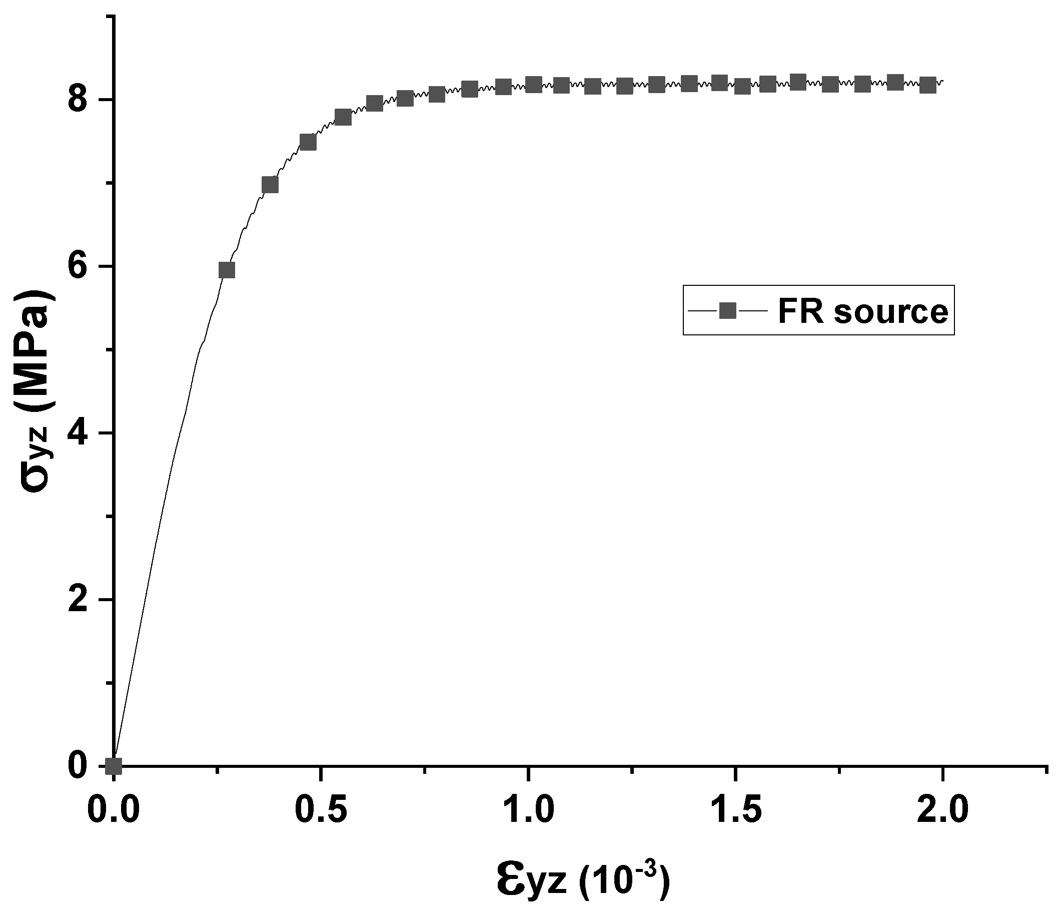
Figure 4.
(a,c,e) (dark blue) A spiral dislocation source with one end fixed at the origin of the coordinate system by a pinning point while the other end is free; (b,d,f) (red) a spiral dislocation source with one end fixed at the origin of the coordinate system by an extended dislocation while the other end is free (simulation box dimensions: S1 = S2 = S3 = 600,000b). Figures (a,b) are the initial configurations. Figures (c,d) show the initial bowing of the source. Figures (e,f) show multiple loops of the dislocation source.
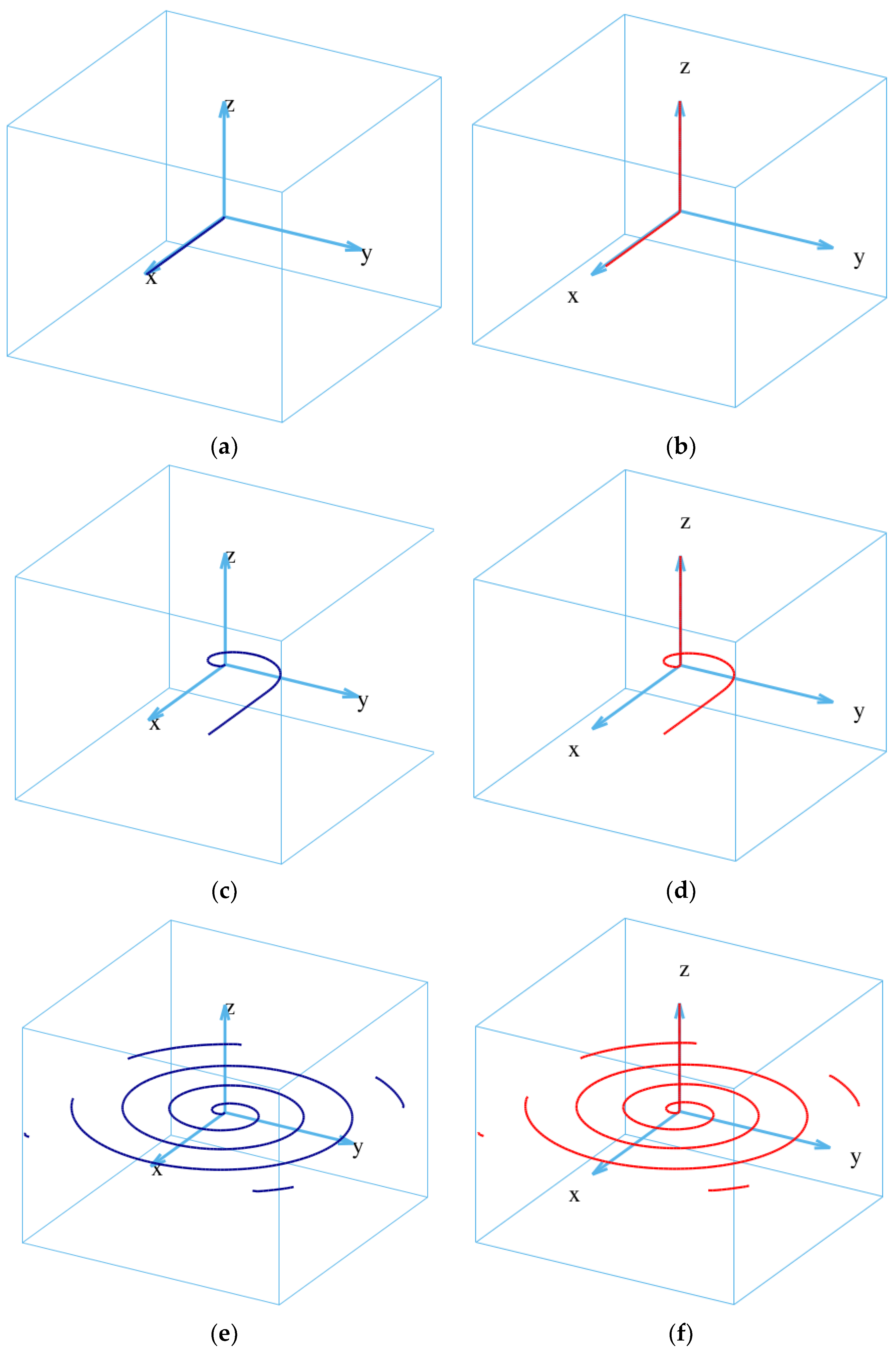
Figure 5.
Stress–strain diagram for DDD simulations using various S2 values (other simulation box dimensions: S1 = S3 = 60,000b). Here, no surface effect is accounted for.
Figure 5.
Stress–strain diagram for DDD simulations using various S2 values (other simulation box dimensions: S1 = S3 = 60,000b). Here, no surface effect is accounted for.
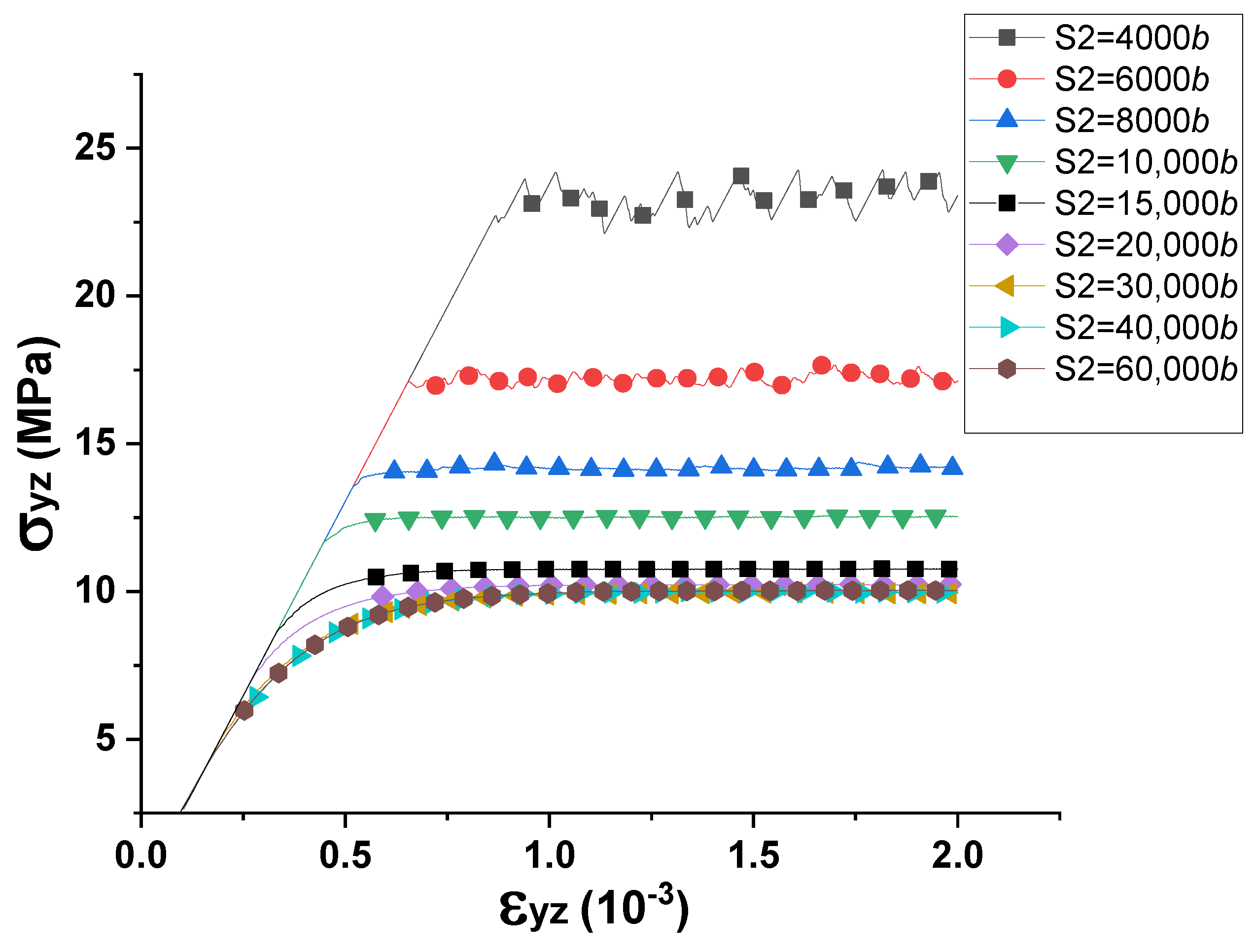
Figure 6.
Flow stress (mean values of the steady-state portions of the Stress–strain curves in Figure 5) vs. S2 (without surface effect).
Figure 6.
Flow stress (mean values of the steady-state portions of the Stress–strain curves in Figure 5) vs. S2 (without surface effect).

Figure 7.
(a) A spiral dislocation source in a simulation box with dimensions S1 = S2 = 60,000b and S3 = 40,000b; (b) a spiral dislocation source in a simulation box with dimensions S1 = 60,000b, S3 = 40,000b, and S2 = 6000b (without surface effect).
Figure 7.
(a) A spiral dislocation source in a simulation box with dimensions S1 = S2 = 60,000b and S3 = 40,000b; (b) a spiral dislocation source in a simulation box with dimensions S1 = 60,000b, S3 = 40,000b, and S2 = 6000b (without surface effect).
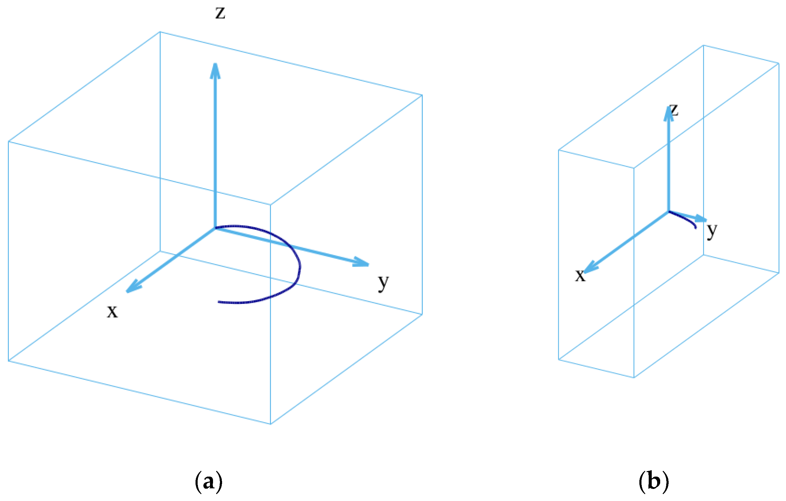
Figure 8.
DDD simulation for two spiral dislocations (red lines in the figures) initially with edge character at different time steps (without surface effect).(a) Initial configuration of two edge spiral dislocations; (b) Operation of the edge spiral dislocations under a constant shear strain rate; (c) Formation of traditional screw FR source; (d–f) Operation of the traditional screw FR source under a constant shear strain rate.
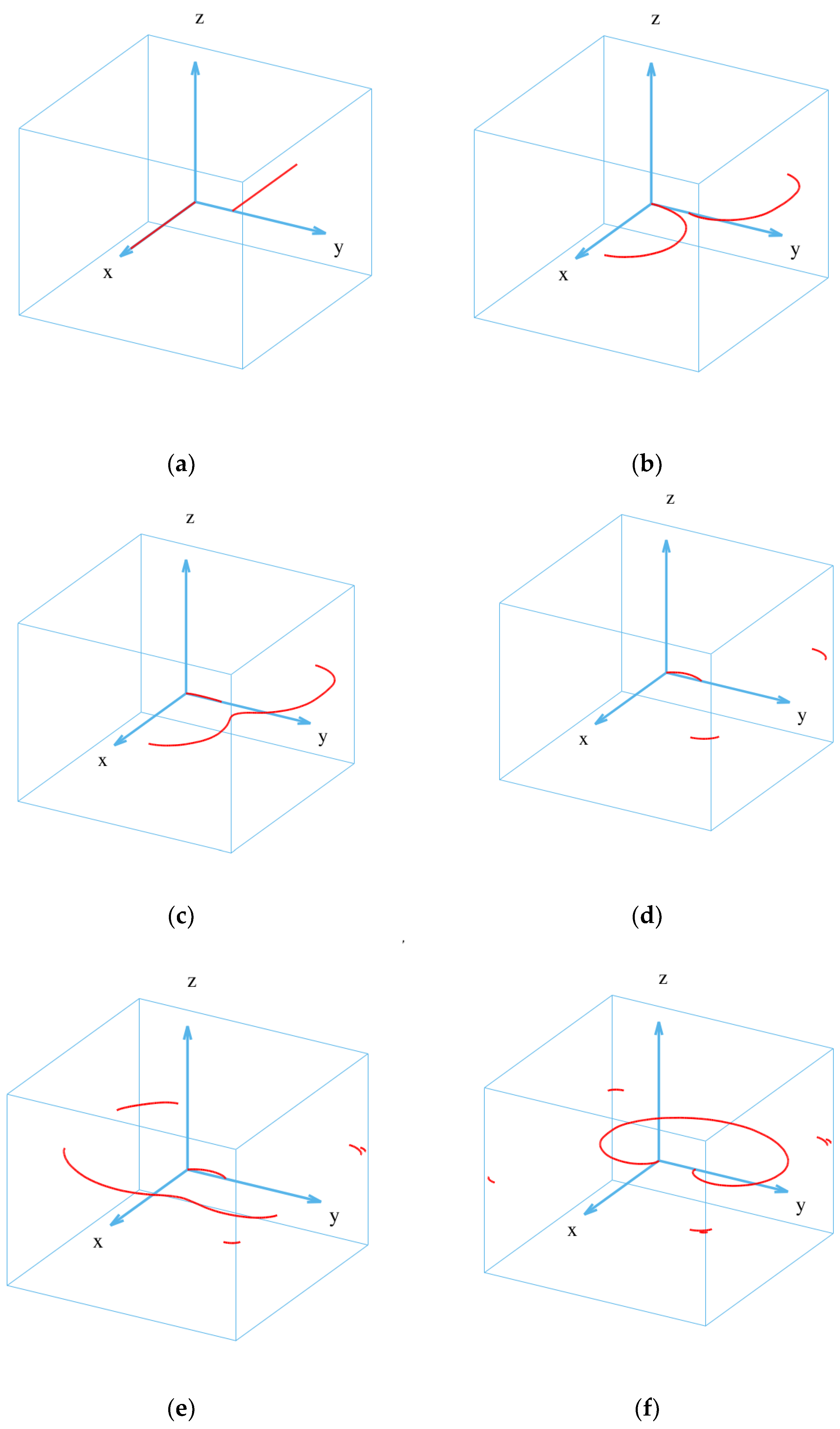
Figure 9.
DDD simulation for two spiral dislocations initially with screw character at different time steps (without surface effect). (a) Initial configuration of two screw spiral dislocations; (b) Operation of the screw spiral dislocations under a constant shear strain rate; (c) Formation of traditional edge FR source; (d–f) Operation of the traditional edge FR source under a constant shear strain rate.

Figure 10.
Simulation data for two edge spiral dislocations and a Frank–Read screw dislocation source (Simulation box dimensions: S1 = S2 = 60,000b and S3 = 40,000b (without surface effect)).
Figure 10.
Simulation data for two edge spiral dislocations and a Frank–Read screw dislocation source (Simulation box dimensions: S1 = S2 = 60,000b and S3 = 40,000b (without surface effect)).
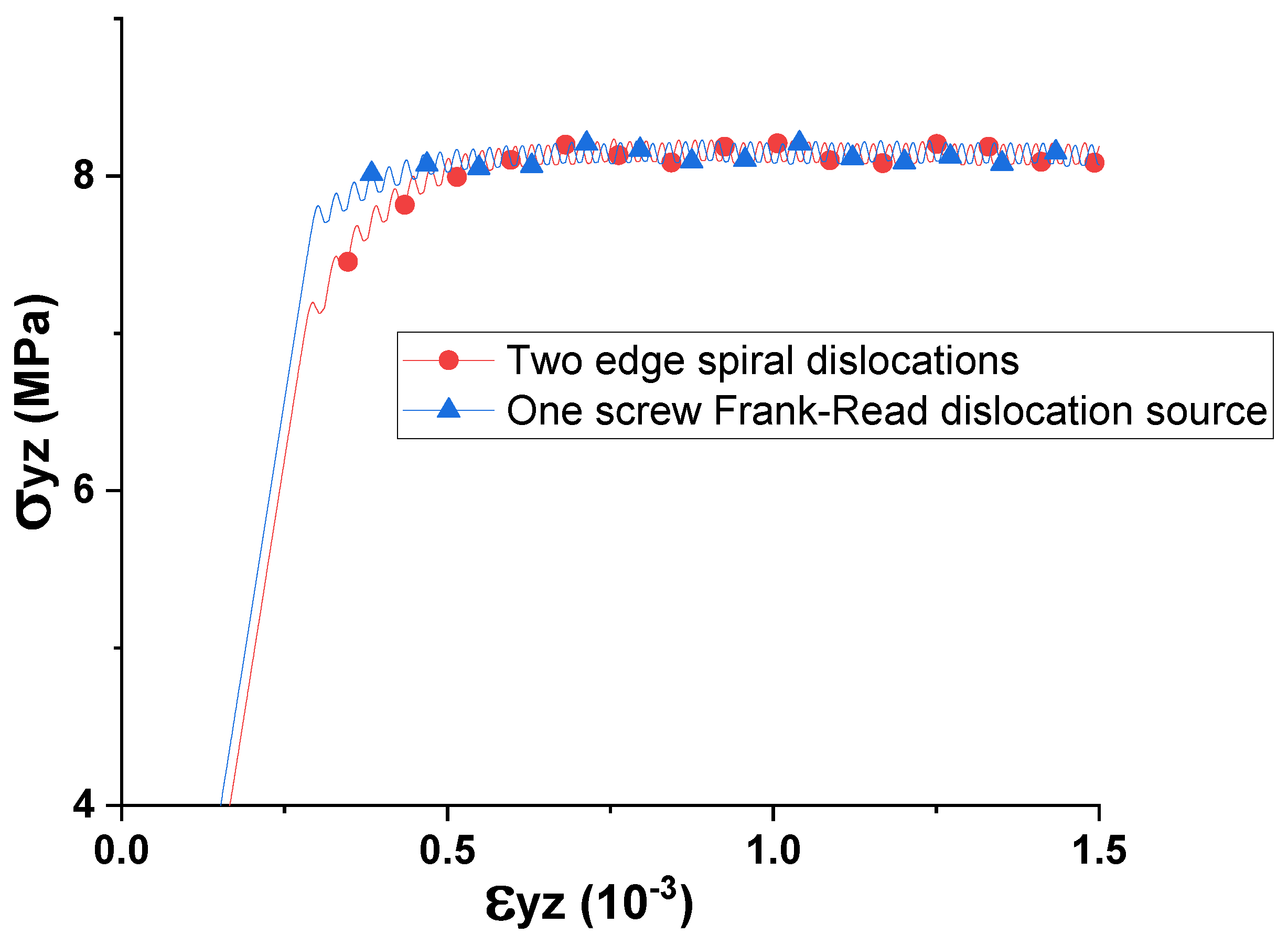
Figure 11.
Spiral dislocation source multipoles of edge character, with constant separation 1000b along the z-axis. (a) Dipole, (b) tripole, and (c) quadrupole (no surface effect).
Figure 11.
Spiral dislocation source multipoles of edge character, with constant separation 1000b along the z-axis. (a) Dipole, (b) tripole, and (c) quadrupole (no surface effect).
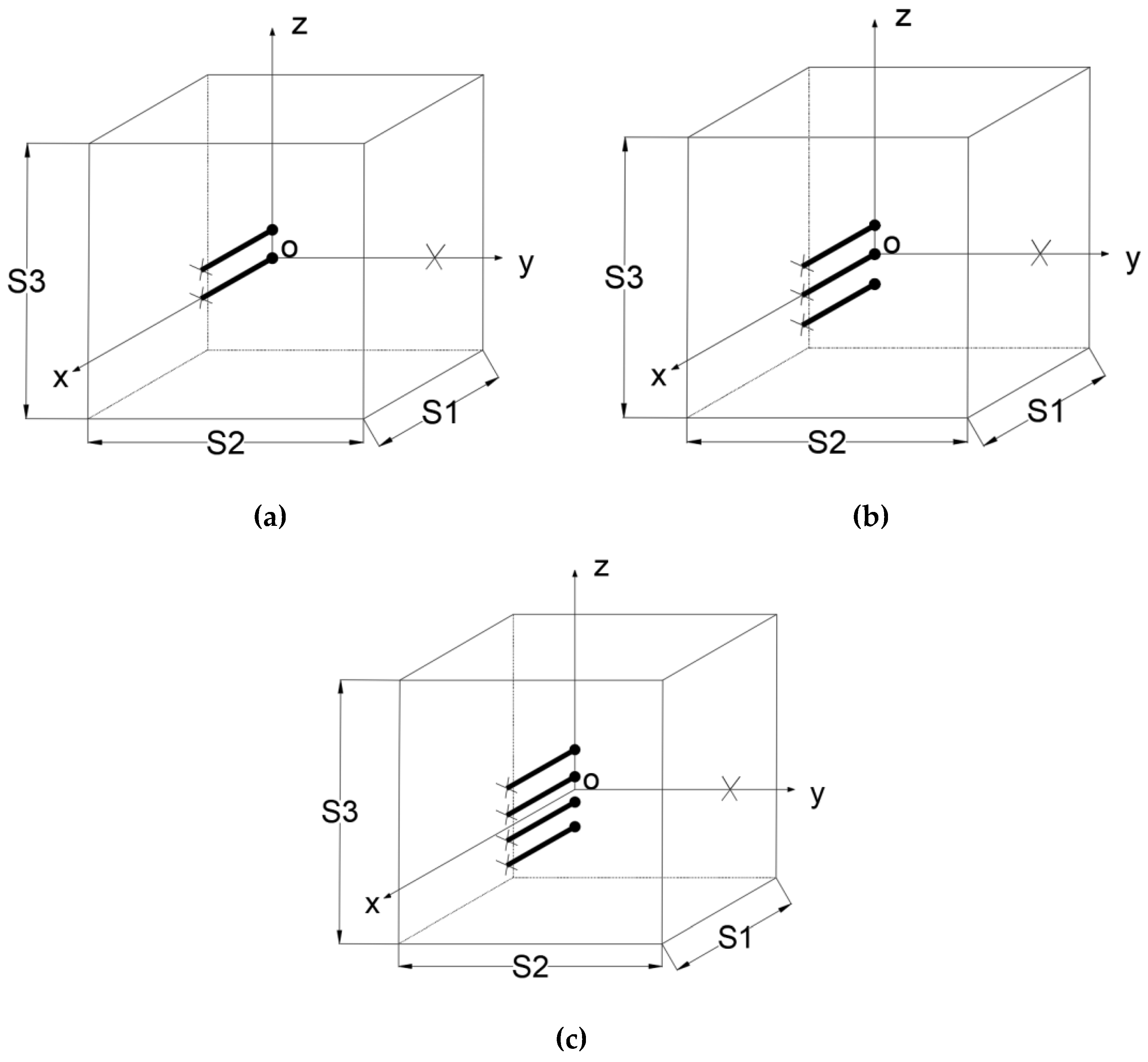
Figure 12.
Single and multipoles (see Figure 11) in action. They act as a fan with multiple blades. (a) Single, (b) dipole, (c) tripole, and (d) quadrupole (no surface effect). (Different color lines in the figures represent the spiral dislocation sources separated along the z-axis.)
Figure 12.
Single and multipoles (see Figure 11) in action. They act as a fan with multiple blades. (a) Single, (b) dipole, (c) tripole, and (d) quadrupole (no surface effect). (Different color lines in the figures represent the spiral dislocation sources separated along the z-axis.)


Figure 13.
(a) Stress–strain curves for multipoles simulations. (b) Flow stress vs. the number of spiral sources of the multipoles.
Figure 13.
(a) Stress–strain curves for multipoles simulations. (b) Flow stress vs. the number of spiral sources of the multipoles.
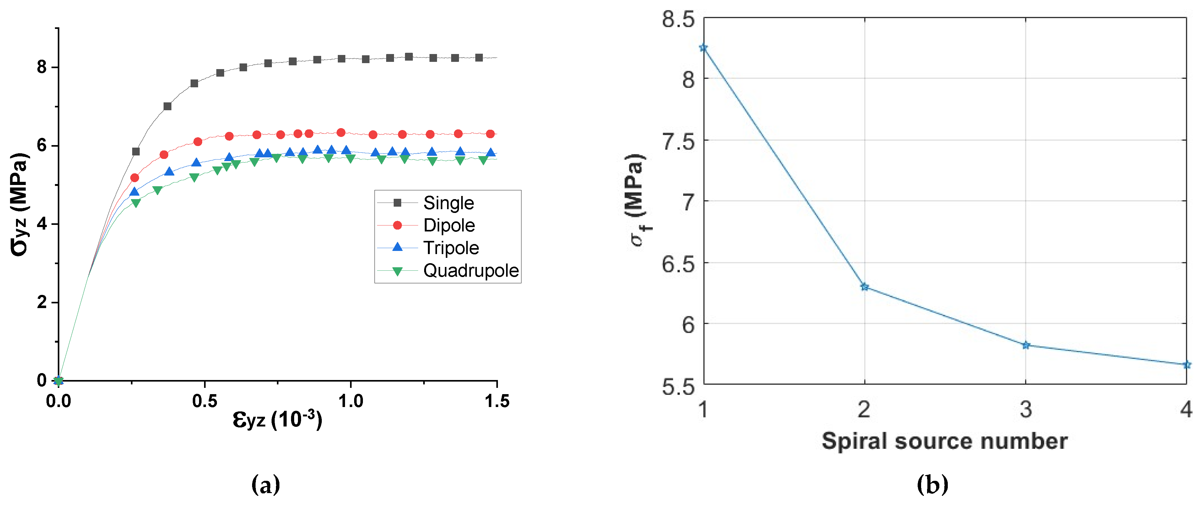
Figure 14.
The DDD simulation for a spiral dislocation (purple line in the figures) near a free surface with surface effect activated (Top view). (a) Initial configuration of the simulation; (b,c) The spiral dislocation is attracted towards the free surface under the effect of the image stress and almost touches the surface in (c); (d) The spiral dislocation eventually vanishes at the free surface with its two ends still in the crystal.

Disclaimer/Publisher’s Note: The statements, opinions and data contained in all publications are solely those of the individual author(s) and contributor(s) and not of MDPI and/or the editor(s). MDPI and/or the editor(s) disclaim responsibility for any injury to people or property resulting from any ideas, methods, instructions or products referred to in the content. |
© 2023 by the authors. Licensee MDPI, Basel, Switzerland. This article is an open access article distributed under the terms and conditions of the Creative Commons Attribution (CC BY) license (https://creativecommons.org/licenses/by/4.0/).
Share and Cite
MDPI and ACS Style
Li, L.; Khraishi, T. An Investigation of Spiral Dislocation Sources Using Discrete Dislocation Dynamics (DDD) Simulations. Metals 2023, 13, 1408. https://doi.org/10.3390/met13081408
AMA Style
Li L, Khraishi T. An Investigation of Spiral Dislocation Sources Using Discrete Dislocation Dynamics (DDD) Simulations. Metals. 2023; 13(8):1408. https://doi.org/10.3390/met13081408
Chicago/Turabian StyleLi, Luo, and Tariq Khraishi. 2023. "An Investigation of Spiral Dislocation Sources Using Discrete Dislocation Dynamics (DDD) Simulations" Metals 13, no. 8: 1408. https://doi.org/10.3390/met13081408
Note that from the first issue of 2016, this journal uses article numbers instead of page numbers. See further details here.