Article

Algorithms to Estimate the Ductile to Brittle Transition Temperature, Upper Shelf Energy, and Their Uncertainties for Steel Using Charpy V-Notch Shear Area and Absorbed Energy Data

1
Engineering Department, American University of Iraq, Sulaimani 46001, Iraq
2
RSI-Pipeline Solutions, New Albany, OH 43054, USA
3
Pacific Gas and Electric Company, Walnut Creek, CA 94598, USA
*
Author to whom correspondence should be addressed.
Metals 2023, 13(5), 877; https://doi.org/10.3390/met13050877
Submission received: 10 February 2023 / Revised: 24 April 2023 / Accepted: 25 April 2023 / Published: 2 May 2023
(This article belongs to the Special Issue Computer Methods in Metallic Materials (Volume II))

Abstract

:
Toughness and the transition from ductile to brittle behavior are long-standing concerns for applications of ferritic steel such as line-pipe. Three algorithms have been developed to fit a hyperbolic tangent curve to any Charpy V-notch dataset and estimate the uncertainty for (1) the 85% shear appearance area transition temperature and (2) the upper shelf absorbed energy. To fit the hyperbolic tangent curve to the data the (I) first algorithm relied on iterative estimation of four-parameters; (II) the second algorithm on two parameters (after simplification based on physical assumptions); and (III) the third algorithm on only one parameter (after further simplification). The algorithms were written using the open-source programing language, R. The minimum input requirements for the algorithm are experimental data for shear appearance area and absorbed energy from at least four temperatures for the four-parameter algorithm, two temperatures for the two-parameter algorithm, and one temperature for the one-parameter algorithm. The test temperatures and quantity of tests at each temperature can vary. The algorithms are described in detail and demonstrated using a data set of 12 Charpy test results (shear area and absorbed energy) from one API-5L grade X52 pipe with 4.5 mm thick Charpy bars. A future paper will test and compare the algorithms using a wide variety of Charpy V-notch data sets to clarify their applicability and possible limitations.

Graphical Abstract

1. Introduction

1.1. Importance of Toughness Testing

Toughness can be viewed as a measure of the amount of energy required to cause a rapid fracture. In the 1800s and early 1900s, brittle, low-toughness iron and steel caused many catastrophic failures [1,2,3,4,5]. Specifically, for steel pressure vessels and pipes, toughness has been recognized as a critical parameter for evaluating burst pressure for over 100 years [6]. In the early 1900s, various impact tests were developed, originally to test the quality of armor plate and boiler steels, and the ASTM E23 method for Charpy impact testing procedure was tentatively released in 1933 [1]. The use of Charpy testing has expanded greatly, and examples of industries that rely on Charpy testing today include shipbuilding [7,8,9], nuclear power [10,11], armor [12], rail [13,14], construction [15], steam turbine [16], piping and pressure vessel [17,18,19], liquified natural gas storage [20], hydrogen storage [21], additive manufacturing [22], aluminum alloy development [23], and composites [24]. The principles and methods described in this paper are relevant to many critical structural applications but will be analyzed and discussed with respect to steel line pipes widely used in natural gas and hazardous liquid pipelines.

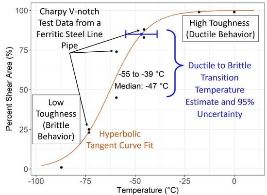
1.2. Charpy Testing to Assess Steel Ductile and Brittle Behavior

Toughness is often evaluated using a Charpy test. The standard sample for a Charpy test exhibits a 10 mm by 10 mm cross-section and a 2 mm notch. The sample is dynamically fractured using a gravity-driven hammer. The energy lost by the hammer is recorded and equated to the energy absorbed by the sample. The shear appearance area is measured from the fracture surface of the sample. The absorbed energy and shear appearance correlate to the toughness behavior of the steel.
Ferritic steels typically exhibit a transition from ductile behavior (high energy absorption) at room temperature to brittle behavior at low temperatures [25]. Structural steel alloys, including those used for line pipe, are intended for use in their ductile regime. Often, pipeline operators desire to know the ductile to brittle transition temperature to establish a safe operating temperature range within which the material is likely to behave in a ductile manner, thereby reducing the risk of catastrophic brittle failure.
When manufacturing line pipe, Charpy tests are usually required to be performed for only one or two temperatures. ASME Boiler and Pressure Vessel Code Section XI (Division 1, Paragraph IWA-4665), API 5L, and ASTM A370 require a minimum toughness based on three tests at one temperature. These tests enable pipe manufacturers and pipeline operators to ensure sufficient toughness relative to some intended operating temperature. However, Charpy testing at a single temperature is insufficient to quantify the change in absorbed energy and shear appearance relative to temperature. Charpy test results from multiple temperatures are necessary to enable the characterization of the transition from ductile behavior to brittle behavior. Thus, operators sometimes request “full Charpy curves”, i.e., Charpy tests performed at multiple temperatures (8–12) to characterize the transition from ductile to brittle behavior and upper shelf energy.

1.3. Methods to Estimate Upper Shelf Absorbed Energy

Absorbed energy, E , versus test temperature, T t e s t . Absorbed energy, E , forms a sigmoidal curve when plotted versus test temperature, T t e s t . Oldfield (1975) recognized that the most appropriate function for fitting Charpy data is the hyperbolic tangent [26]:
E = A E + B E tanh T t e s t D E C E .
A E are B E are defined as:
A E = E U S + E L S 2 ,   a n d
B E = E U S E L S 2
where E U S is the upper shelf absorbed energy and E L S is the lower shelf absorbed energy. The constant, C E , is the halfwidth of the transition region such that the slope of the transition region is equal to B E / C E . The constant, D E , is the midpoint of the hyperbolic tangent function. The relationships between the constants, A E , B E , C E , and D E , are demonstrated by Figure 1.

1.4. Methods to Estimate Ductile to Brittle Transition Temperature

Along with the E U S it is common to characterize the toughness of a type of steel using the transition temperature [27]. Owing to the transition being generally continuous, there are various definitions for transition temperatures in different industries such as the 28 J transition temperature from BS 7910 [28,29], the 47 J transition temperature for the nuclear industry [30], and the 50% cleavage transition temperature ( T 50 ) used in the shipbuilding industry [9]. In the pipeline industry, the 85% shear appearance area transition temperature ( T 85 ) is referenced for two reasons. Firstly, shear appearance is considered a better indicator of transition behavior than absorbed energy for metals with different processing histories [9]. Secondly, fully ductile behavior can be assumed to be predominant for temperatures above the T 85 [31,32]. Note that the Charpy test is a dynamic test and usually results in a ductile to brittle transition temperature that is much higher than the ductile to brittle transition temperature for crack initiation, which is more relevant for steel line pipe failures [31]. However, it is an important measure of the ability of a pipeline material to arrest a propagating fracture. The test also lends itself to evaluating product specification conformity during manufacturing.

1.5. Methods to Estimate Uncertainty

The T 85 and E U S are useful for fitness-for-service and risk assessments, maximum flaw size estimation, maintenance and replacement procedure development, and ground shift risk mitigation [31]. The T 85 and E U S are usually estimated by manually drawing or plotting a sigmoidal, hyperbolic tangent curve through the data (e.g., Refs. [28,33]). This labor-intensive, qualitative method requires curves to be evaluated one-by-one and does not provide a quantitative estimate of uncertainty. Oldfield developed a least squares curve fitting method, but the method does not provide an estimate for uncertainty, could be difficult to apply, and, for some data sets, may not converge in a satisfactory manner [26]. Lucon et al. presented an algorithm to fit the hyperbolic tangent function, but the algorithm requires having multiple tests exhibiting > 95% shear appearance area and multiple tests exhibiting < 5% shear appearance area [34]. Orynyak et al. developed an analytical method for calculating transition temperature uncertainty, but the method can be difficult to implement [30]. Marini described a Monte Carlo method to estimate probability distributions of the transition temperature and upper shelf energy, but it requires manual adjustment of the probability distributions for the input parameters [29]. Recently, Anderson et al. published the concept of a four-parameter (general) algorithm and two-parameter (simplified) algorithm for predicting the T 85 and E U S and their uncertainty [35]. The current study presents these algorithms in detail, and discusses their advantages, and disadvantages, and adds a one-parameter algorithm to the discussion and comparison.

1.6. Objectives and Research Significance

The main aim of the present work was to develop new algorithms that can estimate T 85 and E U S for several CVN datasets. It is important that the algorithms be robust (converge for data with varying numbers of test temperatures, different spacings between the test temperatures, and varying amounts of uncertainty). An understanding of uncertainty is critical for risk assessments and fitness for service decisions in the pipeline industry, and there is currently no standard method or algorithm to estimate uncertainty in predictions of shear appearance transition temperature and upper shelf energy. Therefore, the proposed algorithms should provide a consistent method for estimating that uncertainty.

1.7. Outline

This article will provide a detailed presentation of the three algorithms that were developed based on the hyperbolic tangent model from API 579 Fitness for Service Annex 9F Material Properties for Crack-like Flaws Section 2.3 Charpy V-notch Transition Curve [32]. The proposed algorithms include: (1) a four-parameter algorithm requiring the input of shear appearance area and absorbed energy data for at least four different temperatures, (2) a two-parameter algorithm requiring the same data from only two different temperatures, and (3) a one-parameter algorithm requiring the same data from a minimum of only one temperature. An open-source statistical programing language, R (version 4.1.1 10 August 2021) was used for algorithm development. The algorithms are herein described in detail.
The algorithms are demonstrated using a data set of 12 Charpy test results (shear area and absorbed energy) from one API-5L grade X52 pipe with 4.5 mm thick Charpy bars. A future paper will test and compare the algorithms using a large data set to identify the limitations of the algorithms. The predictions of shear appearance transition temperature and upper shelf energy and uncertainty for each algorithm are compared and discussed in terms of the effects of the algorithm assumptions and constraints. The advantages and disadvantages of each algorithm are discussed along with approaches to planning Charpy test temperatures such that the data will result in reliable predictions of T 85 and E U S .

2. Materials and Methods

2.1. Material

The steel pipe from which the Charpy test samples were machined was an API-5L grade X52 electric resistance welded pipe manufactured in ~1972. The Charpy test bars were machined from base metal (not the weld). The pipe had an outside diameter of 324 mm and a reported nominal wall thickness of 5.56 mm. The steel pipe composition was tested using optical emission spectroscopy and is given in Table 1.

2.2. Charpy Bar Machining and Testing

The 12 Charpy test bars were oriented in the longitudinal direction (the length of the Charpy bar aligned with the rolling direction of the original plate) such that the crack grew in the transverse direction (perpendicular to the rolling direction). The sample thickness was 4.5 mm. Two tests at each the of six temperatures were conducted using a standard Charpy hammer that recorded the absorbed energy. The guidance on how to interpret shear appearance area and absorbed energy for Charpy samples from ASTM E23 [25] was followed and the results are shown in Table 2. The assumed amount of error for these data points is discussed in the section entitled “Monte-Carlo simulation for error and uncertainty estimation”.

2.3. Algorithm Overview

Three algorithms were written to estimate the 85% shear appearance transition temperature ( T 85 ) and the upper shelf absorbed energy ( E U S ) for Charpy V-notch data sets. The purpose of the algorithms was to fit the hyperbolic tangent function to the data. The fitting was first attempted using the nonlinear least squares fitting function, “nls”, available in the R package, “stats”. In preparation for the algorithms, the nls function was tested for its applicability to a large database with a wide variety of Charpy V-notch data sets, but the nls function was unable to converge for some data sets. Therefore a novel non-linear least squares fitting function based on the Levenberg–Marquardt method [36,37], “nlsLM” available in the R package, “minpack.lm” [38,39] was used. The complete R-Markdown code for all three algorithms is contained in Appendix A, and the theoretical bases for the code will be described here.

2.3.1. Shear Appearance Area vs. Test Temperature

All three algorithms first fit the hyperbolic tangent function to the shear appearance area vs. temperature data. Shear appearance area, S , forms a sigmoidal, hyperbolic tangent curve when plotted versus test temperature, T t e s t [31]:
S = A S + B S tanh T t e s t D S C S .
The constants A S and B S are defined based on API 579 equation 9F-14 and 9F-15 as follows [32]:
A S = S U S + S L S 2   a n d
B S = S U S S L S 2 ,
where S U S is the upper shelf for the shear appearance area, and S L S is the lower shelf for the shear appearance area. Thus, the parameter A S defines the vertical center point of the hyperbolic tangent curve and B S defines the vertical half-width. Similarly, D S defines the horizontal center point of the hyperbolic tangent curve and C S defines the horizontal half-width.

2.3.2. Absorbed Energy vs. Test Temperature

All three algorithms then fit the hyperbolic tangent function to the absorbed energy vs. temperature data. Similar to shear appearance area, absorbed energy, E , forms a sigmoidal, hyperbolic tangent curve when plotted versus test temperature, T t e s t [32], as shown by Equation (1):
E = A E + B E tanh T t e s t D E C E .
where A E are B E were defined by Equations (2) and (3) as:
A E = E U S + E L S 2 ,   a n d
B E = E U S E L S 2 .
where E U S and E L S are the upper and lower shelf, respectively, for the absorbed energy. Again, the parameter A E defines the vertical midpoint of the hyperbolic tangent curve and B E defines the vertical half-height. Similarly, D E defines the horizontal midpoint of the hyperbolic tangent curve and C E defines the horizontal half-width.

2.4. Four-Parameter Algorithm

The first algorithm used to find a solution was a four-parameter algorithm wherein none of the hyperbolic function’s constants were initially defined.

2.4.1. Calculation of Parameters A S , B S , C S , and D S and T 85

The algorithm begins with the initial values for the constants as follows: A S , i = 50 % and B S , i = 50 % . D S , i is taken as the test temperature where the shear area is closest to 50%; and C S , i is calculated as half of the interquartile range for the test temperatures. Since the model is fit based on whole numbers for percentages rather than decimal equivalent the shear area, A S , i , is fixed at 50 rather than 0.5. If decimal equivalents to percentage are used to fit the model 0.5 would be used in the equation.
To estimate T 85 , first, the nlsLM function iteratively calculates the values of the four constants, A S , B S , C S , and D S to find the values that minimize the mean square error between the observed and predicted values. The max number of iterations was fixed at 100 for all runs. To identify the shear area transition temperature, T 85 , the shear area data for each individual data set were fit to the hyperbolic tangent curve. The T 85 is calculated by rearranging Equation (4) to calculate the inverse hyperbolic tangent as follows:
T 85 = tanh 1 S A S B S × C S + D S .
where a shear area, S , value of 85% was input in the formula to evaluate the function per the definition of T 85 .

2.4.2. Calculation of Parameters A E , B E , C E , and D E and E U S

The algorithm calculates the initial values for the constants as follows:
A E , i = E m a x + E m i n 2   a n d
B E , i = E m a x E m i n 2
where E m a x and E m i n are the largest and smallest absorbed energy readings in the data set, respectively. The test temperature where the shear area was closest to 50% is taken as D E , i ; and C E , i is calculated as half of the interquartile range for the test temperatures.
The four-parameter algorithm uses the nlsLM function to converge on a solution for the constants, A E , B E , C E , and D E , with no constraints. The constants D E and C E should be numerically close to D S and C S since these constants relate to the center and width of the transition zone in terms of the horizontal axis variable, temperature. The model calculates E U S by rearranging Equations (2) and (3) as follows:
E U S = A E + B E .

2.5. Two-Parameter Algorithm

The second algorithm was a two-parameter algorithm that sought to improve the chances of convergence by defining A S , B S , C E , and D E based on physical principles. Since the focus of the effort was to apply these automated algorithms to a large database of Charpy V-notch data sets, the two-parameter algorithm was developed with the intent of enabling the fit to converge for more Charpy data sets in case, for example, a few Charpy samples could be extracted and tested from the pipe or test temperatures were poorly chosen and led to narrow ranges of resulting shear appearance area and absorbed energy values.
Assuming the shear appearance area for the upper shelf is 100% and the shear appearance lower shelf is 0%, then the fitting terms, A S , and B S become
A S = S U S + S L S 2 = 100 % + 0 % 2 = 50 % a n d
B S = S U S S L S 2 = 100 % 0 % 2 = 50 % .
Thus, the nlsLM function is left only to solve for two parameters, D S and C S as shown:
S = 50 % + 50 % tanh T t e s t D S C S .
Then, the 85% shear appearance transition temperature is calculated as
T 85 = tanh 1 85 % 50 % 50 % × C S + D S 0.867 × C S + D S .
Next, understanding that C S , represents the halfwidth of the transition region and D S represents the midpoint of the hyperbolic tangent curve, these values should be the same as C E and D E , respectively, for absorbed energy vs. temperature. Therefore, the two-parameter algorithm equates these parameters (i.e., D S = D E and C S = C E ):
E = A E + B E tanh T t e s t D S C S .
The nlsLM function is left only to solve for two parameters, A E and B E . Then the upper shelf energy is calculated using Equation (10).
For the two-parameter algorithm the nlsLM function iterates on the four constants, C S , D S , A E , and B E to converge to a solution compared with eight for the four-parameter algorithm. This reduction of unknowns increases the probability of finding a solution and allows a reduction of the minimum number of required data points. The minimum input data requirement for the two-parameter algorithm is the shear appearance area and absorbed energy data from at least two different temperatures (at least one test per temperature).

2.6. One-Parameter Algorithm

The third algorithm is a further simplification from API 579 that defined most of the parameters and only left D S and A E for the calculation. The one-parameter algorithm was first published by Rosenfeld [31], and later included in API 579 [32] and gives the relationship between shear appearance area and test temperature as:
S = 1 + exp T t e s t T 85 + C A C B 1 ,
where T t e s t is the test temperature and C A and C B are known as the sigmoidal parameters from API 579, listed in Table 3. Equation (16) is equivalent to:
S = 1 2 1 + t a n h T t e s t T 85 + C A 2 C B .
The sigmoidal parameters depend on sample thickness and were empirically derived from tests on a variety of pipeline steels. They are sets of temperature offsets that help describe the width of the transition region. For ease of interpolation for non-standard Charpy sample thicknesses we fit these sigmoidal parameters to the following equations where t is the Charpy sample thickness in mm:
C A = 11.1 × ln t + 2.1 ,   a n d
C B = 5.7 × ln t + 6.3 .
The empirically determined sigmoidal parameters, C A and C B , relate to the hyperbolic tangent parameters from the simplified model as D S = T 85 C A and C S = 2 C B . Thus, Equation (17) is equivalent to:
S = 50 % + 50 % tanh T t e s t D S C S
For example, for a full size (10 mm) Charpy V-notch sample, the sigmoidal parameter C B = 18 ° C defines the half-width of the transition region, C S , as 36 °C. Therefore:
T 85 = tanh 1 85 % 50 % 50 % × C S + D S 0.867 × 2 C B + D S
Thus, the only fitting parameter for which to solve for the one-parameter model for shear area is D S , the midpoint of the hyperbolic tangent curve.
Next, the one-parameter algorithm states that each sample’s absorbed energy is proportional to 90% of the sample shear area plus a 10% offset:
E U S = E t e s t 0.9 × S t e s t + 0.1
where E t e s t and S t e s t are the sample absorbed energy and shear appearance area measurements, respectively. The underlying assumption therefore is that the lower shelf energy is 10% of the upper shelf energy. Substituting these values into Equations (2) and (3), we obtain:
A E = E U S + 0.1 E U S 2 ,   a n d
B E = E U S 0.1 E U S 2 .
Solving the above system of equations leads to B E = 0.818 A E , and plugging this relationship into Equation (15) gives:
E = A E 1 + 0.818 tanh T t e s t D S C S .
The 10% offset ensures that the predicted lower shelf of the absorbed energy matches the physical reality that absorbed energy is always above zero. The C S is again calculated from the sigmoidal parameter as C S = 2 C B , and the D S value is carried over from the shear area curve fit. The upper shelf energy becomes:
E U S = 1.818 A E .
In summary, the one-parameter algorithm is like the two-parameter algorithm except with the two additional assumptions that (1) the width of the transition zone is known, and (2) that the absorbed energy lower shelf is 10% of the upper shelf. These additional assumptions allow the algorithm to find a solution with only one data point, i.e., values for shear area and absorbed energy for one temperature.

2.7. Monte-Carlo Simulation for Error and Uncertainty Estimation

In any regression solution, the assumption is that all the residual error between the model and the observations follows a distribution with a mean of zero and a common variance across the entire range of the independent variable. This is not likely the case as there is a physical limitation of the shear area being between 0 and 100%, and the absorbed energy being greater than zero, therefore the potential absolute error at lower temperatures is going to be much smaller than at higher temperatures.
To account for the uneven variance in shear estimates and absorbed energy, and their effect on the model solution, a Monte Carlo (MC) simulation was employed. In the MC process, the shear area and absorbed energy are treated as normally distributed stochastic variables with a mean equal to the observed value. For the shear area, the standard deviation was assumed to be 5% of the observed value based on ASTM E23. For absorbed energy, the standard deviation was assumed to be a minimum of 0.6 J and increase with increasing absorbed energy measurement, as prescribed by ASTM E23 at a rate of 2.6% of the value (i.e., a b s o r b e d   e n e r g y   s t a n d a r d   d e v i a t i o n = 0.6 + 0.026 × m e a s u r e d   v a l u e ).
For each temperature, 1000 pairs of the test temperatures and absorbed energy or shear areas are generated. After the data is generated, a solution is created for each set of data, and the 95% sample quantile for each of the coefficients is calculated. The benefit of using the sample quantile is that it makes no assumption about the distribution of the coefficient solutions such as following a normal or t-distribution. It uses the quantiles from the empirical distribution of results, thus preserving any skew to the data. In this study, the median value and 95% quantile (uncertainty) are used for comparison with the parameter estimates and confidence intervals between the three algorithms.

3. Results

First, for the example shear appearance area vs. temperature data from Table 2, all three algorithms were used to fit the hyperbolic tangent curve and generate the values for the parameters, A S , B S , C S , and D S , and their associated standard error ( ϵ ) as given in Table 4. The four-parameter algorithm iteratively adjusted all four parameters to fit a hyperbolic tangent curve to the data. On the contrary, for the two-parameter and one-parameter the A S and B S parameters were set to 50 so that the hyperbolic tangent fitting curve for shear appearance area must stay within the limitations of 0–100%. Furthermore, for the one-parameter algorithm the C S was calculated to be 29.7 based on inserting the sample thickness, 4.5 mm, into Equation (19) to calculate C B and finding C S using the relationship, C S = 2 C B . The relative agreement between all the parameters in each column is represented by the similar shapes of the hyperbolic tangent curves in Figure 2, Figure 3 and Figure 4.
Second, for the example absorbed energy vs. temperature data from Table 2, all three algorithms were used to fit the hyperbolic tangent curves and generate the values for the parameters, A E , B E , C E , and D E , and their associated standard error ( ϵ ) as given in Table 5. The four-parameter algorithm iteratively adjusted all four parameters to fit a hyperbolic tangent curve to the data. On the contrary, for the two-parameter and one-parameter the C E and D E parameters were assumed to equal C S and D S . For the one-parameter algorithm the B E was set to 0.818 A E based on Equation (26). The relative agreement between all the parameters in each column is represented by the similar shapes of the hyperbolic tangent curves in Figure 5, Figure 6 and Figure 7.

3.1. Estimates of Shear Appearance Transition Temperature ( T 85 )

Firstly, we will compare the three algorithms in terms of their estimation of T 85 . For the four-parameter algorithm, the Charpy V-notch shear area versus temperature data (black points), the hyperbolic tangent fit (orange line), and the 95% quantile for T 85 are shown in Figure 2. The estimate for T 85 (median) is shown as −46 °C, and the 95% quantile is shown as −66 to −26 °C. One issue with the four-parameter algorithm is that the lower shelf (lower left) goes below zero, which is physically impossible. There cannot be a shear appearance area measurement below 0% shear appearance area.
For the two-parameter algorithm the hyperbolic tangent fit is shown in Figure 3. The two-parameter model fixed the lower shelf shear appearance area at 0% to avoid the physical impossibility of a negative shear appearance area and fixed the upper shelf shear appearance area at 100% to avoid the physically impossible shear appearance area > 100%. The T 85 median value is −47 °C, nearly the same as for the four-parameter model. The error range for the two-parameter model, −55 to −39 °C, is much smaller than that for the four-parameter model because there were fewer parameters.
For the one-parameter algorithm, the hyperbolic tangent fit is shown in Figure 4. The lower and upper shelf shear appearance area were fixed at 0% and 100%, respectively, like the two-parameter. Additionally, the one-parameter model assumed the half-width of the transition region ( C S ) as two times the sigmoidal parameter B ( C B ) , thus C S = 2 C B . C B was calculated using Equation (19). One issue is that the calculated C S parameter appears to be larger than what would be expected from the data. Observe from Table 4 that the C S value for the four-parameter and two-parameter models was 18–19 °C, whereas the assumed C S for the one-parameter model is nearly 30 °C. Mostly due to the excessive C S estimate, the median estimate for T 85 , −36 °C, was higher than that for the four-parameter and two-parameter models. The range, −42 to −31 °C was the smallest because only one parameter contributed error and the other three were fixed with an effective uncertainty of zero. But observe that the one-parameter algorithm exhibits the largest differences between the observed and predicted values represented by the curve.

3.2. Estimates of Upper Shelf Energy ( E U S )

Secondly, we will compare the three algorithms in terms of their estimation of E U S . For the four-parameter algorithm, the Charpy V-notch absorbed energy versus temperature data (black points), the hyperbolic tangent fit (orange line), and the 95% quantile for E U S are shown in Figure 5. The estimate for E U S is shown as 46 ± 8 J. For the two-parameter algorithm is shown in Figure 6, showing an estimate for E U S of 46 ± 5 J. Finally, the one-parameter algorithm in Figure 7 shows an estimate for E U S of 47 ± 5 J.

4. Discussion

4.1. Function Convergence

Compared to the least squares curve fitting approach of Oldfield [26], the algorithms developed in this work are easy to apply and are more likely to find convergence for more Charpy V-notch datasets since a robust nonlinear least squares fitting function (nlsLM) is being used. Additionally, unlike the algorithm presented by Lucon et al. [34], the algorithms presented in this work do not require tests with <5% and >95% shear appearance area.
The four-parameter algorithm presented in this work allows the nlsLM function to find a solution without defining any of the constants, A S , B S , C S , D S , A E , B E , C E , or D E . One problem with the four-parameter algorithm is that the hyperbolic tangent fit could predict a shear appearance area lower than 0% or higher than 100% (in some cases depending on the scatter in the data), which are both physically impossible. Additionally, even though the nlsLM function is quite robust, the quantity, four hyperbolic tangent fitting parameters for each of two different solutions, is a large number and sometimes the function fails to converge for all of the parameters.
By contrast, the two-parameter algorithm improves the chances of algorithm convergence by incorporating some knowledge of the physical limits of the test data and relationships between the data. The two-parameter algorithm sought to improve the chances of convergence by defining half of the parameters based on physical principles. Specifically, the shear appearance area lower limit was fixed at 0% and upper limit was fixed at 100%, which fixed the A S and B S at 50% and 50%, respectively. Thus, to calculate the T 85 , the nlsLM function iterated only on C S , and D S to converge on a solution. Next, the two-parameter algorithm assumed that the width of the of the shear appearance area vs. temperature curve transition region was the same as the width of the absorbed energy vs. temperature curve transition region by assuming C S = C E . Also, the two-parameter algorithm assumed that the midpoint of the shear appearance area vs. temperature curve transition region was the same as the midpoint of the absorbed energy vs. temperature curve transition region by assuming D S = D E .

4.2. Uncertainty Estimation

One advantage of the algorithms developed in this work is a simple, straightforward estimation of uncertainty that relies on a Monte Carlo approach. As mentioned in the Materials and Methods section, the Monte Carlo input parameters were based on the typical test data error published in ASTM E23 for laboratory testing of Charpy V-notch specimens and the 95% quantile was used for the output uncertainty (85% shear appearance transition temperature and upper shelf energy). The authors consider the approach to be simpler to implement in comparison with the analytical approach of Orynyak et al. [30]. Additionally, the estimate of uncertainty is directly quantified and does not require manual adjustment, similar to the method given by Marini [29].
Comparing the algorithms developed in this paper, not only do the assumptions built into the two-parameter algorithm improve the chances of convergence, but they could also reduce the uncertainty in the predictions of T 85 and E U S . For the data set analyzed in this paper, the two-parameter method reduced the uncertainty range of T 85 by 60%, from 40 °C to 16 °C.
Additionally, the two-parameter method reduced the uncertainty range of the E U S prediction by 38% from ± 8 J to ± 5 J. The uncertainty could decrease from the four-parameter model to the two-parameter model because two of the parameters are fixed for the two-parameter model and the effective uncertainty of the fixed parameters is zero in the calculation.
Another benefit of the two-parameter algorithm is that CVN data from only two temperatures are required to obtain T 85 and E U S predictions, rather than the four temperatures required for the four-parameter method. This reduction in the number of samples necessary could help conserve material if the amount of test material is limited and could also help reduce test time and costs.
The one-parameter algorithm makes two assumptions that could help reduce test time and costs but could also lead to non-conservative results with inappropriate material or test temperature selection. The one-parameter model assumes the width of the transition region ( 2 C S ), is known, but the width of the transition region is a material sensitive parameter and has been shown to increase with carbon content and higher transition temperatures and carbon content [40]. On the other hand, the width of the transition region decreases with lower transition temperatures. The steel in this study exhibited a low (subzero) transition temperature, and that could be part of the reason that the transition region width predicted by the one-parameter algorithm was too wide and did not fit the data well. This wide prediction for the transition region caused the overestimation of the T 85 by about 10 °C. Specifically, the T 85 predicted by the four-parameter algorithm was −46 °C and the T 85 predicted by the one-parameter algorithm was −36 °C. The main benefit of the one-parameter algorithm is that it only requires CVN data from one temperature (one test) to generate an estimate of both T 85 and E U S . However, the further from 85% shear area the observations come from, the more likely the T 85 is to lose accuracy, unless the actual width of the transition region is exactly as expected from the original data fit performed by Rosenfeld [31] and API-579 [32]. For this one set of Charpy test data, the E U S prediction appears to be at least as accurate and precise as that of the four-parameter and two-parameter algorithms. In comparison with the one-parameter approach of Rosenfeld [31] and API-579 [32], the two-parameter algorithm should provide better fitting of the hyperbolic tangent curve to the data because the two-parameter algorithm has the freedom to adjust the width of the transition region ( 2 C S ).

4.3. Advantages and Disadvantages of Each Algorithm

The four-parameter algorithm is best suited for CVN datasets with test data from more than four temperatures that adhere well to the hyperbolic tangent shape. The four-parameter algorithm will fail if there are fewer than four temperatures represented in the data set because the algorithm solves for four unknown constants. The algorithm could also fail if the data do not generally follow the expected sigmoidal shape. A large number of degrees of freedom means that if the data do not generally follow the expected sigmoidal shape for a hyperbolic tangent curve, then the curve fitting algorithm could have difficulty converging. A related type of failure is poor convergence. Evidence for this type of failure could include unreasonably high uncertainty in the shear appearance transition temperature value (i.e., greater than the value for the half-width of the transition range, C S ), an unreasonably high predicted upper shelf energy value (i.e., thousands of J), or high uncertainty in the upper shelf energy value (i.e., greater than the upper shelf energy prediction).
For CVN datasets for which the four-parameter algorithm does not converge or generate unreasonable results, the two-parameter algorithm (with its helpful physical constraints) could be used to identify a more sensible solution. Both the four-parameter algorithm and the two-parameter algorithm could fail if the test temperatures are all the same value, which results in a “singular gradient error”. One solution to this problem that was applied in the code was to automatically add an insignificant amount of random error to each recorded data item, including the temperature, shear appearance area, and absorbed energy.
The algorithms will also fail if all the shear appearance area readings are at either the upper shelf energy or lower shelf energy. This failure would be the result of poor selection of test temperatures. One must select at least one temperature within the transition region such that the shear appearance area is not 0% or 100%, but somewhere in between. The one-parameter algorithm must be used if the CVN dataset includes data from only one temperature.

4.4. Recommendations for Selection of Test Temperatures for Unknown Steel

For the four-parameter model, the best results will be obtained if the samples’ shear appearance areas are roughly spaced evenly between 0% and 100%, with at least one or two additional tests at the high temperature end of the range exhibiting a shear appearance area close to 100%. If testing was conducted at a minimum of four temperatures, for example, the target shear appearance areas would be 5%, 40%, 70%, and 100%.
Similarly, for the two-parameter model, the best results will be obtained if the samples’ shear appearance areas are evenly spaced between 0% and 100%, with at least one or two additional tests at the high-temperature end of the range exhibiting a shear appearance area close to 100%. If testing was conducted at the minimum of two temperatures, for example, an optimal data set would include shear appearance areas of 50% and 100%. Note that since the important outputs, T 85 and E U S , are on the right side of the hyperbolic tangent curve, it is more important to have data for high values of shear area (50% or greater) than low values.
For the one-parameter algorithm, it is best to have data near 85% shear appearance area. This minimizes any possible error that could be introduced due to the calculation of the width of the transition region.
Finally, it is recommended to choose Charpy test temperatures one at a time, rather than prescribe all the test temperatures at once. If there is no other information known about the steel pipe, 0 °C would be a good temperature to select for the first test. After recording the shear appearance area for the 0 °C sample, if the shear appearance area was <70%, then the next test temperature could be 20 to 60 °C higher than the first test temperature. On the other hand, if the shear appearance area was >70%, then the next temperature could be 20 to 60 °C lower than the first test temperature. From those starting points, test temperatures could be chosen to generate data according to the recommendations for the desired algorithm as discussed above.

5. Conclusions

Three algorithms were created and tested for predicting the T85 and E U S for carbon steel that exhibits a ductile-brittle transition with temperature. The advantages and disadvantages for each algorithm are as follows:
  • Four-parameter algorithm
    Best algorithm for a large data set with low noise that follows the sigmoidal hyperbolic tangent curve quite well.
    Requires test data from a minimum of four temperatures.
    Could result in convergence failure if the data set exhibits high noise, does not match the sigmoidal curve shape very well or the initial estimates are poor.
  • Two-parameter algorithm
    Constrains the shear appearance area to physical limits of 0% and 100%.
    Excellent algorithm to use if the four-parameter algorithm results in convergence failure or high uncertainty.
    If data are available from only two or three temperatures, this is the best algorithm to use.
  • One-parameter algorithm
    If data are available from only one temperature, this is the only algorithm that will work.
    Exhibits the least error if the shear appearance area from the test is close to 85%.

Author Contributions

Conceptualization, N.T.S., methodology and software, J.A.; validation, L.A.A.; resources, P.V.; data curation, N.T.S.; writing—original draft preparation, N.T.S.; writing—review and editing, M.R. and P.V.; visualization, J.A.; supervision, M.R.; project administration, P.V.; funding acquisition, P.V. All authors have read and agreed to the published version of the manuscript.

Funding

The authors would like to acknowledge the funding provided by Pacific Gas and Electric Company to support this work.

Institutional Review Board Statement

Not applicable.

Informed Consent Statement

Not applicable.

Data Availability Statement

The data used in this study are available in a table in the text.

Acknowledgments

The authors would like to acknowledge the Pacific Gas and Electric Company for providing the test data for this work.

Conflicts of Interest

The authors declare no conflict of interest. The funders collected the data using third-party certified laboratories and approved publication of the results.

Appendix A. R-Markdown Code for the Algorithms Discussed in the Paper (For Reference Only)

---
title: "Hyperbolic Tangent Function"
author: "RSI Pipeline Solutions"
date: "‘r format(Sys.time(), ’%d %B, %Y’)‘"
output:
 html_document:
  df_print: paged
editor_options:
 chunk_output_type: inline
---

‘‘‘{r setup, include=FALSE}
#Beginning of R-code
#setup for rendering 
knitr::opts_chunk$set(
 echo = FALSE, #does not echo the codes in the document.
 message = FALSE, #suppressing library message. 
 warning = FALSE, #suppress warning.
 dpi = 300  #render images with 300 dots per inch.


‘‘‘

‘‘‘{r libraries and data}

#load libraries 
library(tidyverse) #data analysis and cleaning. 
library(tidymodels) #machine learning
library(minpack.lm) #non-linear least square analysis

# Set the theme across all plots, no need to set theme on each plot
theme_set(theme_minimal(14))


‘‘‘

‘‘‘{r plot theme}
# text size for annotations, change this number to adjust consistently across
# all plots
annosize <- 5 


#Consistent theme through all plots
mdpi_plot_theme <-  
 theme_bw() + 
 theme(
 axis.title.x = element_text(size = 14),
 axis.text.x = element_text(size = 14),
 axis.title.y = element_text(size = 14),
 axis.text.y = element_text(size = 14)
 )
‘‘‘

‘‘‘{r data}
# create data frame for analysis
cvn_data <- data.frame(
  id = 1, # create id column 
  charpy_thickness_mm = 4.5, #sample thickness in milliliter
  #temperature in Celsius
  temp_c = c(-87,-87,-73,-73,-59,-59,-46,-46,-18,-18,0,0),
  #shear appearance area percent_ sub-size
  sa_ss = c(1, 1, 23, 25, 74, 45, 83, 88, 99, 99, 99, 99),
  #absorbed energy sub-size in joule.
  ae_ss_J = c(7, 4, 8, 14, 31, 18, 41, 41, 45, 46, 46, 49))


# add a tiny bit of noise to avoid the "singular gradient matrix at initial parameter es-timates" error
cvn_data <- cvn_data %>%
 mutate(
    #add noise to shear area.
  sa_ss = sa_ss + rnorm(length(cvn_data$id[cvn_data$id == 1]), mean = 0, sd = .02),
   #add noise to temperature
  temp_c = temp_c + rnorm(length(cvn_data$id[cvn_data$id == 1]), mean = 0, sd = .02),
   #add noise to absorbed energy
  ae_ss_J = ae_ss_J + rnorm(length(cvn_data$id[cvn_data$id == 1]), mean = 0, sd = .02)
  
 ) 


# establish hyperbolic tangent function for repetitive use.
func <- function(temp_c, A, B, C, D) {
 A + B * tanh((temp_c - D) / C)
}
‘‘‘


## Initial values

‘‘‘{r}
##create initial values for regression analysis
Ai_sa <- 50 #initial value for A equal 50 for shear area
Bi_sa <- 50 #initial value for B equal 50 for shear area
Ci <-  IQR(cvn_data$temp_c) / 2 #initial value for C equal 1/2 inner quartile range
#initial value for D is temperature which shear area close to 50%
Di <- (cvn_data$temp_c[which.min(abs(50 - cvn_data$sa_ss))]) 
# initial value for A is the average of min and max absorbed energy
Ai_ae <-  (max(cvn_data$ae_ss_J) + min(cvn_data$ae_ss_J)) / 2
#initial value for B is half the difference between min and max absorbed energy.
Bi_ae <-  (max(cvn_data$ae_ss_J) - min(cvn_data$ae_ss_J)) / 2 

‘‘‘


## Pre-model conditions and data

‘‘‘{r}
ntemp <- nrow(cvn_data) #number of data points

nsim <- 1000 #number of iterations 

sa_mc <-  as.list(cvn_data$sa_ss) # list of shear areas for monte carlo analysis

ae_mc <-  as.list(cvn_data$ae_ss_J) # list of absorbed energy for monte carlo analysis

‘‘‘


## nlsLM models with MC error

‘‘‘{r four_parameter_sa}

#simulate the uncertainty in the solution due to measurement error with a monte
#carlo simulation

sa_mx_four <-
 map(sa_mc,  ~ rnorm(n = nsim, mean = ., sd = 5)) %>% 
 #simulate 1000 measurements with Standard deviation of 5% error per ASTM E10
 tibble() %>% #covert into a data frame
 rename(cx = ’.’) %>% #renaming the column
 mutate(id = 1:ntemp) %>% #create the id column
 unnest(cx) %>% #unnesting the column
 mutate(cx = case_when(cx < 0 ~ abs(cx), 
                      #Simulated values of shear area must be >0
                      cx > 100 ~ 100,   
                      #Simulated values of shear area must be <100
                      TRUE ~ cx)) %>% #values < 100 and > 0 or unchanged 
 pivot_wider(names_from = id, values_from = cx) %>% #create wide data frame
 unnest(everything()) %>% #unnest the columns
 pivot_longer(cols = everything(), values_to = "sa_ss") %>% #create a long data frame
 mutate(temp_c = rep(cvn_data$temp_c, nsim), #assigned temperature to each value
        name = rep(1:nsim, each = ntemp)) %>% #create an id column
 nest(-name) %>% #nest by id

 #solve the regression for each simulation
 mutate(mods = map(data, ~ nlsLM(
  sa_ss ~ func(temp_c, A, B, C, D), 
  data = . ,
  start = list(
    A = Ai_sa,
    B = Bi_sa,
    C = Ci,
    D = Di
  )
 )),
 #collecting all the regression solutions and standard errors
 tidied = map(mods, tidy)) 

‘‘‘

‘‘‘{r four_parameter_sa_param} 
#shear area 4 parameters solution

param_sa_four <- sa_mx_four %>% #calling the data frame of solutions
 unnest(tidied) %>% #unnesting the solutions
 select(name,term:std.error) %>% #selecting variables needed
 group_by(term) %>% #grouping by coefficient 
 summarize(estimate=mean(estimate), #calculate the mean of each coefficient  
            std.error= mean(std.error)) #calculate the mean of each standard error

#create a table with solutions+
flextable::flextable(param_sa_four) %>% 
 flextable::colformat_double(digits = 1)%>% 
 flextable::set_caption("Four-Parameter Model Parameters for Shear Area") %>% 
 flextable::autofit()

#save parameters for calculations
A_sa_four <- param_sa_four$estimate[1] #shear area A parameter
B_sa_four <- param_sa_four$estimate[2] #shear area B parameter
C_sa_four <- param_sa_four$estimate[3] #shear area C parameter
D_sa_four <- param_sa_four$estimate[4] #shear area D parameter

 #save parameters for errors
A_sa_four_error <- param_sa_four$std.error[1] #shear area A error
B_sa_four_error <- param_sa_four$std.error[2] #shear area B error
C_sa_four_error <- param_sa_four$std.error[3] #shear area C error
D_sa_four_error <- param_sa_four$std.error[4] #shear area D error

#calculating the transition temperature for the 4 parameters model
TT_four <-  C_sa_four * atanh((85 - A_sa_four) / B_sa_four) + D_sa_four

#95% upper confidences level for transition temperature
TT_four_95_high <-  (C_sa_four + 1.96 * C_sa_four_error) *
 atanh((85 - (A_sa_four - 1.96 * A_sa_four_error)) /
         (B_sa_four + 1.96 * B_sa_four_error)) +
 (D_sa_four + 1.96 * D_sa_four_error)

#95% lower confidences level for transition temperature
TT_four_95_low <- (C_sa_four - 1.96 * C_sa_four_error) *
 atanh((85 - (A_sa_four + 1.96 * A_sa_four_error)) /
         (B_sa_four - 1.96 * B_sa_four_error)) + 
 (D_sa_four - 1.96 * D_sa_four_error)
‘‘‘

‘‘‘{r four_parameter_ae}

#simulate the uncertainty in the solution due to measurement error with a monte
#carlo simulation

ae_mx_four <-
 #simulate 1000 measurements with Standard deviation of SD y = 9.51831e-0.00712x per ASTM E10
 map(ae_mc,  ~ rnorm(n = nsim, mean = ., sd = 0.0262 * . + 0.6)) %>% 
 tibble() %>% #covert into a data frame
 rename(cx = ’.’) %>% #renaming the column
 mutate(id = 1:ntemp) %>% #create the id column
 unnest(cx) %>% #unnesting the column
 mutate(
   #Simulated values of absorbed energy must be >0
  cx= case_when(
  #Simulated values of absorbed energy must be <100
  cx<0~abs(cx),
  TRUE~cx #values < 100 and > 0 or unchanged 
 )) %>% pivot_wider(names_from = id, values_from = cx) %>% #create wide data frame
 unnest(everything()) %>% #unnest the columns
 pivot_longer(cols = everything(), values_to = "ae_ss") %>% #create a long data frame
 mutate(temp_c = rep(cvn_data$temp_c, nsim), #assigned temperature to each value
        name = rep(1:nsim, each = ntemp)) %>% #create an id column
 nest(-name) %>% #nest by id

  #solve the regression for each simulatio
 mutate(mods = map(data, ~ nlsLM(
  ae_ss ~ func(temp_c, A, B, C, D),
  data = . ,
  start = list(
    A = Ai_ae,
    B = Bi_ae,
    C = Ci,
    D = Di
  )
 )),

 #collecting all the regression solutions and standard errors
 tidied = map(mods, tidy))
‘‘‘

‘‘‘{r four_parameter_ae_param}
#absorbed energy 4 parameters solution

param_ae_four <- ae_mx_four %>% #calling the data frame of solutions
 unnest(tidied) %>% #unnesting the solutions
 select(name,term:std.error) %>% #selecting variables needed
 group_by(term) %>% #grouping by coefficient
 summarize(estimate=mean(estimate), #calculate the mean of each coefficient
            std.error= mean(std.error)) #calculate the mean of each standard error

#create a table with solutions
flextable::flextable(param_ae_four) %>%
 flextable::colformat_double(digits = 1)%>% 
 flextable::set_caption("Four-Parameter Model Parameters for Absorbed Energy") %>% 
 flextable::autofit()

#save parameters for calculations
A_ae_four <- param_ae_four$estimate[1] #absorbed energy A parameter
B_ae_four <- param_ae_four$estimate[2] #absorbed energy B parameter
C_ae_four <- param_ae_four$estimate[3] #absorbed energy C parameter
D_ae_four <- param_ae_four$estimate[4] #absorbed energy D parameter

#save parameters for errors
A_ae_four_error <- param_ae_four$std.error[1] #absorbed energy A error
B_ae_four_error <- param_ae_four$std.error[2] #absorbed energy B error
C_ae_four_error <- param_ae_four$std.error[3] #absorbed energy C error
D_ae_four_error <- param_ae_four$std.error[4] #absorbed energy D error

#upper shelf energy for the 4 parameters solution
us_four <-  A_ae_four+B_ae_four

‘‘‘

‘‘‘{r four_parameter_sa_plot, fig.cap="Four-Parameter Model for Shear Appearance vs. Temperature", fig.asp = 0.75, fig.width = 6.5}
# Four-parameter  general model shear area plot  ----------------------------------------

cvn_data %>% 
 ggplot(aes(temp_c, sa_ss)) + #plot between temperature vs shear area
 geom_point() +
  #plot regression solution
 stat_function(fun = func,
                args = list(A_sa_four,
                           B_sa_four,
                           C_sa_four,
                           D_sa_four),
                col=’orangered’) +
 mdpi_plot_theme + 
 xlim(min(cvn_data$temp_c)-10,
     max(cvn_data$temp_c)+10)+
 labs(x = "Temperature (\u00B0C)",
     y = "Percent Shear Area (%)") +
 #confidence interval for transition temperature
 geom_errorbarh(
  aes(xmin = TT_four_95_low,
      xmax = TT_four_95_high, 
      y = 85),
  height = 5,
  col = ’blue’,
  lwd = 0.9
 ) +
 geom_point(aes(x = TT_four, y = 85),
             col = ’blue’,
             size = 2) +
 annotate(
  "text",
  label = paste(
    round(TT_four_95_low, 0),
    "to",
    round(TT_four_95_high, 0),
    "\u00B0C"
  ),
  x = (TT_four),
  y = 60,
  size = annosize
 ) +
 annotate(
  "text",
  label = paste("Median:", round(TT_four, 0), "\u00B0C"),
  x = (TT_four),
  y = 52.5,
  size = annosize
 )

‘‘‘

‘‘‘{r four_parameter_ae_plot, fig.cap="Four-Parameter Model Absorbed Energy vs. Temperature", fig.asp = 0.75, fig.width = 6.5}
#Four-parameter general model absorbed energy plot

cvn_data %>%
 ggplot(aes(cvn_data$temp_c, ae_ss_J)) + #plot between temperature vs absorbed en-ergy
 geom_point() +
 #plot limit for x and y axis 
  ylim(0,us_four+1.96*A_ae_four_error+1.96*B_ae_four_error+5)+
  xlim(min(cvn_data$temp_c)-10,
      max(cvn_data$temp_c)+10)+
 stat_function(fun = func,
                args = list(A_ae_four,
                           B_ae_four,
                           C_ae_four,
                           D_ae_four),
                col=’orangered’) +
 mdpi_plot_theme +
 labs(x ="Temperature (\u00B0C)", 
     y ="Absorbed Energy (J)")+
  #confidence interval for transition temperature
 geom_errorbar(
    aes(x = max(cvn_data$temp_c)-5,
         ymin = us_four-1.96*A_ae_four_error-1.96*B_ae_four_error, 
         ymax = us_four+1.96*A_ae_four_error+1.96*B_ae_four_error
         ),
    width = 5,
    col = ’blue’,
    lwd = 0.9
  ) +
     annotate("text",
             label=paste(round(us_four,0),"+/-",round(1.96*A_ae_four_error+1.96*B_ae_four_error,0),"J"),
             x = max(cvn_data$temp_c),
             y = us_four-1.96*A_ae_four_error-1.96*B_ae_four_error-5,
             hjust = 1,
             size = annosize)+
  geom_hline(yintercept = us_four,
             lty = 2,
             col = ’grey25’,
             alpha = 0.75)

‘‘‘

‘‘‘{r two-parameter_sa}

# Stimulate the uncertainty in the solution due to measurement error with a
#Two-parameter simplified model shear area.

sa_mx_two <-
 #simulate 1000 measurements with Standard deviation of 5% error per ASTM E10
 map(sa_mc,  ~ rnorm(n = nsim, mean = ., sd = 5)) %>%
 tibble() %>% #covert into a data frame
 rename(cx = ’.’) %>% #renaming the column
 mutate(id = 1:ntemp) %>% #create the id column
 unnest(cx) %>% #unnesting the column
 mutate(cx = case_when(
                      #Simulated values of shear area must be >0
                      cx < 0 ~ abs(cx), 
                      #Simulated values of shear area must be <100
                      cx > 100 ~ 100,    
                      TRUE ~ cx #values < 100 and > 0 or unchanged 
 )) %>% 
 pivot_wider(names_from = id, values_from = cx) %>% #create wide data frame
 unnest(everything()) %>% #unnest the columns
 pivot_longer(cols = everything(), values_to = "sa_ss") %>% #create a long data frame
 mutate(temp_c = rep(cvn_data$temp_c, nsim),
        #assigned temperature to each value
        name = rep(1:nsim, each = ntemp)) %>% #create an id column
 nest(-name) %>% #nest by id

  #solve the regression for each simulation
 mutate(mods = map(data, ~ nlsLM(
  sa_ss ~ func(temp_c, 50, 50, C, D),
  data = . ,
  start = list(
    C = Ci,
    D = Di
  )
 )),


 #collecting all the regression solutions and standard errors
 tidied = map(mods, tidy))
‘‘‘

‘‘‘{r two-parameter_sa_param}
#shear area 2 parameters solution
#simplified Model

param_sa_two <- sa_mx_two %>% #calling the data frame of solutions
 unnest(tidied) %>% #unnesting the solutions
 select(name, term:std.error) %>% #selecting variables needed
 group_by(term) %>% #grouping by coefficient
 summarize(estimate = mean(estimate), #calculate the mean of each coefficient
            std.error = mean(std.error)) #calculate the mean of each standard error

#create a table with solutions
flextable::flextable(param_sa_two) %>%
 flextable::colformat_double(digits = 1) %>%
 flextable::set_caption("Two-Parameter Model Parameters for Shear Area") %>%
 flextable::autofit()

#save parameters for calculations
C_sa_two <- param_sa_two$estimate[1]  #shear area C parameter
D_sa_two <- param_sa_two$estimate[2]  #shear area D parameter

 #save parameters for errors
C_sa_two_error <- param_sa_two$std.error[1] #shear area C error
D_sa_two_error <- param_sa_two$std.error[2]  #shear area D error

#calculating the transition temperature for the 2 parameters model
TT_two <-  C_sa_two*atanh((85-50)/50)+D_sa_two

#95% upper confidences level for transition temperature
TT_two_95_high <- (C_sa_two + 1.96 * C_sa_two_error) *
 atanh((85 - (50)) / (50)) +
 (D_sa_two + 1.96 * D_sa_two_error)

#95% lower confidences level for transition temperature
TT_two_95_low <- (C_sa_two - 1.96 * C_sa_two_error) * 
 atanh((85 - (50)) / (50)) +
 (D_sa_two - 1.96 * D_sa_two_error)

‘‘‘

‘‘‘{r two-parameter_ae}
# Stimulate the uncertainty in the solution due to measurement error with a
#Two-parameter simplified model absorbed energy.

ae_mx_one <-
  #simulate 1000 measurements with Standard deviation of SD y = 9.51831e-0.00712x per ASTM E10
 map(ae_mc,  ~ rnorm(n = nsim, mean = ., sd = 0.0262 * . + 0.6)) %>% 
 tibble() %>% #covert into a data frame
 rename(cx = ’.’) %>% #renaming the column
 mutate(id = 1:ntemp) %>% #create the id column
 unnest(cx) %>% #unnesting the column
 mutate(
  #Simulated values of absorbed energy must be >0
  cx= case_when(
  #Simulated values of absorbed energy must be <100
  cx<0~abs(cx),
  TRUE~cx #values < 100 and > 0 or unchanged 
 )) %>% pivot_wider(names_from = id, values_from = cx) %>% #create wide data frame
 unnest(everything()) %>% #unnest the columns
 pivot_longer(cols = everything(), values_to = "ae_ss") %>% #create a long data frame
 mutate(temp_c = rep(cvn_data$temp_c, nsim), #assigned temperature to each value
        name = rep(1:nsim, each = ntemp)) %>% #create an id column
 nest(-name) %>% #nest by id

 #solve the regression for each simulation
 mutate(mods = map(data, ~ nlsLM(
  ae_ss ~ func(temp_c, A, B, C_sa_two, D_sa_two),
  data = . ,
  start = list(
    A = Ai_ae,
    B = Bi_ae
  )
 )),

 #collecting all the regression solutions and standard errors
 tidied = map(mods, tidy))

‘‘‘

‘‘‘{r two-parameter_ae_param}
#absorbed energy 2 parameters solution
#simplified Model

param_ae_two <- ae_mx_one %>% #calling the data frame of solutions
 unnest(tidied) %>% #unnesting the solutions
 select(name,term:std.error) %>% #selecting variables needed
 group_by(term) %>%#grouping by coefficient
 summarize(estimate=mean(estimate), #calculate the mean of each coefficient
            std.error= mean(std.error)) #calculate the mean of each standard error

#create a table with solutions
flextable::flextable(param_ae_two) %>%
 flextable::colformat_double(digits = 1)%>% 
 flextable::set_caption("Two-Parameter Model Parameters for Absorbed Energy") %>% 
 flextable::autofit()

#save parameters for calculations
A_ae_two <- param_ae_two$estimate[1] #absorbed energy A parameter
B_ae_two <- param_ae_two$estimate[2] #absorbed energy B parameter

#save parameters for errors
A_ae_two_error <- param_ae_two$std.error[1] #absorbed energy A error
B_ae_two_error <- param_ae_two$std.error[2] #absorbed energy B error

#upper shelf energy for the 2 parameters solution
us_two <- A_ae_two +B_ae_two

‘‘‘

‘‘‘{r two-parameter_sa_plot, fig.cap="Two-Parameter Model for Shear Appearance vs. Temperature", fig.asp = 0.75, fig.width = 6.5}

# Two-parameter simplified model shear area plot
cvn_data %>%
 ggplot(aes(cvn_data$temp_c, sa_ss)) + #plot between temperature vs shear area
 geom_point() +
 stat_function(fun = func,
                args = list(50,
                           50,
                           C_sa_two,
                           D_sa_two),
                col=’orangered’) +
 mdpi_plot_theme + 
 xlim(min(cvn_data$temp_c)-10,
     max(cvn_data$temp_c)+10)+
 labs(x ="Temperature (\u00B0C)", 
     y ="Percent Shear Area (%)")+
  #confidence interval for transition temperature
 geom_errorbarh(
  aes(xmin = TT_two_95_low,
      xmax = TT_two_95_high, y = 85),
  height = 5,
  col = ’blue’,
  lwd = 0.9
 ) +
 geom_point(aes(x = TT_two, y = 85),
             col = ’blue’,
             size = 2) +
 annotate(
  "text",
  label = paste(
    round(TT_two_95_low, 0),
    "to",
    round(TT_two_95_high, 0),
    "\u00B0C"
  ),
  x = (TT_two ),
  y = 60,
  size = annosize
 ) +
 annotate(
  "text",
  label = paste("Median:", round(TT_two, 0), "\u00B0C"),
  x = (TT_two ),
  y = 52.5,
  size = annosize
 )
‘‘‘

‘‘‘{r two-parameter_ae_plot, fig.cap="Two-Parameter Model for Absorbed Energy vs. Temperature", fig.asp = 0.75, fig.width = 6.5}
#Two-parameters simplified model absorbed energy plot

cvn_data %>%
 ggplot(aes(temp_c, ae_ss_J)) + #plot between temperature vs absorbed energy
 geom_point() +
  #plot limit for x and y axis
   ylim(0,us_two+1.96*A_ae_two_error+1.96*B_ae_two_error+5)+
   xlim(min(cvn_data$temp_c)-10,
         max(cvn_data$temp_c)+10)+
stat_function(
  fun = func,
  args = list(
    A = A_ae_two,
    B = B_ae_two,
    C = C_sa_two,
    D = D_sa_two
  ),
  col = ’orangered’
 )  +
 mdpi_plot_theme + 
 theme(panel.grid.minor = element_blank()) +
  #confidence interval for transition temperature
 geom_errorbar(
  aes(
  x = max(cvn_data$temp_c)-5,
  ymin = us_two-1.96*A_ae_two_error-1.96*B_ae_two_error,
  ymax = us_two+1.96*A_ae_two_error+1.96*B_ae_two_error
 ),
 width = 5,
    col = ’blue’,
    lwd = 0.9) +
 labs(x = "Temperature (\u00B0C)",
     y = "Absorbed Energy (J)")+
   annotate("text",
          label=paste(round(us_two,0),"+/-",round(1.96*A_ae_two_error+1.96*B_ae_two_error,0),"J"),
          x=max(cvn_data$temp_c),
             y = us_two-1.96*A_ae_two_error-1.96*B_ae_two_error-10,
             hjust = 1,
          size = annosize)+
  geom_hline(yintercept = us_two,
          lty = 2,
          col = ’grey25’,
          alpha = 0.75)


‘‘‘

‘‘‘{r one-parameter_sa}
#simulate the uncertainty in the solution due to measurement error 1 parameter
#simplified  shear area simulation.

#sigmoidal parameter C_B*2
C_one  <-  2*(20.8*log(cvn_data$charpy_thickness_mm,2.7183)-4.8*
             log(cvn_data$charpy_thickness_mm^2,2.7183)-4.4) 

sa_mx_one <-
  #simulate 1000 measurements with Standard deviation of 5% error per ASTM E10
 map(sa_mc,  ~ rnorm(n = nsim, mean = ., sd = 5)) %>% 
 tibble() %>% #covert into a data frame
 rename(cx = ’.’) %>% #renaming the column
 mutate(id = 1:ntemp) %>% #create the id column
 unnest(cx) %>% #unnesting the column
 mutate(cx = case_when(
                      #Simulated values of shear area must be >0
                      cx < 0 ~ abs(cx), 
                      #Simulated values of shear area must be <100
                      cx > 100 ~ 100, 
                      #values < 100 and > 0 or unchanged
                      TRUE ~ cx)) %>%
 pivot_wider(names_from = id, values_from = cx) %>% #create wide data frame
 unnest(everything()) %>% #unnest the columns
 pivot_longer(cols = everything(), values_to = "sa_ss") %>% #create a long data frame
 mutate(temp_c = rep(cvn_data$temp_c, nsim), #assigned temperature to each value
        name = rep(1:nsim, each = ntemp)) %>% #create an id column
 nest(-name) %>% #nest by id

 #solve the regression for each simulation
 mutate(mods <-  map(data, ~ nlsLM(
  sa_ss ~ func(temp_c, 50, 50, C_one, D),
  data = . ,
  start = list(D = Di)
 )),

 #collecting all the regression solutions and standard errors
 tidied = map(mods, tidy))
‘‘‘

‘‘‘{r one-parameter_sa_param}

#shear area one parameter solution

param_sa_one <- sa_mx_one %>% #calling the data frame of solutions
 unnest(tidied) %>% #unnesting the solutions
 select(name,term:std.error) %>% #selecting variables needed
 group_by(term) %>% #grouping by coefficient 
 summarize(estimate=mean(estimate), #calculate the mean of each coefficient
            std.error= mean(std.error)) #calculate the mean of each standard error

#create a table with solutions
flextable::flextable(param_sa_one) %>%
 flextable::colformat_double(digits = 1)%>% 
 flextable::set_caption("One-Parameter Model Parameters for Shear Area") %>% 
 flextable::autofit()

#save parameter for calculation
D_sa_one <- param_sa_one$estimate[1] #shear area D parameter

#save parameter for error
D_sa_one_error <- param_sa_one$std.error[1] #shear area D error

#calculating the transition temperature for 1 parameter model
TT_one <-  C_one*atanh((85-50)/50)+D_sa_one

#95% upper confidences level for transition temperature
TT_one_95_high <- (C_one)*atanh((85-(50))/(50))+(D_sa_one+1.96*D_sa_one_error)

#95% lower confidences level for transition temperature
TT_one_95_low <-  (C_one)*atanh((85-(50))/(50))+(D_sa_one-1.96*D_sa_one_error)

‘‘‘


‘‘‘{r one-parameter_ae}
#simulate the uncertainty in the solution due to measurement error 1 parameter 
#simplified absorbed energy simulation

# hyperbolic tangent function for 1 parameter
func_one <- function(temp_c, A, C, D) {
 A + 0.818 * A * tanh((temp_c - D) / C)
}

ae_mx_one <-
 #simulate 1000 measurements with Standard deviation of SD y = 9.51831e-0.00712x per ASTM E10
 map(ae_mc,  ~ rnorm(n = nsim, mean = ., sd = 0.0262 * . + 0.6)) %>% 
 tibble() %>% #covert into a data frame
 rename(cx = ’.’) %>% #renaming the column
 mutate(id = 1:ntemp) %>% #create the id column
 unnest(cx) %>% #unnesting the column
 mutate(
   #Simulated values of absorbed energy must be >0
  cx= case_when(
  #Simulated values of absorbed energy must be <100
  cx<0~abs(cx),
  TRUE~cx #values < 100 and > 0 or unchanged 
 )) %>% pivot_wider(names_from = id, values_from = cx) %>%  #create wide data frame
 unnest(everything()) %>% #unnest the columns
 pivot_longer(cols = everything(), values_to = "ae_ss") %>% #create a long data frame
 mutate(temp_c = rep(cvn_data$temp_c, nsim), #assigned temperature to each value
        name = rep(1:nsim, each = ntemp)) %>% #create an id column
 nest(-name) %>% #nest by id

 #solve the regression for each simulation
 mutate(mods = map(data, ~ nlsLM(
  ae_ss ~ func_one(temp_c, A, C_one, D_sa_one),
  data = . ,
  start = list(
    A = Ai_ae
    )
 )),

  #collecting all the regression solutions and standard errors
 tidied = map(mods, tidy))

‘‘‘

‘‘‘{r one-parameter_ae_param}

#absorbed energy 1 parameter solution

param_ae_one <- ae_mx_one %>% #calling the data frame of solutions
 unnest(tidied) %>% #unnesting the solutions
 select(name,term:std.error) %>% #selecting variables needed
 group_by(term) %>% #grouping by coefficient
 summarize(estimate=mean(estimate), #calculate the mean of each coefficient
            std.error= mean(std.error)) #calculate the mean of each standard error

#create a table with solutions
flextable::flextable(param_ae_one) %>%
 flextable::colformat_double(digits = 1)%>% 
 flextable::set_caption("One-Parameter Model Parameters for Absorbed Energy") %>% 
 flextable::autofit()

#save parameters for calculations
A_ae_one <- param_ae_one$estimate[1] #absorbed energy A parameter

#save parameters for errors
A_ae_one_error <- param_ae_one$std.error[1] #absorbed energy A error

#upper shelf energy for 1 parameter solution
us_one <-  1.818 * A_ae_one

‘‘‘


‘‘‘{r one-parameter_sa_plot, fig.cap="One-Parameter Model for Shear Appearance vs. Temperature", fig.asp = 0.75, fig.width = 6.5}

# One-parameter simplified model shear area plot
cvn_data %>%
 ggplot(aes(cvn_data$temp_c, sa_ss)) + #plot between temperature vs shear area
 geom_point() +
  #plot regression solution
 stat_function(fun = func,
                args = list(50,
                           50,
                           C_one,
                           D_sa_one),
                col=’orangered’) +
 mdpi_plot_theme + 
 xlim(min(cvn_data$temp_c)-10,
     max(cvn_data$temp_c)+10)+
 labs(x ="Temperature (\u00B0C)", 
     y ="Percent Shear Area (%)")+
 #confidence interval for transition temperature
 geom_errorbarh(
  aes(xmin = TT_one_95_low,
      xmax = TT_one_95_high, y = 85),
  height = 5,
  col = ’blue’,
  lwd = 0.9
 ) +
 geom_point(aes(x = TT_one, y = 85),
             col = ’blue’,
             size = 2) +
 annotate(
  "text",
  label = paste(
    round(TT_one_95_low, 0),
    "to",
    round(TT_one_95_high, 0),
    "\u00B0C"
  ),
  x = (TT_one ),
  y = 60,
  size = annosize
 ) +
 annotate(
  "text",
  label = paste("Median:", round(TT_one, 0), "\u00B0C"),
  x = (TT_one ),
  y = 52.5,
  size = annosize
 )
‘‘‘

‘‘‘{r one-parameter_ae_plot, fig.cap="One-Parameter Model for Absorbed Energy vs. Temperature", fig.asp = 0.75, fig.width = 6.5}

# One-parameter simplified model absorbed energy plot

cvn_data %>%
 ggplot(aes(temp_c, ae_ss_J)) + #plot between temperature vs absorbed energy
 geom_point() +
  #plot limit for x and y axis 
   ylim(0,us_one+2*1.96*A_ae_one_error+5)+
   xlim(min(cvn_data$temp_c)-10,
         max(cvn_data$temp_c)+10)+
stat_function(
  fun = func,
  args = list(
    A = A_ae_one,
    B = 0.818*A_ae_one,
    C = C_one,
    D = D_sa_one
  ),
  col = ’orangered’
 )  +
 mdpi_plot_theme + 
 theme(panel.grid.minor = element_blank()) +
 #confidence interval for transition temperature
 geom_errorbar(aes(
  x = max(cvn_data$temp_c)-5,
  ymin = us_one-1.96*(1.818*A_ae_one_error),
  ymax = us_one+1.96*(1.818*A_ae_one_error)
 ),
 width = 5,
    col = ’blue’,
    lwd = 0.9) +
 labs(x = "Temperature (\u00B0C)",
     y = "Absorbed Energy (J)")+
   annotate("text",
          label=paste(round(us_one,0),"+/-",round(1.96*(1.818*A_ae_one_error),0),"J"),
          x = max(cvn_data$temp_c),
             y = us_one-1.96*(1.818*A_ae_one_error)-5,
             hjust = 1,
          size = annosize)+
  geom_hline(yintercept = us_one,
          lty = 2,
          col = ’grey25’,
          alpha = 0.75)

‘‘‘

References

  1. Toth, L.; Rossmanith, H.; Siewert, T. Historical Background and Development of the Charpy Test. In From Charpy to Present Impact Testing; Elsevier: Amsterdam, The Netherlands, 2002; pp. 3–19. [Google Scholar]
  2. Makhutov, N.; Morozov, E.; Matvienko, Y. Some Historical Aspects and the Development of the Charpy Test in Russia. In From Charpy to Present Impact Testing; Elsevier: Amsterdam, The Netherlands, 2002; pp. 197–204. [Google Scholar]
  3. Manahan, M.P. Determination of Charpy Transition Temperature of Ferritic Steels Using Miniaturized Specimens. J. Mater. Sci. 1990, 25, 3429–3438. [Google Scholar] [CrossRef]
  4. Zappas, K. Constance Tipper Cracks the Case of the Liberty Ships. JOM 2015, 67, 2774–2776. [Google Scholar] [CrossRef]
  5. List of Bridge Failures. Available online: https://en.wikipedia.org/wiki/List_of_bridge_failures (accessed on 28 July 2022).
  6. First Report of the Gas Cylinders Research Committee; Department of Scientific and Industrial Research, His Majesty’s Stationery Office: London, UK, 1921.
  7. Franqois, D.; Pineau, A.; Wistance, W.; Pumphrey, P.H.; Howarth, D.J. Materials Qualification for the Shipbuilding Industry. In From Charpy to Present Impact Testing; Elsevier: Amsterdam, The Netherlands, 2002; pp. 393–400. [Google Scholar]
  8. Wang, Y.; Zhu, L.; Zhang, Q.; Zhang, C.; Wang, S. Effect of Mg Treatment on Refining the Microstructure and Improving the Toughness of the Heat-Affected Zone in Shipbuilding Steel. Metals 2018, 8, 616. [Google Scholar] [CrossRef]
  9. Franqois, D.; Pineau, A.; Morrison, J.; Wu, X. The Toughness Transition Curve of a Ship Steel. In From Charpy to Present Impact Testing; Elsevier: Amsterdam, The Netherlands, 2002; pp. 385–392. [Google Scholar]
  10. Tanguy, B.; Besson, J.; Piques, R.; Pineau, A. Ductile to Brittle Transition of an A508 Steel Characterized by Charpy Impact Test Part I: Experimental Results. Eng. Fract. Mech. 2005, 72, 49–72. [Google Scholar] [CrossRef]
  11. Vértesy, G.; Gasparics, A.; Uytdenhouwen, I.; Szenthe, I.; Gillemot, F.; Chaouadi, R. Nondestructive Investigation of Neutron Irradiation Generated Structural Changes of Reactor Steel Material by Magnetic Hysteresis Method. Metals 2020, 10, 642. [Google Scholar] [CrossRef]
  12. Khan, W.; Tufail, M.; Chandio, A.D. Characterization of Microstructure, Phase Composition, and Mechanical Behavior of Ballistic Steels. Materials 2022, 15, 2204. [Google Scholar] [CrossRef] [PubMed]
  13. Zhu, J.; Tan, Z.; Tian, Y.; Gao, B.; Zhang, M.; Wang, J.; Weng, Y. Effect of Tempering Temperature on Microstructure and Mechanical Properties of Bainitic Railway Wheel Steel with Thermal Damage Resistance by Alloy Design. Metals 2020, 10, 1221. [Google Scholar] [CrossRef]
  14. Goo, B.C. Effect of Post-Weld Heat Treatment on the Fatigue Behavior of Medium-Strength Carbon Steel Weldments. Metals 2021, 11, 1700. [Google Scholar] [CrossRef]
  15. Ju, H.; Lee, S.J.; Choi, S.M.; Kim, J.R.; Lee, D. Applicability of Hybrid Built-up Wide Flange Steel Beams. Metals 2020, 10, 567. [Google Scholar] [CrossRef]
  16. Liu, X.; Cai, Z.; Yang, S.; Feng, K.; Li, Z. Characterization on the Microstructure Evolution and Toughness of TIG Weld Metal of 25Cr2Ni2MoV Steel after Post Weld Heat Treatment. Metals 2018, 8, 160. [Google Scholar] [CrossRef]
  17. Franqois, D.; Pineau, A.; Andrews, R.M.; Pistone, V. European Pipeline Research Group Studies on Ductile Crack Propagation in Gas Transmission Pipelines. In From Charpy to Present Impact Testing; Elsevier: Amsterdam, The Netherlands, 2002; pp. 377–384. [Google Scholar]
  18. Kantor, M.M.; Vorkachev, K.G.; Bozhenov, V.A.; Solntsev, K.A. The Role of Splitting Phenomenon under Fracture of Low-Carbon Microalloyed X80 Pipeline Steels during Multiple Charpy Impact Tests. Appl. Mech. 2022, 3, 740–756. [Google Scholar] [CrossRef]
  19. Dong, Y.; Liu, D.; Hong, L.; Liu, J.; Zuo, X. Correlation between Microstructure and Mechanical Properties of Welded Joint of X70 Submarine Pipeline Steel with Heavy Wall Thickness. Metals 2022, 12, 716. [Google Scholar] [CrossRef]
  20. Park, M.; Kang, M.S.; Park, G.W.; Choi, E.Y.; Kim, H.C.; Moon, H.S.; Jeon, J.B.; Kim, H.; Kwon, S.H.; Kim, B.J. The Effects of Recrystallization on Strength and Impact Toughness of Cold-Worked High-Mn Austenitic Steels. Metals 2019, 9, 948. [Google Scholar] [CrossRef]
  21. Nguyen, L.T.H.; Hwang, J.S.; Kim, M.S.; Kim, J.H.; Kim, S.K.; Lee, J.M. Charpy Impact Properties of Hydrogen-Exposed 316l Stainless Steel at Ambient and Cryogenic Temperatures. Metals 2019, 9, 625. [Google Scholar] [CrossRef]
  22. Hermanová, Š.; Kuboň, Z.; Čížek, P.; Kosňovská, J.; Rožnovská, G.; Dorazil, O.; Cieslarová, M. Study of Material Properties and Creep Behavior of a Large Block of AISI 316L Steel Produced by SLM Technology. Metals 2022, 12, 1283. [Google Scholar] [CrossRef]
  23. Razzaq, A.M.; Majid, D.L.; Ishak, M.R.; Basheer, U.M. Effect of Fly Ash Addition on the Physical and Mechanical Properties of AA6063 Alloy Reinforcement. Metals 2017, 7, 477. [Google Scholar] [CrossRef]
  24. Alshahrani, H.; Sebaey, T.A. Effect of Embedded Thin-Plies on the Charpy Impact Properties of CFRP Composites. Polymers 2022, 14, 1929. [Google Scholar] [CrossRef] [PubMed]
  25. ASTM E23; Standard Test Methods for Notched Bar Impact Testing of Metallic Materials. ASTM International: West Conshohocken, PA, USA, 2016.
  26. Oldfield, W. Curve Fitting Impact Test Data: A Statistical Procedure. ASTM Stand. News 1975, 3, 24–29. [Google Scholar]
  27. Rosenfeld, M.J. A Simple Procedure for Synthesizing Charpy Impact Energy Transition Curves from Limited Test Data (IPC1996-1826). In Proceedings of the ASME International Pipeline Conference, Calgary, AB, Canada, 9–13 June 1996; pp. 215–221. [Google Scholar]
  28. Pisarski, H.; Hayes, B.; Olbricht, J.; Lichter, P.; Wiesner, C. Validation of Idealised Charpy Impact Energy Transition Curve Shape. In From Charpy to Present Impact Testing; Elsevier: Amsterdam, The Netherlands, 2002; pp. 333–340. [Google Scholar]
  29. Marini, B. Empirical Estimation of Uncertainties of Charpy Impact Testing Transition Temperatures for an RPV Steel. EPJ Nucl. Sci. Technol. 2020, 6, 57. [Google Scholar] [CrossRef]
  30. Orynyak, I.; Zarazovskii, M.; Bogdan, A. Determination of the Transition Temperature Scatter Using the Charpy Data Scatter. In Proceedings of the Pressure Vessels and Piping Division PVP, Paris, France, 14–18 July 2013; American Society of Mechanical Engineers: New York, NY, USA, 2013. [Google Scholar]
  31. Rosenfeld, M. Procedure Improves Line Pipe Charpy Test Interpretation. Oil Gas J. 1997, 95, 40–44. [Google Scholar]
  32. API 579-1/ASME FFS-1; Fitness-For-Service. American Petroleum Institute: Washington, DC, USA, 2016.
  33. Barsom, J.M.; Rolfe, S.T. Correlations Between KIC and Charpy V-Notch Test Results in the Transition-Temperature Range. In Impact Testing of Metals; ASTM International: West Conshohocken, PA, USA, 1970; pp. 281–302. [Google Scholar]
  34. Lucon, E.; McCowan, C.N.; Santoyo, R.L. Impact Characterization of Line Pipe Steels by Means of Standard, Sub-Size and Miniaturized Charpy Specimens; National Institute of Standards and Technology: Gaithersburg, MD, USA, 2015. [Google Scholar]
  35. Anderson, J.; Switzner, N.; Martin, P.; Rosenfeld, M.; Ali, L.; Patrick, B.; Veloo, P. Automated Methods to Estimate Transition Temperature, Upper Shelf Energy, and Uncertainty from Charpy V-Notch Data. In Proceedings of the Pipeline Pigging and Integrity Management Conference, Houston, TX, USA, 7–11 February 2023; Clarion: Houston, TX, USA, 2023. [Google Scholar]
  36. Levenberg, K. A Method for the Solution of Certain Non-Linear Problems in Least Squares. Q. Appl. Math. 1944, 2, 164–168. [Google Scholar] [CrossRef]
  37. Marquardt, D. An Algorithm for Least-Squares Estimation of Nonlinear Parameters. J. Soc. Ind. Appl. Math. 1963, 11, 431–441. [Google Scholar] [CrossRef]
  38. Elzhov, T.; Mullen, K.; Spiess, A.; Bolker, B. R Interface to the Levenberg-Marquardt Nonlinear Least-Squares Algorithm Found in MINPACK, Plus Support for Bounds. 2022. Available online: https://rdrr.io/cran/minpack.lm/ (accessed on 23 April 2023).
  39. Philipps, V.; Hejblum, B.; Prague, M.; Commenges, D.; Proust-Lima, C. Robust and Efficient Optimization Using a Marquardt-Levenberg Algorithm with R Package MarqLevAlg. arXiv 2021, arXiv:2009.03840. [Google Scholar] [CrossRef]
  40. Reinbolt, J.A.; Harris, W.F., Jr. Effect of Alloying Elements on Notch Toughness of Pearlitic Steels. Trans. ASM 1951, 43, 1175–1214. [Google Scholar]
Figure 1. Example plot of Charpy sample absorbed energy vs. temperature data demonstrating the relationships between the hyperbolic tangent function (red line) and the parameters, A E , B E , C E , and D E (dashed construction lines).
Metals 13 00877 g001
Figure 2. Four-parameter algorithm hyperbolic tangent fit (red curve) for shear appearance area vs. temperature data (black markers) displaying the range and median for predicted T 85 (blue line and marker, respectively).
Metals 13 00877 g002
Figure 3. Two-parameter algorithm hyperbolic tangent fit (red curve) for shear appearance area vs. temperature data (black markers) displaying the range and median for predicted T 85 (blue line and marker, respectively).
Metals 13 00877 g003
Figure 4. One-parameter algorithm hyperbolic tangent fit (red curve) for shear appearance area vs. temperature data (black markers) displaying the range and median for predicted T 85 (blue line and marker, respectively).
Metals 13 00877 g004
Figure 5. Four-parameter algorithm hyperbolic tangent fit (red curve) for Charpy sample absorbed energy vs. temperature data (black markers) displaying the predicted upper shelf energy and range (blue line).
Metals 13 00877 g005
Figure 6. Two-parameter algorithm hyperbolic tangent fit (red curve) for Charpy sample absorbed energy vs. temperature data (black markers) displaying the predicted upper shelf energy and range (blue line).
Metals 13 00877 g006
Figure 7. One-parameter algorithm hyperbolic tangent fit (red curve) for Charpy sample absorbed energy vs. temperature data (black markers) displaying the predicted upper shelf energy and range (blue line).
Metals 13 00877 g007
Table 1. Composition of the steel pipe sample, wt% (balance, iron).
AluminumCarbonChromiumCopper
<0.0050.200.040.06
ManganeseMolybdenumNickelNiobium
1.030.010.060.04
PhosphorusSiliconSulfurTitanium/Vanadium
0.010.020.021<0.005
Table 2. Input data set from a series of Charpy V-notch tests at different temperatures.
Test Temperature (°C)Shear Appearance Area (%)Absorbed Energy (J)
−8717
−8714
−73238
−732514
−597431
−594518
−468341
−468841
−189945
−189946
09946
09949
Table 3. Sigmoidal parameters from API 579 (converted from US-customary to SI units).
Sigmoidal ParametersCharpy Specimen Thickness
1/4-Size
2.5 mm
1/3-Size
3.3 mm
1/2-Size
5.0 mm
2/3-Size
6.7 mm
Full-Size
10 mm
C A = T 85 D S (where D S is the center of the transition region.)12 °C (22 °F) 16 °C (28 °F)20 °C (36 °F)23 °C (41 °F)28 °C (50 °F)
C B = C S / 2 (where C S is the half-width of the transition region.)11 °C (19 °F)13 °C (24 °F)17 °C (30 °F)18 °C (32 °F)18 °C (33 °F)
Table 4. Shear area vs. temperature parameters from the hyperbolic tangent fit.
AlgorithmParameters
A S ± ϵ A S (%) B S ± ϵ B S (%) C S ± ϵ C S (°C) D S ± ϵ D S (°C)
Four-parameter46.4 ±   6.7 51.5   ±   8.0 18.9   ±   5.9 −64.5 ±   3.5
Two-parameterSet to 50Set to 5018.2   ±   2.9−62.6 ± 1.5
One-ParameterSet to 50Set to 50Calculated (29.7)−62.1 ± 2.8
Table 5. Absorbed energy vs. temperature parameters from the hyperbolic tangent fit.
AlgorithmParameters
A E   ±   ϵ A E (J) B E   ±   ϵ B E (J) C E   ±   ϵ C E (°C) D E   ±   ϵ D E (°C)
Four-parameter25.6   ±   1.921.1   ±   2.3 15.6   ±   4.9 −58.9   ±   2.7
Two-parameter23.4   ±   1.222.6   ±   1.6Set to C S Set to D S
One-Parameter25.6   ±   1.3Set to 0.818 A E Set to C S Set to D S
Disclaimer/Publisher’s Note: The statements, opinions and data contained in all publications are solely those of the individual author(s) and contributor(s) and not of MDPI and/or the editor(s). MDPI and/or the editor(s) disclaim responsibility for any injury to people or property resulting from any ideas, methods, instructions or products referred to in the content.

