
A Creep Constitutive Model, Based on Deformation Mechanisms and Its Application to Creep Crack Growth
1
College of Chemical Engineering, Fuzhou University, Fuzhou 350108, China
2
Xiamen ABB Low Voltage Electrical Equipment Company, Xiamen 361000, China
*
Author to whom correspondence should be addressed.
Metals 2022, 12(12), 2179; https://doi.org/10.3390/met12122179
Submission received: 31 October 2022
/
Revised: 13 December 2022
/
Accepted: 15 December 2022
/
Published: 18 December 2022
(This article belongs to the Special Issue Fracture Mechanics of Metals)
Abstract
:In this paper, a constitutive model, based on the creep deformation mechanism in P91 steel, under a wide range of stress levels, was established and embedded into finite element software. The accuracy and reliability of the model was verified by comparing the simulation of uniaxial creep tensile test results and the experimental data under different stress levels for P91 steel at 600 °C. The creep crack growth behavior of P91 steel, under a wide range of stress levels was simulated using a ductility-exhaustion-based damage model, combined with the stress-dependent creep ductility model, and the predicted creep crack growth (CCG) rates were compared with the experimental data. Finally, the established model was used to predict the CCG behavior for the pressurized pipes with axial surface cracks. The results show that the constitutive model, established on the basis of the creep deformation mechanism, agrees better with the experimental data than other constitutive models. The CCG rate varies at different direction angles θ for the axial surface cracks. The direction angle θ corresponding to the maximum creep crack length is about 33°, when the internal pressure exceeds 10 MPa. The initial crack shape (a0/c0) = 1, and it does not change with different initial crack depth ratios (a0/t). The established constitutive model can be well used in CCG life analyses and designs of high-temperature structures.
1. Introduction
With the development of the chemical industry, many significant components of equipment and facilities are being subjected to super-high-temperature conditions and complex loading levels. The damage in high-temperature structures appears in the form of microcracks, microvoids, and other microdefects, caused by creep deformation, stress relaxation, stress redistribution, etc. [1,2,3]. In the past 100 years, accidents induced by creep crack growth (CCG) failure have accounted for more than half of all international chemical accidents, and these practical cases demonstrate that structural failure caused by CCG is the main failure mode of the components exposed to super-high temperatures [4,5]. Generally, the equipment in a high-temperature region works in a low-stress (LS) region and the CCG rate data of a high-temperature region are hard to obtain because of the long creep time and high cost. Therefore, the CCG rate data of the structures in LS regions are used for the creep life assessment of structures in high-temperature regions and the data are linearly extrapolated to the high-stress (HS) regions by an accelerated creep experiment [6,7,8].
The creep deformation mechanism (CDM) of alloy materials depends on the stress levels. In a LS region, the CDM is a diffusion creep or Nabarro–Herring (N–H) creep dominated by a lattice diffusion [9,10]. In a HS region, the CDM is mainly the dislocation creep dominated by the climb-glide or glide alone [11]. In a transition stress (TS) region, the CDM may be controlled simultaneously by the diffusion and dislocation creep. Many experiments have illustrated that the creep fracture mechanism (CFM) is also related to the stress levels. In a LS region, the CFM is dominated by the constraint-controlled cavity growth and the corresponding creep ductility value has a low shelf value. In a HS region, the CFM is dominated by the plasticity-controlled cavity growth and the creep ductility value has a high upper-shelf value. In the TS region, the CFM is the diffusion- and dislocation-controlled cavity growth and the corresponding creep ductility depends on the stress levels [12,13,14]. In a HS region, the ductile transgranular fractures occur, accompanied by the power-law creep deformation. In a LS region, the brittle intergranular fractures occur, dominantly accompanied by the linear creep deformation. In a TS region, the creep failure may be a mix of transgranular fractures and intergranular fractures [12]. The current CCG model is unable to identify the CCG rate in a stress region subjected to such a wide variety of fractures [15,16], and it is inaccurate and unreasonable to linearly extrapolate the creep data of the LS regions to the creep experiments in the HS regions, ignoring the influence of the CDM and the CFM.
Although some constitutive models have been developed to describe the creep deformation behavior of alloy materials under a wide range of stress levels, as a symbol of the existing stress-regime-dependent constitutive models, the 2RN and 2RSinh models are used to simulate the creep crack growth under a wide range of stress levels. However, there are still some shortcomings. For example, the 2RN model is too dependent on turning stress, which cannot be obtained accurately, and neglects the primary creep deformation. In the 2RSinh model, although there is no turning stress, more parameters need to be determined and when the 2RSinh model is used to describe the creep deformation in a low-stress range, the results do not agree well with the experimental data [17,18]. Therefore, it is necessary to construct a constitutive model, based on the creep deformation mechanism under a wide range of stress levels. In addition, the accurate simulation of the creep crack growth behavior needs, not only a constitutive model, which can accurately describe the creep deformation behavior, but also a creep damage evolution model, which is used to calculate the damage. The ductility exhaustion damage model is widely used for the creep crack simulation, but the creep ductility is assumed to be a constant value in the model and is used to simulate the creep crack propagation, and it has been proved that the constant value of the creep ductility is not suitable for a wide range of the stress creep crack propagation. Moreover, our previous studies [9,13,14] have shown that the creep ductility change from a low-stress regime to a high-stress regime may lead to the line segments of the da/dt-C* curves. Although the authors carried out a lot of work in this aspect earlier, based on the fitting of the existing experimental data, the creep crack propagation behavior in the transition zone is more dependent on the selection of the transition stress, and the determination of the transition stress requires a large number of experimental data [9,13]. Therefore, it is urgent to identify a creep ductility model that can describe the effect of a wide range of stress levels on the creep ductility.
In this paper, based on the creep deformation mechanism under a wide range of stress levels, a constitutive model was constructed. Combined with a stress-dependent creep ductility model, the creep crack propagation behavior of P91 steel under a wide range of stress levels, was successfully simulated and the results were compared with the experimental results in the literature [5].
2. Constitutive Model, Based on the Deformation Mechanism under a Wide Range of Stress Levels
2.1. Constitutive Model in a LS Region
In high-temperature and LS conditions, the dominant CDM of alloy materials is the diffusion creep. Nabarro proposed the mechanism of the diffusion creep, and Herring improved the equation, which is called N–H creep, as follows [10]:
where is the atom diffusion coefficient, is the atomic volume, is the average grain size, and is a material constant related to the grain shape and the type of load. Coble [10] developed Equation (1) into Equation (2):
Since both the lattice diffusion and grain boundary diffusion independently contribute to the creep, a complete representation is given as follows [10]:
where is the grain boundary width and is the grain boundary self-diffusion coefficient. If = 0 at elevated temperatures, Equation (3) is consistent with the Nabarro–Herring creep, and if = 1 at low temperatures, Equation (3) is close to the Coble creep. In materials with numerous sources of vacancies (such as large grain boundaries and fine particle precipitates) at the LS level, the diffusion creep is the dominated mechanism for the inelastic accumulation process [10,19]. Combined with the Arrhenius equation, the constitutive equation can be written in a more convenient form, as follows:
Obviously, in the Nabarro–Herring equation, i.e., Equation (1), and the Coble equation, i.e., Equation (2), there is a linear relationship between the creep strain rate and stress. Therefore, in the LS region, the relationship between the creep strain rate and stress can be written as Equation (4), and the stress exponent is 1.
2.2. Constitutive Model in a HS Region
In a HS region, the dislocation movement occurs via the dislocation slip and the dislocation climb [10]. According to Orowan’s equation [10], a steady creep strain rate for the dislocation creep is given by
where is the mobile dislocation density in the steady state, is the average velocity of the mobile dislocations, and b is the Burgers vector. In the steady state creep stage, a common and reasonable assumption is that is a constant fraction of the total density [20], and can be given in a power-law form, as follows:
In addition, the average velocity shows a stress dependence that can also be expressed in a general power-law form, as follows:
where , , , and are constants; is the lattice diffusion coefficient; and is the reference stress. Substituting Equations (6) and (7) into Equation (5), gives Equation (8).
where is a constant and is the creep stress exponent. Therefore, combined with the Arrhenius equation, the constitutive can be written as
As per Equation (9), for power-law creep in a HS region, the relationship between the creep strain rate and stress is a power function and the stress exponent is more than 1. Therefore, the dislocation creep is also called power-law creep.
2.3. Constitutive Model for a Wide Range of Stress Levels
The diffusion creep or N–H creep is the main creep deformation mechanism in alloy materials in the LS region, and the creep strain rate is linearly dependent on stress. The power-law creep is the main creep deformation mechanism in the HS region. Generally, when a structure with defects is subjected to stress in the LS region, the TS region, or the HS region, the final structure fracture will occur. Therefore, the total creep strain rate can be written, as follows:
where and stand for the dislocation and diffusion contribution, respectively. Substituting Equations (4) and (9) into Equation (10) gives
when the temperature is constant, Equation (11) can be simplified into
where is the reference stress, stands for the stress exponents, and A1, A2, B1, and B2 are the material parameters. In this paper, we incorporated the CREEP subroutine including Equation (12) into ABAQUS software and simulated the creep deformation under a wide range of stress levels.
3. Finite Element and Numerical Procedures
3.1. Material
The material used in this paper was P91 steel. Its average chemical composition is shown in Table 1, and the true stress–true strain curve is shown in Figure 1 [21]. Young’s modulus and Poisson’s ratio were 121 GPa and 0.3, respectively. To verify the accuracy and reliability of the constitutive model, based on the creep deformation mechanism, a uniaxial tension creep test was simulated by the finite element (FE) and the results were compared with the experimental data in the literature [22]. Figure 2 presents the geometry size and mesh of the round bar. The load was applied on the specimens using a reference point that was tied to the left-end surface of the bar that represents the thread in the experiment. An eight-node linear 3D element (C3D8R) was used for the FE model, and the model contained 3135 nodes and 2520 elements.
3.2. Finite Element Model
The CT specimen was used and analyzed using ABAQUS software ( 6.10 SIMULIA Inc., Paris, France). The initial crack length a0 of the CT specimen was 10 mm, and the width W of the specimen was 20 mm (a0/W = 0.5). Liu [23] studied the creep crack tip constraint of the 3D CT sample and found that most of the center of the sample was in a plane strain state. In actual situations, two-dimensional (2D) models are often used to reduce the calculation cost and time. In this analysis, due to the symmetry, only half of the CT sample model was established. Figure 3 displays the geometry sizes of the CT specimen model, and Figure 4 shows the distribution of the whole meshes and the local meshes at the crack tip of the model. The load was applied on the CT specimen, using a reference point tied to the internal hole surface of the specimen that approximately represented the bolt in the experiment. The symmetry boundary condition was applied on the un-cracked edge, and the reference point in the horizontal direction was constrained, in order to prevent the rigid body translation. The four-node linear plane stress element (CPS4) was used for the FE model. The average grain size of the P91 was estimated to be around 100 μm [24]. Thus, the mesh size of the CT specimen at the crack tip was 0.1 mm and the mesh size of the other part was 0.8 mm. The FE model included 3962 elements and 4124 nodes.
3.3. Creep Damage Model and the Creep Crack Growth Simulation
The models evaluating the creep life or damage fall into two main categories.
One category is based on Robinson’s life fraction rule [25], in which the indicator of creep damage D can be expressed in the following form:
where is the time, is the failure time, is the applied stress, and is the given temperature. The fraction concept is consistent with the stress-based approach, based on the function relationship between the time to rupture and the applied stress . However, many uniaxial creep rupture experiments have demonstrated that the life fraction rule cannot be used in stress-change conditions [26].
The other category is the strain-based approach for evaluating the creep life or damage, which is used in this paper. The creep damage model with the ductility consumption concept has been widely used in the simulation process of CCG [12,13,14,15,16], in which failure is assumed to occur when the locally accumulated creep strain reaches a critical value. A damage parameter is used to measure the accumulated creep damage and then to simulate the creep crack initiation and growth. The damage rate is characterized as the ratio of the creep strain rate and the multiaxial creep ductility and is written as
The total damage at any time is calculated from the time integral of the creep damage accumulation rate, based on a single linear summation rule and is written as
The value of is between 0 and 1. When the accumulated creep damage reaches 1, the load-carrying capacity of the referent point is reduced to 0, a local failure occurs, and the progressive creep crack growth is simulated. The loss of the load-carrying capacity is simulated by reducing the elastic modulus to a small value, of 1 MPa. This sharp change in the elastic modulus does not result in any convergence problem and has been commonly used in recent work [15]. This failure simulation technique is used in the ABAQUS code with the user subroutine USDFLD.
Since the components operating under elevated temperatures are often subjected to a multiaxial state of stress imposed by an altered geometry, material, or loading in service, the multiaxial creep ductility normally differs from the uniaxial creep ductility , which is usually determined by the strain to failure in a constant load creep test. It should be noted that the creep ductility can be defined in terms of either the elongation ratio or the reduction in the area ratio. For the sake of concision and consistency, the same symbol will be used in the present paper. The creep ductility (creep failure strain) is a significant parameter when the creep damage or the CCG rate is estimated using the strain-based method. However, it may be difficult to deal with the complex change in the creep ductility. Therefore, the variation in the uniaxial creep ductility over a wide range of strain rates (stress levels) and the effect of the multiaxial states on the creep failure strain should be considered. The simulation data and the high-temperature fracture parameter C* were calculated, according to the ASME1457 standard [27] to obtain the C*-da/dt curve.
3.4. Multiaxial Creep Ductility Model
3.4.1. Stress-Independent Multiaxial Creep Ductility Model
The ductility consumption theory assumes that when the local creep strain at the creep crack tip reaches a critical value and the damage reaches a value of 1, the crack will propagate forward. To describe the relationship between the multiaxial and uniaxial creep ductility, various multiaxial creep ductility factors have been developed on the basis of the theory of the cavity growth, the theory of the cavity nucleation, and the fit of the experimental data [28].
McClintock [29] proposed the multiaxial effect, which indicates the great influence of the stress triaxiality on the growth rate of long cylindrical holes in a plastic material. On the basis of this theory, Rice and Tracey [30] proposed the multiaxial creep ductility model (R–T model), as follows:
Due to the direct micromechanical calculation of the grain-boundary cavity growth by the power-law creep of the surrounding material, Cocks and Ashby [31] gave the C–A model, as follows:
where is the hydrostatic stress, is the von Mises stress, and is the stress exponent. The C–A model can calculate the creep ductility, in order to estimate the life of high-temperature components, but it strongly overestimates the creep ductility value. Therefore, Wen and Tu [26] improved the C–A model and proposed another multiaxial creep ductility model (W–T model), as follows:
On the basis of the diffusion-controlled cavity growth mechanism proposed by Hull and Rimmer, Spindler [32] proposed a simpler form (Spindler-I model), as follows:
Considering the influence of the multiaxial stress state on the constrained diffusion cavity growth model proposed by Dyson, Spindler [32] improved the model and suggested another one (Spindler-II model), as follows:
In the present CCG finite element analysis, the C–A model is widely employed to describe the relationship between the uniaxial and multiaxial creep ductility. However, it overestimates the creep ductility of the materials under some circumstances. Therefore, the W–T model has been developed and predicts the cavity growth rate in better agreement with the theoretical solutions, based on the power-law creep-controlled cavity growth theory. Obviously, in the C–A and W–T models, the creep ductility of the materials is taken as a stable and constant value, independent of the stress levels. In fact, the creep deformation mechanism and the creep fracture mechanism in the HS region, the TS region, and the LS region, are different. Therefore, the normalized ductility value obtained from Equations (16)–(20), is not accurate enough to predict the CCG rate over a wide range of stress levels. In the HS region, the uniaxial creep ductility has an upper shelf value. In the LS region, the uniaxial creep ductility has a lower shelf value. In the TS region, there is a function change in stress from a lower shelf value to an upper shelf value of the uniaxial creep ductility value . For almost all alloy materials, the uniaxial creep ductility has been found to be influenced by a wide range of stress levels [26]. Therefore, a constant creep ductility value cannot be employed to obtain the accurate CCG rate prediction results and it is necessary to consider the effect of the stress levels on the ductility in the creep crack growth simulation.
3.4.2. Stress-Dependent Multiaxial Creep Ductility Model
Nikbin [1] proposed a stress-dependent creep ductility model, which is actually a function between the creep ductility and creep strain rate. According to Fermi’s function, the variation in the creep ductility (creep failure strain) with the applied loads can be assumed to be a function of the creep strain rate, written as
where and are the upper shelf ductility in the HS region and the lower shelf ductility in the LS region, respectively. is the creep strain rate when the ductility is equal to the average of the upper shelf ductility value and the lower shelf ductility value, as . is a material constant. Figure 5a shows the variation in the normalized creep ductility with normalized stress for the P91 steel at 600 °C. Equation (21) can accurately describe the relationship between the normalized creep ductility and the normalized stress.
The four-parameter logarithmic model [33] is also proposed to describe the relationship between the creep ductility and stress levels, and can be written as
where is the creep ductility; is equal to , denoting the stress normalized by the proof stress ; is the inflection where the curvature of the curve changes direction or signs; is Hill’s slope, referring to the steepness of the curve; is the maximum asymptote of the curve; and is the minimum asymptote of the curve. The four-parameter logarithmic model can be fitted well with the ductility-brittle transition regions of the high-temperature materials, as shown in Figure 5b. It is worth noting that Equation (21) can be derived from Equation (22) when the in Equation (22) is replaced by , is replaced by , and is replaced by . However, the values of the ordinate in Figure 5 are the normalized creep ductility and the creep ductility.
It can be seen that the Nikbin model and the four-parameter logarithmic model are essentially the same in nature. Therefore, it is reasonable to incorporate the Nikbin model into the W–T model and then combine Equation (12) constitutive model to simulate the CCG rate over a wide range of stress levels.
4. Results and Discussion
4.1. Comparison of the Uniaxial Tension Test with the Simulation under Different Levels of Stress
To obtain the creep deformation in a wide range of stress levels, we simulated different stress levels, such as 100 MPa, 120 MPa, 160 MPa, and 200 MPa, in a uniaxial creep tensile test. The simulated results were compared with the experimental data in the literature [22], as shown in Figure 6. The prediction of the creep deformation curves at 100 MPa, 120 MPa, 160 MPa, and 200 MPa, is in good agreement with the experimental data in the primary and secondary creep stage. It shows that the Equation (12) constitutive model can well reflect the creep deformation behavior of the materials under a wide range of stress levels, in the primary and secondary creep stages, but not in the tertiary creep stage. Actually, the strength, stiffness, and toughness of the material are reduced, due to the damage caused by the formation, growth, and expansion of the microscopic cavity in the material during the test, and the creep life is greatly shortened. However, the Equation (12) constitutive model does not calculate the damage; the strain simulated by FEM continues to increase with time; and the curve is inconsistent with the experimental data in the tertiary creep stage. Moreover, the lifetime of the third creep stage occupies little time in the entire creep stage, and the Equation (12) constitutive model can accurately reflect the deformation behavior of the materials by simulating the primary and secondary creep deformation.
4.2. Effect of α on the CCG Rate
The creep ductilities of the materials depend on the stress levels (strain rates), as shown in Figure 7. In a LS regime, there is a lower shelf value of the creep ductility, relevant to the lower strain rates. In a HS regime, there is an upper shelf value of the creep ductility, relevant to the higher strain rates. In a narrow transition stress range, there is a slow increase in the creep ductility from the lower shelf value to the upper shelf value. Therefore, the creep ductility is almost unchanged when the stress is higher than a certain value or lower than a specific value, and changes with stress levels in the narrow transition range, which can be reflected by different α values. In this work, to identify the effect of the value on the CCG rates, different α values of the uniaxial creep ductility were assumed in the damage models for the P91 steel. The lower shelf value and the upper shelf value of the creep ductility were set to be constant values of 0.08 and 0.3, respectively, and the values of 0.3, 0.9, and 3 were used in the simulations. When α is equal to 0.3, the normalized stress of the two turning points is 0.2 and 1.1; when α is equal to 0.9, the normalized stress of the two turning points is 0.3 and 0.9; when α is equal to 3, the normalized stress of the two turning points is 0.5 and 1.
Figure 8 displays the da/dt-C* curves calculated for a wide range of C* values. Note that the da/dt-C* data have an obvious three-linear characteristic on a log–log scale and are fitted by the best linear fit. There are two slope turning points (as marked by the turning points 1 and 2 in Figure 8). The C* values of the turning points 1 and 2 are about 1 × 10⁻⁵ and 8.7 × 10⁻⁵ MPa·m·h−1, respectively. In the region where the C* value is below the turning point 1, the CCG rate is mainly determined by the lower shelf value of 0.08, and in the region where the C* value is above the turning point 2, the CCG rate is mainly determined by the upper shelf value of 0.3. Then, a change in the value of α has no effect on the CCG rate. In the region between the turning points 1 and 2, the CCG rate changes slightly with the different values of α. Therefore, a change in α in the creep ductility model has almost no effect on the C*-da/dt curve.
4.3. Effect of the Different Constitutive Models on the CCG Rate
On the basis of the experimental data of the P91 steel at 600 °C, obtained from the literature [34,35,36,37], the Norton model, the 2RN model, the sine-hyperbolic model, and the constitutive model Equation (21) are fitted and compared. Figure 9 displays the fitted results, and Table 2 presents the parameters in the different constitutive models acquired.
Due to the parameter in the Norton model obtained in the HS region, the model as the single-regime constitutive model can well characterize the creep strain rate in the HS region but not in the LS region. The 2RN model, as a stress-regime constitutive model, is fitted with different parameters in HS and LS regions and is in good agreement with the creep strain rate-stress data. However, the 2RN model is too dependent on the turning stress point (the point between the LS and HS regions) and the improper turning stress of the materials will provide the inaccurate creep strain rate prediction results in the transition region [13,14]. For the sine-hyperbolic creep constitutive model, the parameter is obtained by fitting the available creep strain rate-stress experimental data from a uniaxial creep experiment. It is in good agreement with the experimental data in the HS region but not with the experimental data in the transition and LS regions. The Equation (12) constitutive model, based on the deformation mechanism, overcomes the shortcomings of the above models and fits well with the experimental data. This shows that the creep deformation of the materials can be accurately calculated by Equation (12) in a region with a wide range of stress levels.
To analyze the effects of the creep deformation, calculated by the different models on the CCG rate, the Norton model, the 2RN model, and the sine-hyperbolic function model, as well as the Equation (12) constitutive model are employed into the user subroutine of the finite element software, combined with the Equations (18) and (21) stress-dependent creep ductility model, in the calculation. The CCG rates are obtained by using the FEM through the above four constitutive models, presented in Table 1. For comparison, the experimental da/dt-C* curve of the P91 steel [5] is also included in Figure 10. For the Norton model, the da/dt-C* data of the P91 steel are calculated using the FEM model in Figure 10a, for a wide range of C* values. It can be seen that the calculated da/dt-C* data agree with the experimental data in a high-C* region. In a low-C* region, the calculated da/dt-C* data are greater than the experimental data, the main reason being that the parameter in the Norton model obtained on the basis of the HS region is not applicable to the LS region. For the 2RNorton model, the da/dt-C* data of the P91 steel are calculated in Figure 10b for a wide range of C* values. The calculated da/dt-C* data agree with the experimental data in the low- and high-C* regions. However, in the transition region (the value of C* between 1 × 10⁻⁵ MPa·m·h−1 and 8.7 × 10⁻⁵ MPa·m·h−1), the calculated da/dt-C* data do not fit well with the experimental data due to the inaccurate calculation of the creep deformation by the 2RN model. For the sine-hyperbolic model, the da/dt-C* data are calculated in Figure 10c for a wide range of C* values. The calculated da/dt-C* data agree with the experimental data in the transition and high-C* regions. However, in the LS region, the da/dt-C* data calculated by the sine-hyperbolic model do not compare well with the experimental data. The reason is that the parameter in the sine-hyperbolic model is obtained by fitting the experimental data in a wide range of C* values, and does not fit well with the results in the LS region, as shown in Figure 9. Therefore, the creep deformation behavior cannot be calculated accurately by the sine-hyperbolic model. Combining the constitutive model Equation (12) with the stress-dependent creep ductility Equation (21), the da/dt-C* data are calculated and compared with the experimental data in Figure 10d. The da/dt-C* data of the P91 steel calculated by FEM are found to agree well with the experimental data in a wide C* region. Compared with constitutive model Equation (21), the constitutive model Equation (12), based on the creep deformation mechanism, can well calculate the creep deformation behavior in a wide range of stress levels and accurate da/dt-C* data can be obtained.
4.4. Creep Crack Growth Prediction for Pressure Pipes with the Axial Surface Cracks
In this part, the established creep constitutive model and ductility model, in a wide range of stress levels, discussed in Section 2 and Section 3, are used to study the growth behavior of the axial surface cracks in pressure pipes. The effects of the internal pressure, initial crack depth (a0/t), and initial crack shape (a0/c0) on the crack growth behavior, are discussed. A schematic diagram of an axial surface crack is shown in Figure 11, where , , , and t represent the crack depth, crack length, inner radius, and pipe thickness, respectively. The inner radius and the pipe thickness t are set to be 400 mm and 40 mm, respectively.
θ is used to characterize the semi-elliptical creep crack propagation direction. θ = 0° denotes the surface point, and θ = 90° denotes the deepest point along the crack front. Due to symmetry, only one-eighth of the geometry of the pressurized pipes was modeled. The FE model meshes and the local mesh distribution around the crack tip are illustrated in Figure 12a,b. The internal pressure load is applied on the inner surface of the pipe, and the axial tensile stress load is applied on the left surface of the pipe. The symmetry boundary condition is applied on the symmetry plane in Figure 12a, and the one point in the horizontal direction is constrained, in order to prevent the rigid body translation. The eight-node linear reduced integral element (C3D8R) is used for the FE model. Oh et al. [15] carried out the mesh dependency investigations in the CCG simulations. The results show that the creep crack initiation time decreases and the CCG rate slightly increases with the decreasing mesh size, due to the increased crack-tip stress and strain and that the CCG rate is not sensitive to the mesh size. Thus, the element size of 0.1 mm is set in the crack growth zone. The FE model in Figure 12 includes 45,396 elements and 48,951 nodes.
4.4.1. Effect of the Internal Pressure on the Creep Crack Growth Behavior
To investigate the effect of the internal pressure on the creep crack growth behavior, the internal pressure load was assumed to be 5, 10, and 15 MPa, in turn. The initial crack geometry a0/t and a0/c0 were assumed to be 0.2 and 1, in turn. The damages were calculated using the stress-dependent creep constitutive in Equation (12) and the stress-dependent creep ductility in Equation (21); and the damage distribution around the creep crack tip is shown in Figure 13a–c when t/tr = 1 (tr denotes the failure time).
The CCG rates differ with the direction angle θ, the axial surface crack finally grows similar to a nail plate, and the shortest creep crack length is near the surface ( = 0°). When the internal pressure is 5 MPa, the angle θ corresponding to the maximum creep crack length is 64°. As the internal pressure increases to 10 MPa and then to 15 MPa, the angle θ corresponding to the value of the maximum creep crack length is about 33 °. This indicates that the maximum creep crack length direction angle θ decreases with increasing pressure but the value of θ does not change when the pressure exceeds a certain value (10 MPa). To display the creep crack propagation behavior in different directions more clearly, the relationship between the creep crack propagation and θ is shown in Figure 14.
The CCG length increases slightly with the increasing propagation angle θ, with P = 5 MPa, and then reaches a maximum. The corresponding angle θ is about 64°. This is consistent with the result in Figure 13. As the pressure increases to 10 MPa and then to 15 MPa, the CCG length increases with the increasing angle θ, then reaches a maximum value, and then decreases gradually. The corresponding angle θ is about 33°, and the angle θ hardly increases with the increase in pressure. This indicates that when the internal pressure is relatively low, the same growth rate can be found in all directions for an elliptical crack, but with an increase in pressure, the crack growth rate along the 33° direction, gradually increases.
4.4.2. Effect of the Initial Crack Depth on the Creep Crack Growth Behavior
To study the effect of the different initial crack depths (a0/t) on the creep crack growth behavior, the initial crack depth ratios a0/t were assumed to be 0.2, 0.3, and 0.4, by turns. The initial crack geometry a0/c0 was assumed to be 1, and a 15 MPa internal pressure was applied. The damage distribution around the creep crack tip is shown in Figure 15a–c when t/tr = 1. The direction angle θ corresponding to the maximum creep crack length is about 33° and does not change with different initial crack depth ratios, and the maximum creep crack lengths are about 32.3 mm, 26.9 mm, and 24.3 mm, when the initial crack depth ratios are 0.2, 0.3, and 0.4, respectively. This shows that the maximum creep crack length decreases with the increasing initial crack depth ratios but the direction angle θ corresponding to the maximum creep crack length is almost independent of the initial crack depth ratios.
The creep crack length, equivalent stress, and stress triaxiality around the crack tip are shown in Figure 16a–c and are used to explain the relationship between the creep crack growth behavior and θ with different initial crack depth ratios. The direction angle θ corresponding to the maximum equivalent stress and stress triaxiality is nearly 33° when a0/t is 0.2, 0.3, and 0.4, in turn, as shown in Figure 16a, and this result coincides with that in Figure 15. Moreover, Figure 16b shows that equivalent stress and triaxiality around the crack tip is smaller at θ = 0°, compared with that at θ = 90°, and Figure 16c shows that the creep crack length is also smaller. Therefore, the results show that the equivalent stress and triaxiality around the crack tip are nearly the same, which leads to the same creep crack behavior by an axial surface crack at different initial crack depth ratios.
4.4.3. Effect of the Initial Crack Shape on the Creep Crack Growth Behavior
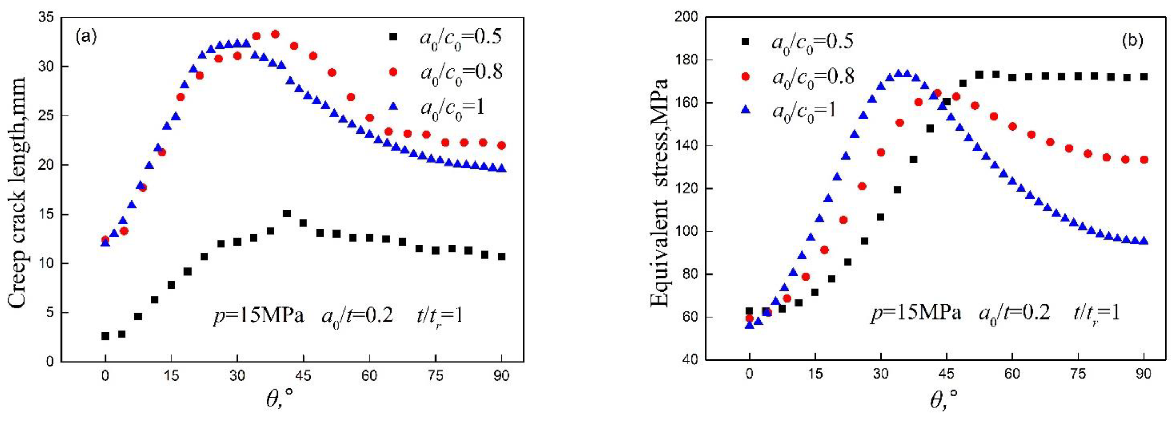
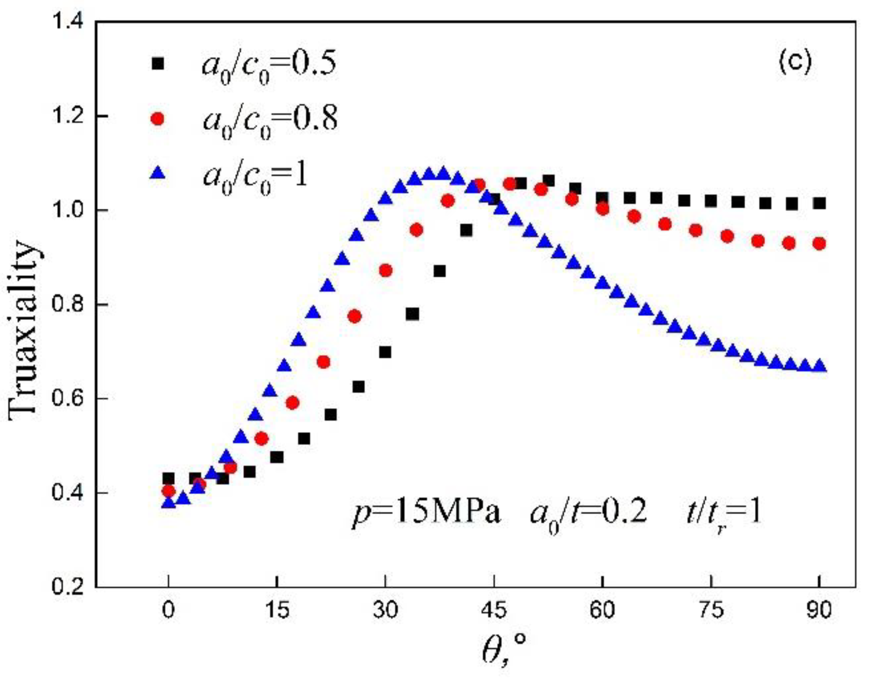
The initial crack shapes a0/c0 were assumed to be 0.5, 0.8, and 1, by turns, and were used to investigate the effect of the initial crack shape (a0/c0) on the creep crack growth behavior. The initial crack depth a0/t was assumed to be 0.2, and a 15 MPa internal pressure was applied. Figure 17 shows the damage distribution around the creep crack tip when t/tr = 1. The CCG lengths differ with the varying θ for each initial crack shape. The direction angles θ corresponding to the maximum creep crack length are about 42°, 38°, and 33°. Moreover, as a0/c0 = 0.5, the creep crack propagation lengths Δc (θ = 0°) and Δa (θ = 90°) and the maximum creep crack lengths are about 2.6 mm, 10.7 mm, and 15.1 mm, respectively. As a0/c0 = 0.8, the creep crack propagation lengths Δc (θ = 0°) and Δa (θ = 90°) and the maximum creep crack lengths are about 12.4 mm, 19.6 mm, and 32.8 mm, respectively. As a0/c0 = 1, the creep crack propagation lengths Δc (θ = 0°) and Δa (θ = 90°) and the maximum creep crack lengths are about 12.2 mm, 22.1 mm, and 33.1 mm, respectively. This indicates that the creep crack rate is greater at θ = 90° than at θ = 0°, the creep crack propagation length increases with the increasing initial crack shape a0/c0, and the CCG rate is faster when a0/c0 =1.
The creep crack length, the equivalent stress, and the stress triaxiality around the crack tip are shown in Figure 18a–c. The direction angles θ corresponding to the creep crack length, the maximum equivalent stress, and the stress triaxiality are about 42°, 38°, and 33° when a0/c0 is 0.5, 0.8, and 1, respectively. These results coincide with those in Figure 17. Therefore, these results indicate the same creep crack behavior by an axial surface crack with different initial crack shapes a0/c0.
5. Conclusions
In this paper, on the basis of the creep deformation constitutive model and the stress-dependent creep ductility model, the creep crack growth of P91 steel at 600 °C was simulated by FEM under a wide range of stress levels. The above model was also used to simulate the axial surface cracks in pressure pipes under different internal pressures, initial crack depth ratios (a0/t), and initial crack shapes (a0/c0). The main conclusions are as follows:
(1) Constitutive model Equation (12) was established on the basis of the creep deformation mechanism, in response to a wide range of stress levels and validated by comparing the simulated uniaxial tensile with the experimental data. The results showed that the primary and secondary creep deformation behaviors of the materials can be simulated accurately by the constitutive model Equation (12);
(2) With increasing , the transition region size of the creep ductility decreases. However, the effect of on the da/dt-C* curve can be neglected. With the increasing C*, the stress-dependent creep ductility for determining the CCG rate changes from the lower shelf value through a transition value to the upper shelf value. This change in the creep ductility values leads to three line segments of the da/dt-C* curve;
(3) Combining the constitutive model Equation (12) with stress-dependent creep ductility Equation (21), the CCG rate of P91 was calculated using different constitutive models in a wide stress region. The predicted results agree better with experimental data than the results of the other single-stress-regime constitutive model;
(4) The results of creep crack growth for the pressure pipes with the axial surface cracks showed that with an increase in internal pressure, the angle θ corresponding to the value of the maximum creep crack length changes from 64° to 33°. However, angle θ is almost independent of the initial crack depth ratios (a0/t) because of almost the same equivalent stress and triaxiality around the crack tip. Finally, the creep crack propagation length increases with the increasing initial crack shape (a0/c0) and the CCG rate is faster when a0/c0 = 1.
Author Contributions
Conceptualization, J.Z. (Jingwei Zhang) and J.L.; methodology, J.Z. (Jingwei Zhang) and J.L.; software, J.L.; validation, J.Z. (Jingwei Zhang) and Z.G.; formal analysis, J.Z. (Jingyi Zan); investigation, J.Z. (Jingyi Zan), J.L. and K.L.; data curation, Z.G.; writing—original draft preparation, J.Z. (Jingwei Zhang); writing—review and editing, J.Z. (Jingwei Zhang) and J.Z. (Jingyi Zan); visualization, J.Z. (Jingwei Zhang) and K.L.; supervision, K.L.; project administration, J.Z. (Jingwei Zhang) and K.L.; funding acquisition, J.Z. (Jingwei Zhang) All authors have read and agreed to the published version of the manuscript.
Funding
This research was funded by National Natural Science Foundation of China (No. 51705079), Natural Science Foundation of Fujian Province (No. 2018J01767), Quanzhou Science and Technology Department Project (2020G03).
Data Availability Statement
Not applicable.
Conflicts of Interest
The authors declare no conflict of interest.
References
- Nikbin, K.; Liu, S. Multiscale-constraint based model to predict uniaxial/multiaxial creep damage and crack growth in 316-H steels. Int. J. Mech. Sci. 2019, 156, 74–85. [Google Scholar] [CrossRef]
- Razak, N.A.; Davies, C.M.; Nikbin, K.M. Testing and assessment of cracking in P91 steels under creep-fatigue loading conditions. Eng. Fail. Anal. 2018, 84, 320–330. [Google Scholar] [CrossRef]
- Meng, Q.; Wang, Z. Extended finite element method for power-law creep crack growth. Eng. Fract. Mech. 2014, 127, 148–160. [Google Scholar] [CrossRef]
- Holdsworth, S. Advances in the assessment of creep data during the past 100 years. In Proceedings of the 9th Liege Conference: Materials for Advanced Power Engineering, Liege, Belgium, 27–29 September 2010; pp. 946–947. [Google Scholar]
- Payten, W. A reassessment of the multiaxial ductility C* creep crack growth equation based on the strain energy integral of the HRR singular field terms. Eng. Fract. Mech. 2019, 217, 106530. [Google Scholar] [CrossRef]
- Quintero, H.; Mehmanparast, A. Prediction of creep crack initiation behaviour in 316H stainless steel using stress dependent creep ductility. Int. J. Solids Struct. 2016, 97–98, 101–115. [Google Scholar] [CrossRef]
- Zhao, Y.; Gong, J.; Yong, J. Creep behaviour of P91/GTR-2CM/12Cr1MoV dissimilar joint predicted by the modified Theta method. Mater. High Temp. 2017, 34, 260–271. [Google Scholar] [CrossRef]
- Tan, J.P.; Wang, G.Z.; Xuan, F.Z.; Tu, S.T. Experimental investigation of in-plane constraint and out-of-plane constraint effect on creep crack growth. In Proceedings of the the ASME 2012 Pressure Vessels & Piping Division Conference, Toronto, ON, Canada, 15–19 July 2012. [Google Scholar]
- Zhang, J.W.; Wang, G.Z.; Xuan, F.Z.; Tu, S.T. The influence of stress-regime dependent creep model and ductility in the prediction of creep crack growth rate in Cr–Mo–V steel. Mater. Des. 2015, 65, 644–651. [Google Scholar] [CrossRef]
- Zhang, J.S. High Temperature Deformation and Fracture of Materials; Science Press: Beijing, China, 2007. [Google Scholar]
- Rieth, M.; Falkenstein, A.; Graf, P.; Heger, S.; Jäntsch, U.; Klimiankou, M.; Materna-Morris, E.; Zimmermann, H. Creep of the Austenitic Steel AISI 316L (N). Experiments and Models; Forhungcentrum Karlsruhe GmbH: Karlsruhe, Germany, 2004. [Google Scholar]
- Zhang, J.W. Numerical Prediction of Creep Crack Growth Rate and its Constraint Effect for a Wide Range of C*; East China University of Science and Technology: Shanghai, China, 2015. [Google Scholar]
- Zhang, J.W.; Wang, G.Z.; Xuan, F.Z.; Tu, S.T. Effect of stress dependent creep ductility on creep crack growth behaviour of steels for wide range of C*. Mater. High Temp. 2014, 32, 369–376. [Google Scholar] [CrossRef]
- Zhang, J.W.; Wang, G.Z.; Xuan, F.Z.; Tu, S.T. Prediction of creep crack growth behavior in Cr–Mo–V steel specimens with different constraints for a wide range of C*. Eng. Fract. Mech. 2014, 132, 70–84. [Google Scholar] [CrossRef]
- Oh, C.-S.; Kim, N.-H.; Kim, Y.-J.; Davies, C.; Nikbin, K.; Dean, D. Creep failure simulations of 316H at 550 °C: Part I—A method and validation. Eng. Fract. Mech. 2011, 78, 2966–2977. [Google Scholar] [CrossRef]
- He, J.Z.; Wang, G.Z.; Tu, S.T.; Xuan, F.Z. Characterization of 3-D creep constraint and creep crack growth rate in test specimens in ASTM-E1457 standard. Eng. Fract. Mech. 2016, 168, 131–146. [Google Scholar] [CrossRef]
- Wu, D.; Jing, H.; Xu, L.; Zhao, L.; Han, Y. Enhanced models of creep crack initiation prediction coupled the stress-regime creep properties and constraint effect. Eur. J. Mech. A/Solids 2019, 74, 145–159. [Google Scholar] [CrossRef]
- Gorash, Y.; Altenbach, H.; Lvov, G. Modelling of high-temperature inelastic behaviour of the austenitic steel AISI type 316 using a continuum damage mechanics approach. J. Strain Anal. Eng. Des. 2012, 47, 229–243. [Google Scholar] [CrossRef]
- Esposito, L.; Bonora, N.; de Vita, G. Creep modelling of 316H stainless steel over a wide range of stress. Procedia Struct. Integr. 2016, 2, 927–933. [Google Scholar] [CrossRef] [Green Version]
- Bonora, N.; Esposito, L. Mechanism Based Creep Model Incorporating Damage. J. Eng. Mater. Technol. 2010, 132, 021013. [Google Scholar] [CrossRef]
- Xue, J.-L.; Zhou, C.-Y.; Peng, J. Ultimate creep load and safety assessment of P91 steel pipe with local wall thinning at high temperature. Int. J. Mech. Sci. 2015, 93, 136–153. [Google Scholar] [CrossRef]
- Kimura, K.; Kushima, H.; Sawada, K. Long-term creep deformation property of modified 9Cr–1Mo steel. Mater. Sci. Eng. A 2009, 510–511, 58–63. [Google Scholar] [CrossRef]
- Liu, L.X. Research on Creep Property of 25Cr2NiMo1V Steel and FE Simulation on Constraint Effects; East China University of Science and Technology: Shanghai, China, 2009. [Google Scholar]
- Tan, J.P.; Tu, S.T.; Wang, G.Z.; Xuan, F.Z. Effect and mechanism of out-of-plane constraint on creep crack growth behavior of a Cr–Mo–V steel. Eng. Fract. Mech. 2013, 99, 324–334. [Google Scholar] [CrossRef]
- Robinson, E.L. Effect of temperature variation on the creep strength of steels. Trans. ASME 1938, 60, 253–259. [Google Scholar]
- Wen, J.-F.; Tu, S.-T.; Xuan, F.-Z.; Zhang, X.-W.; Gao, X.-L. Effects of Stress Level and Stress State on Creep Ductility: Evaluation of Different Models. J. Mater. Sci. Technol. 2016, 32, 695–704. [Google Scholar] [CrossRef]
- ASTM E 1457; Standard Test Method for Measurement of Creep Crack Growth Rates in Metals. Annual Book of ASTM Standards: West Conshohocken, PA, USA, 2001; Volume 3, pp. 945–966.
- Wen, J.-F.; Tu, S.-T. A multiaxial creep-damage model for creep crack growth considering cavity growth and microcrack interaction. Eng. Fract. Mech. 2014, 123, 197–210. [Google Scholar] [CrossRef]
- McClintock, F.A. A criterion for ductile fracture by the growth of holes. J. Appl. Mech. 1968, 35, 363–371. [Google Scholar] [CrossRef]
- Rice, J.R.; Tracey, D.M. On the ductile enlargement of voids in triaxial stress fields. J. Mech. Phys. Solids 1969, 17, 201–217. [Google Scholar] [CrossRef] [Green Version]
- Cocks, F.A.C.; Ashby, F.M. Intergranular fracture during power-law creep under multiaxial stresses. Met. Sci. 1980, 9, 395–402. [Google Scholar] [CrossRef]
- Spindler, M.W. The multiaxial and uniaxial creep ductility of Type 304 steel as a function of stress and strain rate. Mater. High Temp. 2004, 21, 47–54. [Google Scholar] [CrossRef]
- Zhou, Y.; Xuedong, C.; Fan, Z.; Yichun, H. An improved mechanism-based creep constitutive model using stress-dependent creep ductility. In Proceedings of the ASME 2016 Pressure Vessels and Piping Conference, American Society of Mechanical Engineers Digital Collection, Vancouver, BC, Canada, 17–21 July 2016. [Google Scholar]
- Gorash, Y. Development of a Creep-Damage Model for Non-Isothermal Long-Term Strength Analysis of High-Temperature Components Operating in a Wide Stress Range. Ph.D. Thesis, Martin-Luther-Universitat Halle-Wittenberg, Kharkiv, Ukraine, 2008. [Google Scholar]
- Kloc, L.; Sklenička, V. Transition from power-law to viscous creep behaviour of p-91 type heat-resistant steel. Mater. Sci. Eng. A 1997, 234–236, 962–965. [Google Scholar] [CrossRef]
- Kloc, L.; Sklenička, V. Confirmation of low stress creep regime in 9% chromium steel by stress change creep experiments. Mater. Sci. Eng. A 2004, 387–389, 633–638. Mater. Sci. Eng. A 2004, 387–389, 633–638. [Google Scholar] [CrossRef]
- Sklenicka, V.; Kucharova, K.; Kudrman, J.; Svoboda, M.; Kloc, L. Microstructure stability and creep behaviour of advanced high chromium ferritic steels. Kov. Mater. Met. Mater. 2005, 43, 20–33. [Google Scholar]
Figure 1.
True stress–strain curve of the P91 steel at 600 °C [21].
Figure 1.
True stress–strain curve of the P91 steel at 600 °C [21].

Figure 2.
Round bar sample in the uniaxial creep simulation.
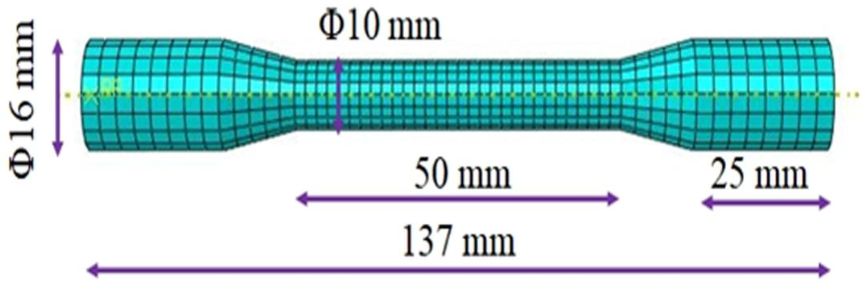
Figure 3.
The geometry of the CT specimen (mm).
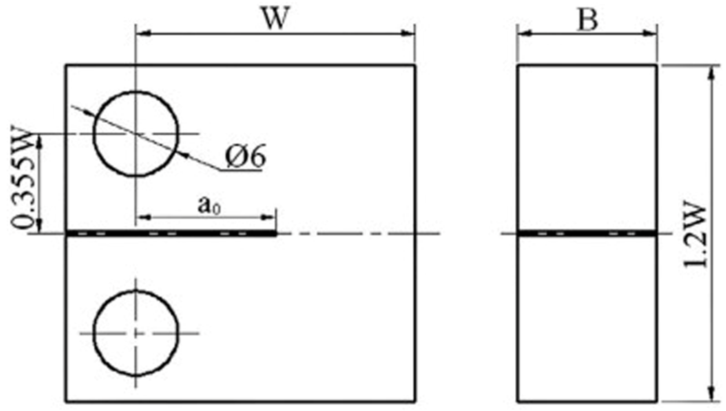
Figure 4.
The FE meshes of the whole CT specimen (a) and local meshes at the crack tip (b).

Figure 5.
Creep ductility against the normalized stress in the Nikbin model [1,34] (a) and the four-parameter model [33,34] (b).
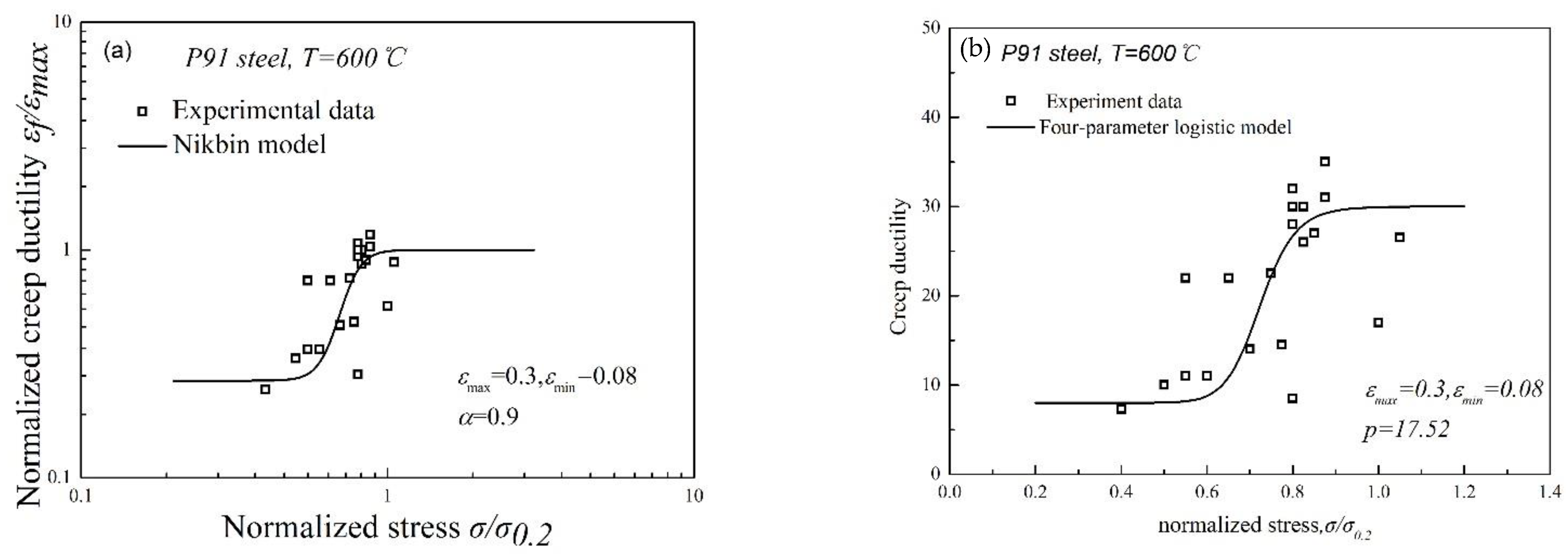
Figure 6.
Uniaxial tension test under different stress levels [22].
Figure 6.
Uniaxial tension test under different stress levels [22].
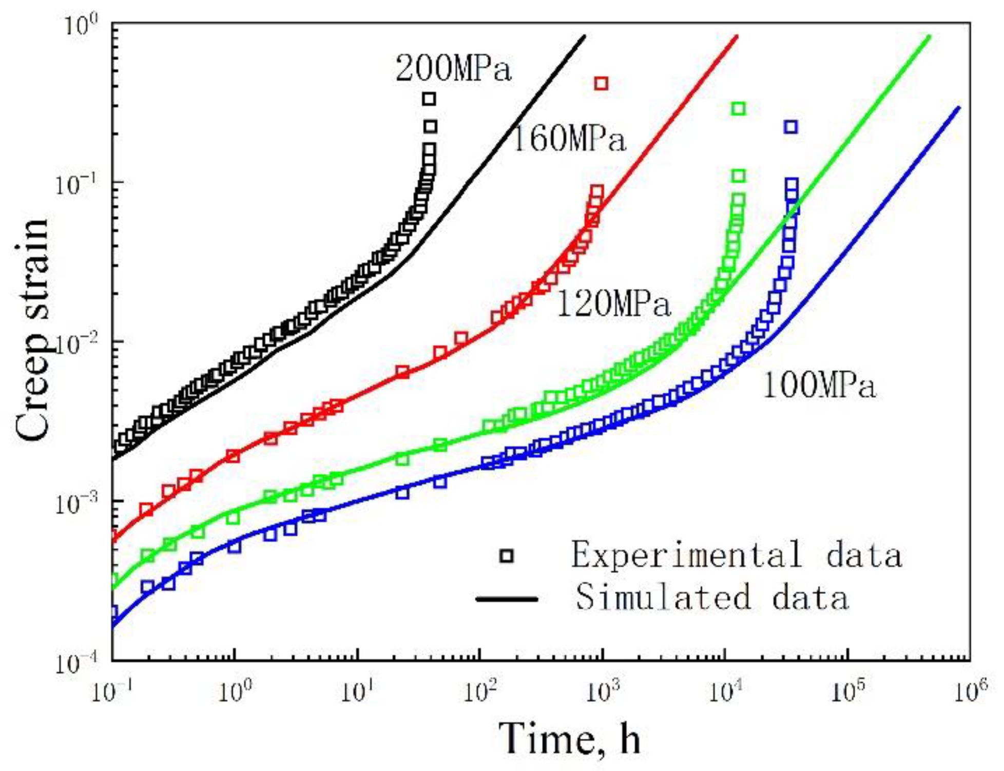
Figure 7.
Different parameter α in the creep ductility model [34].
Figure 7.
Different parameter α in the creep ductility model [34].
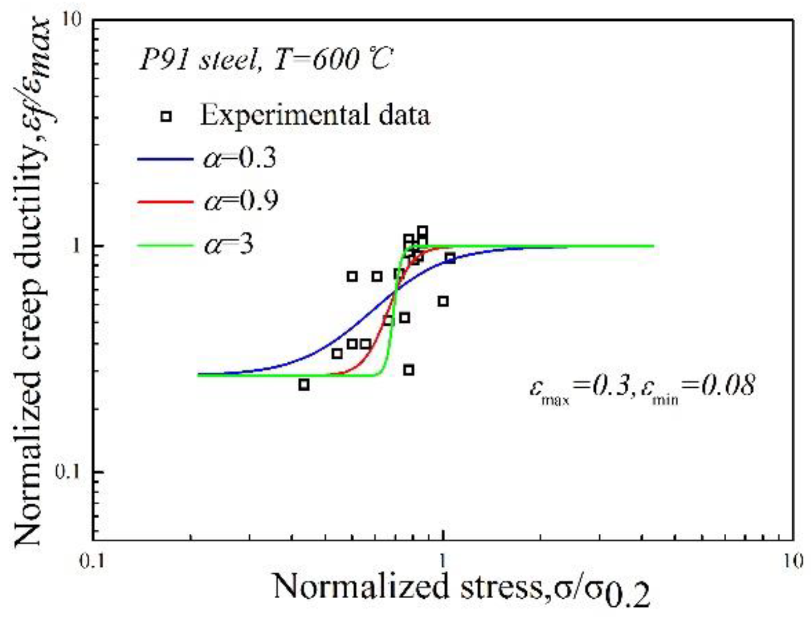
Figure 8.
The effect of parameter α in the creep ductilities on the CCG rates.


Figure 10.
The da/dt-C* correlation curves calculated by: the Norton model (a), the 2RN model (b), the sine-hyperbolic model (c) and the Equation (12) constitutive model (d) in a wide range of C* and a comparison with the experimental da/dt-C* curves [5].
Figure 10.
The da/dt-C* correlation curves calculated by: the Norton model (a), the 2RN model (b), the sine-hyperbolic model (c) and the Equation (12) constitutive model (d) in a wide range of C* and a comparison with the experimental da/dt-C* curves [5].
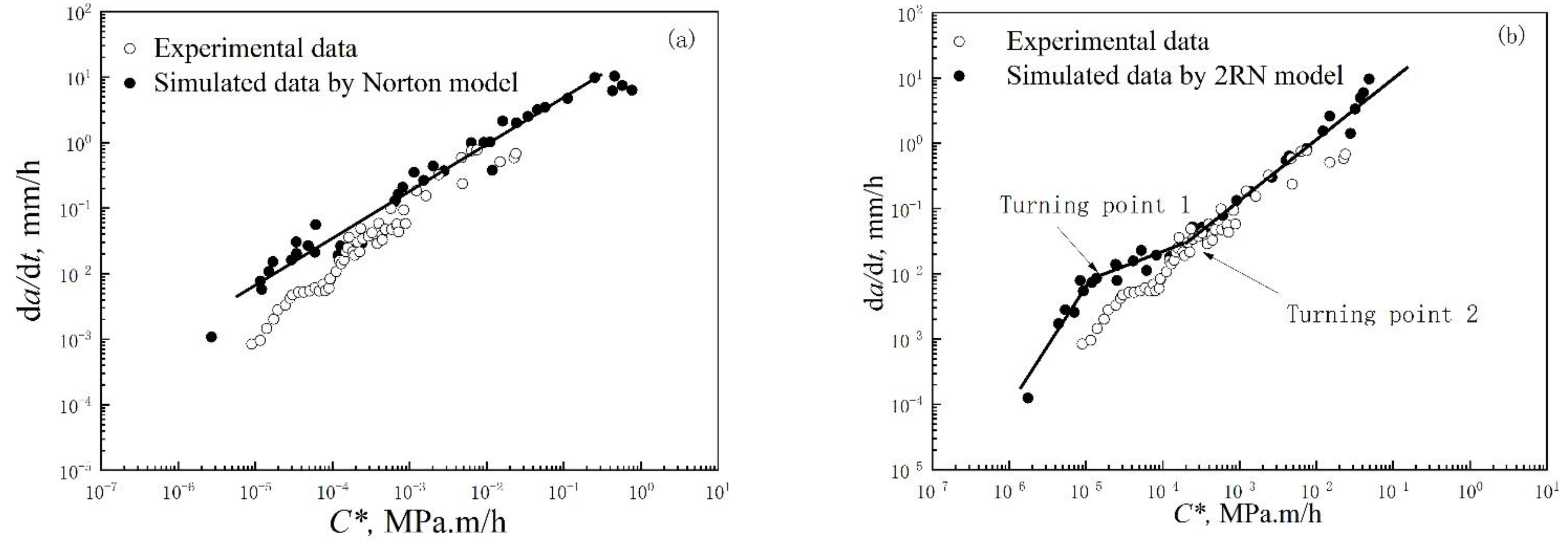
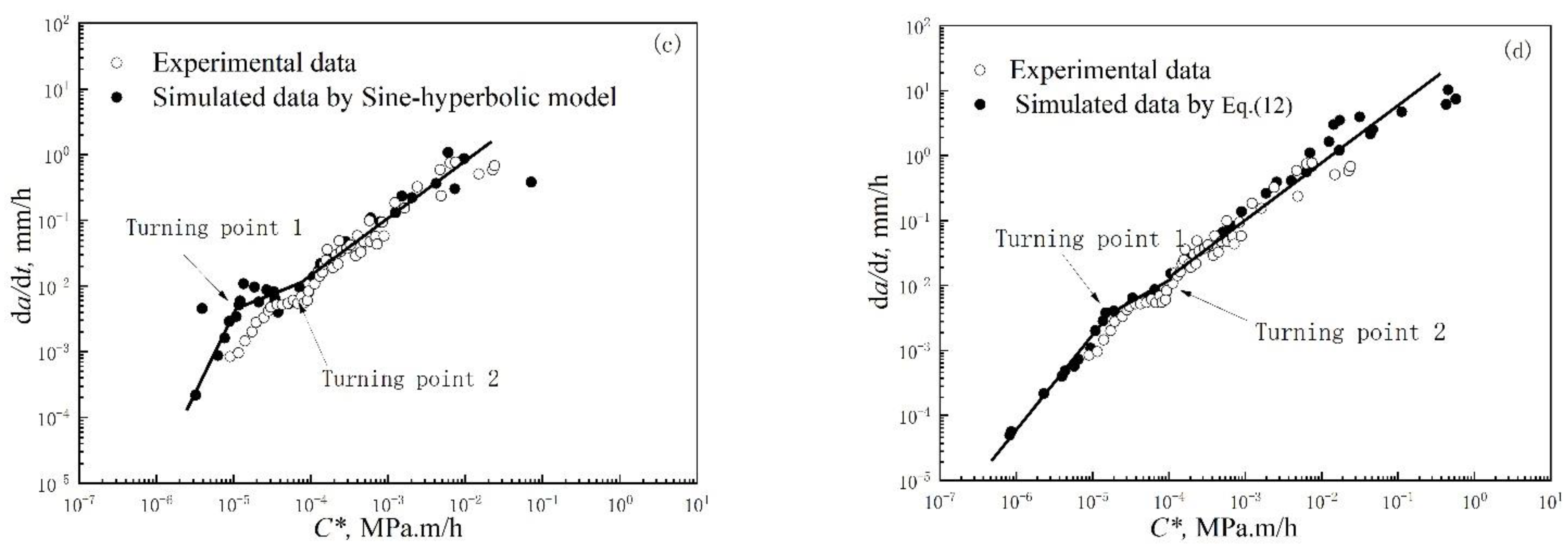
Figure 11.
The schematic diagram of (a) pressurized pipes with an axial surface crack and (b) an axial surface crack.
Figure 11.
The schematic diagram of (a) pressurized pipes with an axial surface crack and (b) an axial surface crack.

Figure 12.
The FE model (a) and local mesh distribution around the crack tip (b).

Figure 13.
The distribution of the damage around the creep crack tip (a) p = 5 MPa, (b) p = 10 MPa and (c) p = 15 MPa.
Figure 13.
The distribution of the damage around the creep crack tip (a) p = 5 MPa, (b) p = 10 MPa and (c) p = 15 MPa.

Figure 14.
The relationship between the creep crack propagation length and θ.
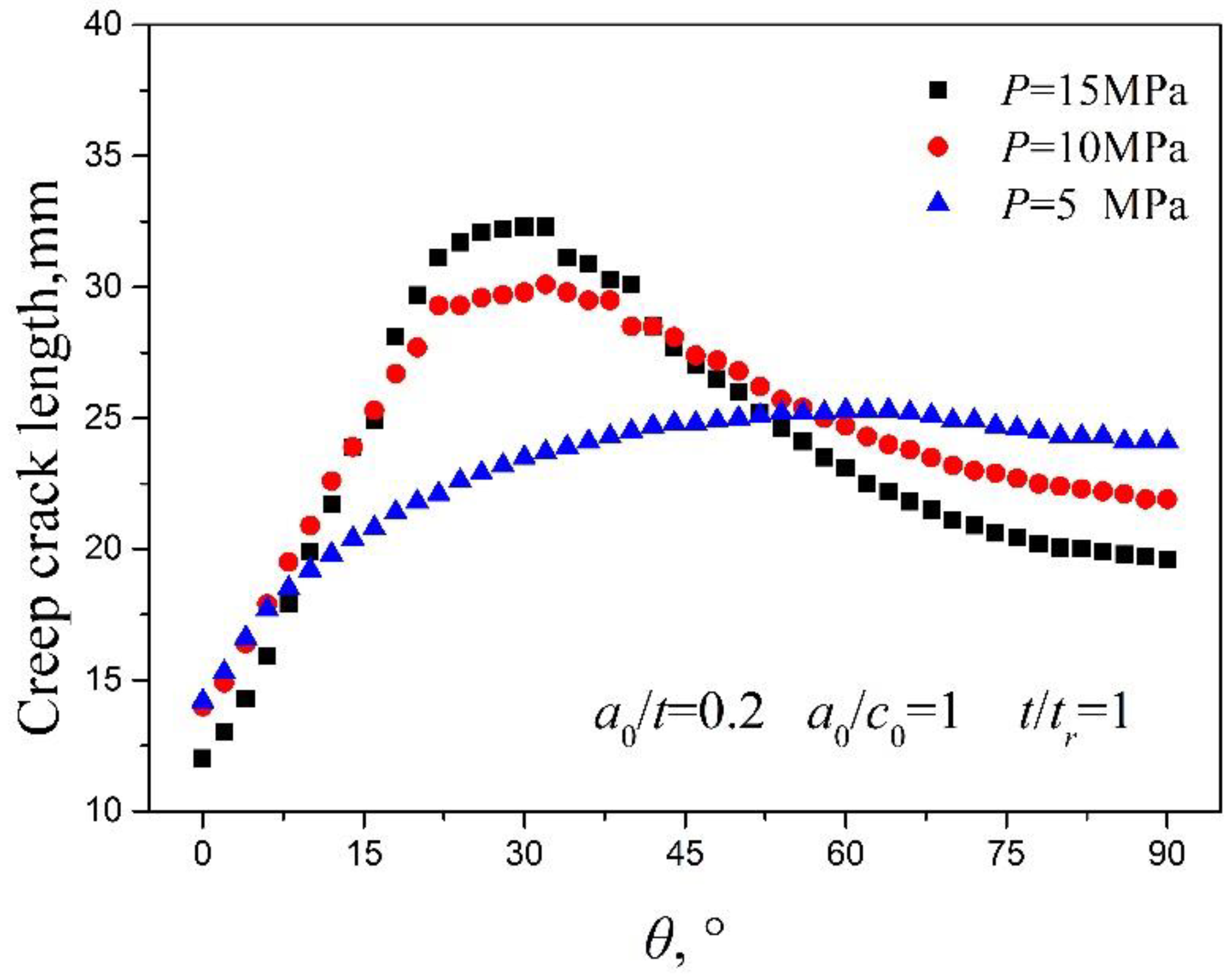
Figure 15.
The damage distribution around the creep crack tip (a) a0/t = 0.2, (b) a0/t = 0.3 and (c) a0/t = 0.4.
Figure 15.
The damage distribution around the creep crack tip (a) a0/t = 0.2, (b) a0/t = 0.3 and (c) a0/t = 0.4.

Figure 16.
The relationship between the (a) creep crack length, (b) equivalent stress, (c) triaxiality and θ.
Figure 16.
The relationship between the (a) creep crack length, (b) equivalent stress, (c) triaxiality and θ.
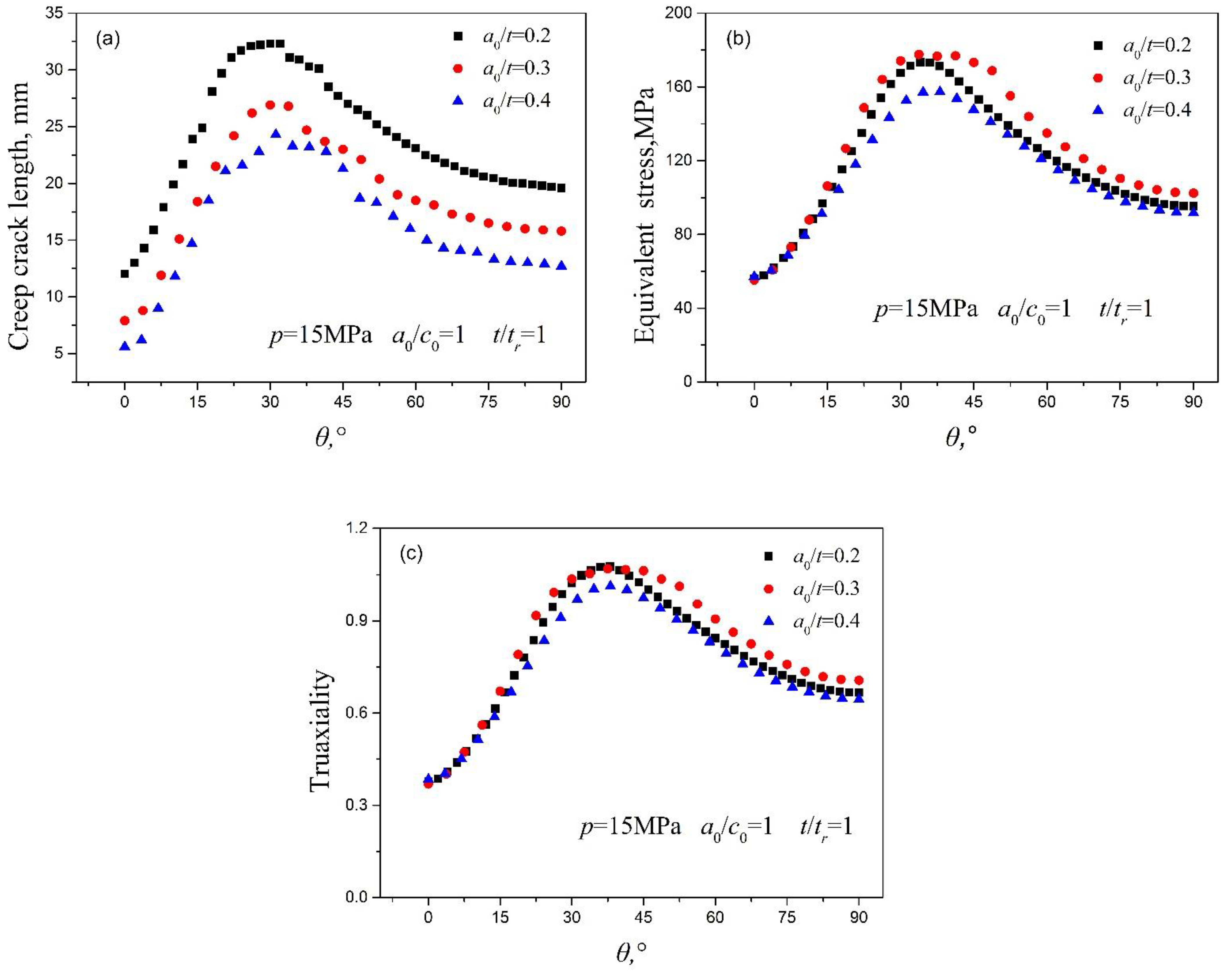
Figure 17.
The damage distribution around the creep crack tip (a) a0/c0 = 0.5, (b) a0/c0 = 0.8 and (c) a0/c0 = 1.
Figure 17.
The damage distribution around the creep crack tip (a) a0/c0 = 0.5, (b) a0/c0 = 0.8 and (c) a0/c0 = 1.

Figure 18.
The relationship between the (a) creep crack length, (b) equivalent stress, (c) triaxiality and θ.
Figure 18.
The relationship between the (a) creep crack length, (b) equivalent stress, (c) triaxiality and θ.

Table 1.
Chemical composition of the P91 steel (wt%).
| C | Mn | Si | Cr | Ni | Mo | V | Nb | N | Al | Ti | Fe |
|---|---|---|---|---|---|---|---|---|---|---|---|
| 0.108 | 0.457 | 0.221 | 9.09 | 0.217 | 0.991 | 0.206 | 0.078 | 0.047 | 0.012 | 0.005 | Bal |
Table 2.
Parameters in the constitutive models.
| Model | Mathematical Formulation |
|---|---|
| Norton | |
| 2RN | |
| Sine-hyperbolic model | |
| Equation (12) constitutive model |
Publisher’s Note: MDPI stays neutral with regard to jurisdictional claims in published maps and institutional affiliations. |
© 2022 by the authors. Licensee MDPI, Basel, Switzerland. This article is an open access article distributed under the terms and conditions of the Creative Commons Attribution (CC BY) license (https://creativecommons.org/licenses/by/4.0/).
Share and Cite
MDPI and ACS Style
Zhang, J.; Li, J.; Zan, J.; Guo, Z.; Liu, K. A Creep Constitutive Model, Based on Deformation Mechanisms and Its Application to Creep Crack Growth. Metals 2022, 12, 2179. https://doi.org/10.3390/met12122179
AMA Style
Zhang J, Li J, Zan J, Guo Z, Liu K. A Creep Constitutive Model, Based on Deformation Mechanisms and Its Application to Creep Crack Growth. Metals. 2022; 12(12):2179. https://doi.org/10.3390/met12122179
Chicago/Turabian StyleZhang, Jingwei, Jie Li, Jingyi Zan, Zijian Guo, and Kanglin Liu. 2022. "A Creep Constitutive Model, Based on Deformation Mechanisms and Its Application to Creep Crack Growth" Metals 12, no. 12: 2179. https://doi.org/10.3390/met12122179
Note that from the first issue of 2016, this journal uses article numbers instead of page numbers. See further details here.