Dynamic Load Identification of Unspecified Metal Structures by Measuring Their Response

Abstract

Many engineering structures are made of metal composite materials. External load information is a key issue for the design and condition monitoring of the structures. Due to the limitation of measurement technology and the external environment, it is difficult to directly measure dynamic loads on structures in many circumstances. This paper focuses on evaluating the external load applied on a structure with unknown dynamic properties. We proposed a novel dynamic load identification method that is based on the Bayesian principle coupled with the extended Kalman filter method. Firstly, the modal parameters are identified under ambient excitation using the Bayesian fast Fourier transform method (FFT). The posterior probability density function (PDF) and covariance of the modal parameters are obtained by the Fourier transform of the response data, and then the modal parameters of the structure are obtained based on unconstrained optimization. Next, the extended Kalman filter method in the modal space is used to update the modal parameters and identify the time-domain information of dynamic loads. The accuracy of the proposed theory was evaluated experimentally using a Bernoulli−Euler beam. The results showed that the method is feasible and efficient.

1. Introduction

Identifying the dynamic load acting on a metal structure is essential for a large variety of applications. For example, dynamic loads applied on a structure are responsible for the majority of failures during service [1,2,3,4]. Therefore, to improve the safety and the reliability of a structure, it is not enough to ensure that the static characteristics meet the design requirements. Dynamic loads should also be closely monitored in order to ensure that they do not exceed certain limits.

Current dynamic loads identification methods are mostly based on specified systems with known parameters, e.g., the stiffness and the damping [5,6,7]. These parameters are usually identified by applying artificial excitations. However, in many cases, this identification method may affect the normal operation of a structure (such as bridges and rotors in operation) [8,9]. Such artificial excitation may also cause structural damage. A practical approach to obtaining modal parameters is ambient vibration tests (AVTs) [10,11], which are usually economical and time-saving. Several modal parameter identification methods based on ambient excitation, such as the lbrahim time domain technique (ITD) [12], the autoregressive moving average model (ARMA) [13], and the random subspace method [14], are available in the literature. Among these approaches, the fast Fourier transform modal parameter identification method based on Bayesian probability [15,16] is the most efficient, as it makes full use of the response data and obtains the modal priori parameters. Furthermore, in the presence of noise, the identification results are often more accurate than other methods thanks to the Bayesian probability principle.

In the field of dynamic load identification, among Bayesian methods we have the Bayesian regularization method [17] and the Bayesian particle filter method [18]. Furthermore, the Kalman filter method [19] can also be considered as a special case of Bayesian methods where the Kalman filter is usually combined with the least square method [20]. Zhang et al. [21] used the Bayesian method to reconstruct a structural load with measurement noise and model uncertainty. Yan [22] identified the impact load on a composite plate by the Bayesian regularization method, and they also used the Kalman filter algorithm to identify the impact position. Faure et al. [23] used the Bayesian regularization method to identify the load position by assessing the displacement response. This method does not need the boundary conditions but is highly sensitive to the noise in the response measurement. The Kalman filter is developed in the modern control theory and has been successfully applied in the field of dynamic load identification. When considering a dynamic model that contains a Gaussian model error and the response signal is corrupted by a Gaussian noise, the Kalman filter load identification method [24,25,26,27,28] can accurately reconstruct the time-domain information of the load in both the physical space and the modal space. Several scholars have proposed the extended Kalman filter [20,29,30] and the unscented Kalman filter [27,31] to correct these errors and to identify loads. Lourens [25] proposed the extended Kalman filter to identify the load, which extends the unknown force vector to the state vector to form the augmented state vector, and uses the Kalman filter to identify the augmented state vector so as to identify the load. Naets et al. [26] studied the observability of this method and pointed out that the system is unobservable when only the acceleration response is used to identify the load. In order to solve this problem, they combined the virtual displacement technology with the acceleration response and improved the Kalman filter to identify the load. Yang et al. [27,28,29] composed the state vector and the model parameters into an augmented state vector. They used the extended Kalman filter to identify the augmented state vector and employed complex mathematical equations to identify the load.

The methods mentioned above are all based on the assumption of known system parameters. However, it remains to be studied how to identify the load when only the response data are known for an unspecified system under a random excitation. Moreover, these methods are only developed in the physical space and not in the modal space, which can lead to complicated computation when applied to large-scale structures. Developing a similar approach for the modal space is useful for large-scale engineering structures. In this paper, we firstly introduced the extended Kalman filter method into the modal space to identify the modal parameters and load of unspecified systems using only random excitation response data.

This paper is organized as follows: In Section 1, the introduction of the research background is described. In Section 2, the posterior PDF and covariance of modal parameters were obtained by the Fourier transform of the response data. Then, the modal parameters of the structure were obtained based on unconstrained optimization (Section 2.1). The extended Kalman filter load identification method in the modal space was derived to update the modal parameters with errors and identify the excitation (Section 2.2). In Section 3, a 3-DOF structure was simulated to verify the correctness of the extended Kalman filter. A simply supported beam under random loads was used to demonstrate the effectiveness and feasibility of the proposed methods in Section 2. Finally, the conclusions are presented in Section 5.

2. Dynamic Load Identification Method

The method proposed in this paper includes two stages:

Firstly, a Bayesian method is used to identify the modal parameters of the structure under ambient excitation. Secondly, the extended Kalman filter method is used to update the modal parameters and identify the time-domain information of the dynamic loads. Research manuscripts reporting large datasets that are deposited in a publicly available database should specify where the data have been deposited and provide the relevant accession numbers. If the accession numbers have not yet been obtained at the time of submission, please note that they will be provided during review. They must be provided prior to publication.

2.1. Bayesian FFT Modal Identification

In this section we introduced a multi-modal identification method based on Bayesian principle, which is a forward problem. The parameters optimal result was derived using the probability, while the rationality of the results was measured by the variance. It should be mentioned that the Bayesian method for multi-modal identification has the disadvantages of needing complex calculations and often involving large errors especially when considering high modal orders, i.e., orders exceed three. However, this is not the case in a single-mode identification. In this paper, the single-mode identification method was introduced.

We start by defining the vector $\left\{y_j\right\}$, where $\{y_j\in R^n:j=1,\cdots N\}$ is the acceleration time history measured at $n$ DOFs of a structure. The number of sampling points per channel is N. The FFT of $\left\{y_j\right\}$ can then be defined as:

$$Y_k=F_k+\mathrm{i}{G}_k=\sqrt{(2\Delta t)/N}{\displaystyle \sum _{j=1}^N{y}_j}\exp \{-2\pi \mathrm{i}[(k-1)(j-1)/N]\}(k=1,\cdots N),$$

(1)

where $i^2=-1$; $F_k=\mathrm{Re}{Y}_k \mathrm{and} G_k=\mathrm{Im}{Y}_k$ are the real and imaginary parts of the FFT, respectively; and $\Delta t$ is the sampling interval. The FFT corresponds to the frequency $f_k=(k-1)/N\Delta t$ for $k=2,3\cdots N_d$, where $N_d=\mathrm{int}[N/2]+1$ is the number of frequencies used for the FFT. The scaling factor of the FFT makes the spectral density matrix unilateral invertible, and the frequency is measured in Hz. The frequency resolution after being converted to the frequency domain is $\Delta f=1/N\Delta t$.

The modal parameters $\theta$ to be identified include the modal frequency $f$, the modal damping ratio $\zeta$, the modal mode shape $\Phi$, the cross-spectral density of the modal excitation $S_{ij}$, and the spectral density of the prediction error ${\sigma }^2$. Let $\widehat{\theta }$ be the most probable value (MPV). The posterior PDF of $\theta$ is proportional to the likelihood function $p(\{Z_k\}|\theta )$:

$$\begin{array}{c}p\left(\theta |\left\{Z_k\right\}\right)\propto p\left(\left\{Z_k\right\}|\theta \right)={\left(2\pi \right)}^{-\left(N_q-1\right)/2}{\left[{\displaystyle \prod _{k=2}^{N_q}\det C_k\left(\theta \right)}\right]}^{-1/2}\\ \times \exp \left[-\left(1/2\right){\displaystyle \sum _{k=2}^{N_q}{Z}_k^T{C}_k\left(\theta \right)Z_k}\right]\end{array}$$

(2)

where

$$Z_k={\left[F_k^T,G_k^T\right]}^T\in R^{2N_s}:k=2,\cdots ,N_d,$$

(3)

$C_k$ is the covariance matrix of $Z_k$ [31] and described as:

$$C_k=\frac{1}{2}\left[\begin{array}{cc}\Phi (\mathrm{Re}{H}_k){\Phi }^T& \Phi {(\mathrm{Im}{H}_k)}^T{\Phi }^T\\ \Phi (\mathrm{Im}{H}_k){\Phi }^T& \Phi (\mathrm{Re}{H}_k){\Phi }^T\end{array}\right]+\frac{{\sigma }^2}{2}{I}_{2n},$$

(4)

$H_k$ is the spectral density matrix of the model response with ${\beta }_{ik}=f_i/f_k$ and written as:

$$H_k(i,j)=S_{ij}{\left[({\beta }_{ik}^2-1)+i(2{\zeta }_i{\beta }_{ik})\right]}^{-1}{\left[({\beta }_{jk}^2-1)+i(2{\zeta }_j{\beta }_{jk})\right]}^{-1},$$

(5)

$f_i$ and ${\zeta }_i$ are the natural frequency and the damping ratio of the $i$th mode, respectively; $S_{ij}$ is the cross spectral density between the $i$th- and $j$th-mode excitations. For convenience, Equation (2) is rewritten as:

$$p\left(\theta |\left\{Z_k\right\}\right)\propto \exp \left[-L\left(\theta \right)\right],$$

(6)

$$L(\theta )=\frac{1}{2}{\displaystyle \sum _{k=2}^{N_q}\left[\ln \det C_k(\theta )+Z_k^T{C}_k{(\theta )}^{-1}{Z}_k\right]}.$$

(7)

When the sampling data are large enough, the posterior PDF can be represented as a Gauss distribution:

$$p\left(\theta |\left\{Z_k\right\}\right)\propto \exp \left[-\frac{1}{2}{(\theta -\widehat{\theta })}^{\mathrm{T}}{\widehat{C}}^{-1}(\widehat{\theta })(\theta -\widehat{\theta })\right],$$

(8)

$$\widehat{C}=H_L{(\widehat{\theta })}^{-1},$$

(9)

where $H_L(\widehat{\theta })$ is the Hessian of $L$ at the most optimal parameter value [27].

If all modes are completely separated and a selected frequency bandwidth contains only a single mode, a single-mode identification method can be used in this bandwidth. The FFT data of the selected bandwidth contain all the modal parameters of that mode. Modal parameter $\theta$ consists of the natural frequency $f$, the damping ratio $\zeta$, the mode shape $\phi \in R^n$, the spectral density of the modal excitation $S$, and the spectral density of the prediction error ${\sigma }^2$.

Next, $L(\theta )$ is given by:

$$\begin{array}{c}L(f,\zeta ,S,{\sigma }^2,\phi )=-n{N}_f\ln 2+(n-1)N_f\ln {\sigma }^2\\ +{\displaystyle \sum _k\ln (S{D}_k+{\sigma }^2)}+{\sigma }^{-2}(d-{\Phi }^{T}A\Phi )\end{array}$$

(10)

where $N_f$ is the total number of the sampling points in the selected bandwidth,

$$D_k={\left[{\left({\beta }_k^2-1\right)}^2+{\left(2\zeta {\beta }_k\right)}^2\right]}^{-1},$$

(11)

$$A={{\displaystyle \sum _k[1+({\sigma }^2/S{D}_k)]}}^{-1}{D}_k,$$

(12)

$$D_k=F_k{F}_k^T+G_k{G}_k^T,$$

(13)

$$d={\displaystyle \sum _k(F_k^T{F}_k+G_k^T{G}_k)}=trace(A_0),$$

(14)

$$A_0={\displaystyle \sum _k{D}_k}.$$

(15)

The sum in the equation adds $N_f$ terms of the bandwidth of the selected frequency. The most probable value (MPV) of the mode vector $\phi$ is the eigenvector corresponding to the maximum eigenvalue of $A$. Then, the unit normalization of the mode vector is carried out as $\phi /\Vert \phi \Vert$, ${\Vert \phi \Vert }^2={\phi }^T\phi$. Minimizing with respect to $\phi$ leads to $L$ being only dependent on the remaining four parameters:

$$\begin{array}{l}L(f,\zeta ,S,{\sigma }^2)=-n{N}_f\ln 2+(n-1)N_f\ln {\sigma }^2\\ +{\displaystyle \sum _k\ln (S{D}_k+{\sigma }^2)}+{\sigma }^{-2}(d-\widehat{\lambda })\end{array}$$

(16)

where $\widehat{\lambda }$ is the largest eigenvalue of $A$. The MPV of the four remaining parameters can be obtained using an unconstrained numerical optimization approach. To this end, we define the following factor as the signal-to-noise ratio at the frequency $f_k$:

$${\gamma }_k=S{D}_k/{\sigma }^2.$$

(17)

In the selected bandwidth, if ${\gamma }_k>>1$, the following relationship can be obtained:

$${(1+{\gamma }_k{}^{-1})}^{-1}={[1+({\sigma }^2/S{D}_k)]}^{-1}~1-({\sigma }^2/S{D}_k)~1.$$

(18)

Using the zero-order approximation, the matrix $A$ becomes:

$$A~{\displaystyle \sum _k{D}_k=A_0},$$

(19)

which is a constant matrix. Then, the MPV of $\phi$ can be obtained from Equation (19), while the MPV of ${\sigma }^2$ and $S$ can also be found as:

$${\widehat{\sigma }}^2=(d-{\widehat{\lambda }}_0)/(n-1)N_f,$$

(20)

$$\widehat{S}(f,\varsigma )=N_f^{-1}{\displaystyle \sum _k{D}_k}{(f,\varsigma )}^{-1}{\widehat{D}}_k,$$

(21)

where

$${\widehat{\lambda }}_0={\widehat{\phi }}^T{A}_0\widehat{\phi },$$

(22)

$${\widehat{D}}_k={\widehat{\phi }}^T{D}_k\widehat{\phi }.$$

(23)

Thus, we see that $L$ depends only on the remaining parameters $f$ and $\zeta$:

$$L(f,\zeta )\sim {\displaystyle \sum _k\ln D_k}(f,\zeta )+N_f\ln [N_f^{-1}{\displaystyle \sum _k{D}_k{(f,\zeta )}^{-1}{\widehat{D}}_k}]+\mathrm{const}.$$

(24)

The steps to obtain modal parameters of a single mode can be summarized as:

• Calculate the FFT of the sequence $\left\{F_k,G_k\right\}$ and then evaluate the matrices $D_k$ using Equation (13) and the matrix $A_0$ using Equation (19);
• Calculate the MPV as the eigenvector of $A_0$ using the largest eigenvalue and then the MPV of ${\sigma }^2$ using Equation (20);
• Numerically optimize Equation (24) with respect to $f$ and $\zeta$. The initial guess for $f$ can be obtained from the FFT spectrum of the response. The initial guess of $\zeta$ may be set to 1%. Then, the MPV of $S$ can be obtained from Equation (21).

2.2. Dynamic Load Identification Method Based on Extended Kalman Filter in the Modal Space

The equation of motion for a dynamic system can be expressed as a set of ordinary differential equations:

$$M\ddot{p}(t)+C\dot{p}(t)+Kp(t)=B_{f}f(t),$$

(25)

where $f(t)$ is the excitation vector with $B_f\in R^{n\times r}$ being the matrix of the excitation positions composed of ones and zeros. Ones are used at the degrees of freedom corresponding to the excitation locations and zeros everywhere else. $M$, $C$, and $K$ denote the mass, damping, and stiffness matrix, respectively. The state space model of the dynamic system, i.e., the equation of state and the equation of observation, can be written as Equations (26) and (27), respectively:

$$\dot{x}(t)=\left[\begin{array}{c}\dot{p}(t)\\ \ddot{p}(t)\\ \dot{\mathsf{\theta }}\end{array}\right]+w(t)=\left[\begin{array}{c}\dot{p}(t)\\ M^{-1}\left[B_{f}f(t)-C_{\theta }\dot{p}(t)-K_{\theta }p(t)\right]\\ [0]\end{array}\right]+w(t)=g(x(t),f(t))+w(t),$$

(26)

$$y(t)=H_0\ddot{p}(t)+v(t)=h(x(t),f(t))+v(t),$$

(27)

where $g$ and $h$ are non-linear functions, $x(t)={\left[\begin{array}{ccc}p(t)& \dot{p}(t)& \theta \end{array}\right]}^T$ is the augmented state vector, $p(t)$ is the displacement vectors, $\theta =\left[\begin{array}{cccc}{\theta }_1& {\theta }_2& \cdots & {\theta }_s\end{array}\right]$ is the modal parameter vectors, $y(t)$ is the acceleration vector of the observation point, $w(t)$ and $v(t)$ are the model noise and the observation noise, respectively, the variances are $G_k$ and $R_k$, and $H_0$ is the observation vectors.

Discretizing the above nonlinear equations in the time domain, we obtain:

$${\dot{x}}_k=g(x_k,f_k)+w_k,$$

(28)

$$\begin{array}{l}{y}_k=h(x_k,f_k)+v_k=H_0{\ddot{p}}_k+v_k=H_0{M}^{-1}\left[B_f{f}_k-C_{\theta }{\dot{p}}_k-K_{\theta }{p}_k\right]+v_k\\ =\overline{h}(x_k)+H_0{M}^{-1}{B}_f{f}_k+v_k=\overline{h}(x_k)+D_k{f}_k+v_k\end{array}$$

(29)

Applying the first-order Taylor expansion to the non-linear functions $g$ and $h$, we arrive at the following approximate linear functions:

$$g_k(x_k,f_k)\approx g_k(E(x_k),f_k)+\frac{\partial g(x,f)}{\partial x}{|}_{x_{k|k},f_k}·\left(x_k-E(x_k)\right)+\frac{\partial g(x,f)}{\partial f}{|}_{x_{k|k},f_k}·\left(f_k-E\left(f_k\right)\right),$$

(30)

$$h_k(x_k,f_k)\approx h_k(E(x_k),f_k)+\frac{\partial h(x,f)}{\partial x}{|}_{x_{k|k},f_k}·\left(x_k-E(x_k)\right),$$

(31)

with

$$\begin{array}{l}\frac{\partial g(x,f)}{\partial x}{|}_{x=x_{k|k},f=f_k}=\left[\begin{array}{ccc}\frac{\partial g}{\partial p}& \frac{\partial g}{\partial \dot{p}}& \frac{\partial g}{\partial \theta }\end{array}\right]\\ =\left[\begin{array}{ccccc}\left[0\right]& I& \left[0\right]& \cdots & \left[0\right]\\ -M^{-1}{K}_{\theta }& -M^{-1}{C}_{\theta }& -M^{-1}\frac{\partial K_{\theta }}{\partial {\theta }_1}{p}_{k|k}-M^{-1}\frac{\partial C_{\theta }}{\partial {\theta }_1}{\dot{p}}_{k|k}& \cdots & -M^{-1}\frac{\partial K_{\theta }}{\partial {\theta }_s}{p}_{k|k}-M^{-1}\frac{\partial C_{\theta }}{\partial {\theta }_s}{\dot{p}}_{k|k}\\ \left[0\right]& \left[0\right]& \left[0\right]& \cdots & \left[0\right]\end{array}\right]=A\end{array}$$

(32)

$$\frac{\partial g(x,f)}{\partial f}{|}_{x=x_{k|k},f=f_k}=\left[\begin{array}{c}\left[0\right]\\ M^{-1}{B}_f\\ \left[0\right]\end{array}\right]=B,$$

(33)

$$\begin{array}{l}\frac{\partial h(x,f)}{\partial x}{|}_{x=x_{k|k-1},f_k}=\left[\begin{array}{ccc}\frac{\partial h}{\partial p}& \frac{\partial h}{\partial \dot{p}}& \frac{\partial h}{\partial \theta }\end{array}\right]\\ =[\begin{array}{ccc}-H_0{M}^{-1}{K}_{\theta }& -H_0{M}^{-1}{C}_{\theta }& -H_0{M}^{-1}\frac{\partial K_{\theta }}{\partial {\theta }_1}{p}_{k|k-1}-H_0{M}^{-1}\frac{\partial C_{\theta }}{\partial {\theta }_1}{\dot{p}}_{k|k-1}\end{array}\\ \begin{array}{cc} \cdots & -H_0{M}^{-1}\frac{\partial K_{\theta }}{\partial {\theta }_s}{p}_{k|k-1}-H_0{M}^{-1}\frac{\partial C_{\theta }}{\partial {\theta }_s}{\dot{p}}_{k|k-1}\end{array}]=H_k\end{array}$$

(34)

where $K_{\theta }$ is a stiffness matrix with unknown stiffness coefficients and $C_{\theta }$ is a damping matrix with unknown damping coefficients. The steps of the extended Kalman filter dynamic load identification method in the physical space are given as:

(1)

Start by choosing initial values $x_{0|0}$ and $P_{0|0}^x$;

(2)

Set the model error variance matrix $G_k$ and the observation noise variance matrix $R_k$;

(3)

Locally linearize the observation equations $H_k$ and $D_k$;

(4)

Identify the load

$$K_k=P_{k|k-1}^x{H}_k^T{\left(H_k{P}_{k|k-1}^x{H}_k^T+R_k\right)}^{-1}$$

$$M_k={\left[D_k^T{R}_k^{-1}(I-H_k{K}_k)D_k\right]}^{-1}$$

$$f_k=M_k{D}_k^T{R}_k^{-1}\left(I-H_k{K}_k\right)\left(y_k-\overline{h}(x_{k|k-1})\right);)$$

(5)

Update the status $x_{k|k}=x_{k|k-1}+K_k\left[y_k-\overline{h}(x_{k|k-1})-D_k{f}_k\right]$;

(6)

Update the state covariance $P_{k|k}^x=\left\{I+K_k{D}_k{M}_k{D}_k^T{R}_k^{-1}{H}_k\right\}\left(I-K_k{H}_k\right)P_{k|k-1}^x$;

(7)

Update time $x_{k+1|k}=x_{k|k}+{\displaystyle {\int }_{t_k}^{t_{k+1}}g(x(t),f(t))}dt$;

(8)

Locally linearize the state equation

$$A_k=I+A\Delta t,B_k=B\Delta t;$$

(9)

Update the covariance of the state prediction

$$P_{k|k-1}^x=A_k{P}_{k-1|k-1}{A}_k^T+G_k.$$

Next, we aim to introduce the method into the modal space. The transformation equation of the physical space to the modal space is written as:

$$p(t)=\Phi q(t),$$

(35)

where $\Phi$ is the mass normalized mode matrix and $q(t)$ is the generalized coordinate. The dynamic equation is described as:

$$\ddot{q}(t)+\Gamma \dot{q}(t)+\Lambda q(t)={\Phi }^T{B}_{f}f(t),$$

(36)

where with $\Lambda$ being a generalized stiffness matrix, $\Lambda =diag({\lambda }_1 {\lambda }_2 \cdots {\lambda }_n)$, where ${\lambda }_j={\omega }_j^2$ and ${\omega }_j$ is the natural frequency of order j, $\Gamma$ is a generalized damping matrix, $\Gamma =diag({\gamma }_1 {\gamma }_2 \cdots {\gamma }_n)$, where ${\gamma }_j=2{\zeta }_j{\omega }_j$ is the j-order modal damping with ${\zeta }_j$ being the modal damping ratio.

In the modal space, Equation (26) is transformed into the following equation:

$$\dot{x}(t)=\left[\begin{array}{c}\dot{q}(t)\\ \ddot{q}(t)\\ \dot{\mathsf{\theta }}\end{array}\right]+w(t)=\left[\begin{array}{c}\dot{q}(t)\\ {\Phi }^T{B}_{f}f(t)-{\Gamma }_{\theta }\dot{q}(t)-{\Lambda }_{\theta }q(t)\\ [0]\end{array}\right]+w(t)=g[x(t),f(t)]+w(t).$$

(37)

Splitting the function $g$ into two parts, we obtain:

$$g[x(t),f(t)]=\left[\begin{array}{c}\dot{q}(t)\\ -{\Gamma }_{\theta }\dot{q}(t)-{\Lambda }_{\theta }q(t)\\ [0]\end{array}\right]+\left[\begin{array}{c}[0]\\ {\Phi }^T{B}_f\\ [0]\end{array}\right]f(t)=\overline{g}\left[x(t)\right]+Bf(t).$$

(38)

Local linearization and time domain discretization leads to the following equations:

$$\begin{array}{l}A=\frac{\partial g(x,f)}{\partial x}{|}_{x=x_{k|k},f=f_k}=\left[\begin{array}{ccc}\frac{\partial g}{\partial q}& \frac{\partial g}{\partial \dot{q}}& \frac{\partial g}{\partial \theta }\end{array}\right]\\ =\left[\begin{array}{ccccc}\left[0\right]& I& \left[0\right]& \cdots & \left[0\right]\\ -{\Lambda }_{\theta }& -{\Gamma }_{\theta }& -\frac{\partial {\Lambda }_{\theta }}{\partial {\theta }_1}{q}_{k|k}-\frac{\partial {\Gamma }_{\theta }}{\partial {\theta }_1}{\dot{q}}_{k|k}+{\left(\frac{\partial \Phi }{\partial {\theta }_1}\right)}^T{B}_f{f}_k& \cdots & -\frac{\partial {\Lambda }_{\theta }}{\partial {\theta }_s}{q}_{k|k}-\frac{\partial {\Gamma }_{\theta }}{\partial {\theta }_s}{\dot{q}}_{k|k}+{\left(\frac{\partial \Phi }{\partial {\theta }_s}\right)}^T{B}_f{f}_k\\ \left[0\right]& \left[0\right]& \left[0\right]& \cdots & \left[0\right]\end{array}\right]\end{array}$$

(39)

$$A_k=I+A\Delta t,$$

(40)

$$B=\frac{\partial g(x,f)}{\partial f}{|}_{x=x_{k|k},f=f_k}=\left[\begin{array}{c}\left[0\right]\\ {\Phi }^T{B}_f\\ \left[0\right]\end{array}\right].$$

(41)

The observation equation is then obtained as:

$$y(t)=H_0\Phi \ddot{q}(t)+v(t)=H_0\Phi \left[{\Phi }^T{B}_f-{\Lambda }_{\theta }q(t)-{\Gamma }_{\theta }\dot{q}(t)\right]+v(t)=h\left[x\left(t\right),f\left(t\right)\right]+v(t).$$

(42)

Again, splitting the function $h$ into two parts:

$$\begin{array}{c}h\left[x\left(t\right),f\left(t\right)\right]=\left[\begin{array}{ccc}-H_0\Phi {\Lambda }_{\theta }& -H_0\Phi {\Gamma }_{\theta }& 0\end{array}\right]\left[\begin{array}{c}q(t)\\ \dot{q}(t)\\ \theta \end{array}\right]+H_0\Phi {\Phi }^T{B}_{f}f\left(t\right)\\ =\overline{h}\left[x\left(t\right)\right]+Df\left(t\right)\end{array}$$

(43)

$$D=H_0\Phi {\Phi }^T{B}_f.$$

(44)

The discrete form of the observation equation in the time domain is expressed as:

$$y_k=\overline{h}(x_{k|k})+D_k{f}_k.$$

(45)

The linearization of the observation function produces the following equations:

$$\begin{array}{l}{H}_k=\frac{\partial h(x)}{\partial x}{|}_{x=x_{k|k-1},f=f_{k-1}}=\left[\begin{array}{ccc}\frac{\partial h}{\partial q}& \frac{\partial h}{\partial \dot{q}}& \frac{\partial h}{\partial \theta }\end{array}\right]=\\ [\begin{array}{ccc}-H_0\Phi {\Lambda }_{\theta }& -H_0\Phi {\Gamma }_{\theta }& -H_0\frac{\partial \Phi }{\partial {\theta }_1}\end{array}{\Lambda }_{\theta }{q}_{k|k-1}-H_0\Phi \frac{\partial {\Lambda }_{\theta }}{\partial {\theta }_1}{q}_{k|k-1}\\ \cdots -H_0\frac{\partial \Phi }{\partial {\theta }_1}{\Gamma }_{\theta }{\dot{q}}_{k|k-1}-H_0\Phi \frac{\partial {\Gamma }_{\theta }}{\partial {\theta }_1}{\dot{q}}_{k|k-1}+2H_0\frac{\partial \Phi }{\partial {\theta }_1}{\Phi }^T{B}_f{f}_{k-1}\\ \begin{array}{cc} \cdots & -H_0\frac{\partial \Phi }{\partial {\theta }_s}{\Lambda }_{\theta }{q}_{k|k-1}-H_0\Phi \frac{\partial {\Lambda }_{\theta }}{\partial {\theta }_s}{q}_{k|k-1}-H_0\frac{\partial \Phi }{\partial {\theta }_s}{\Gamma }_{\theta }{\dot{q}}_{k|k-1}-H_0\Phi \frac{\partial {\Gamma }_{\theta }}{\partial {\theta }_s}{\dot{q}}_{k|k-1}+2H_0\frac{\partial \Phi }{\partial {\theta }_s}{\Phi }^T{B}_f{f}_{k-1}\end{array}]\end{array},$$

(46)

$$D_k=\frac{\partial h\left[x_k,f_k\right]}{\partial f_k}=H_0\Phi {\Phi }^T{B}_f$$

(47)

The error parameters in $\theta$ are eigenvalues and modal damping coefficients. $\partial \Lambda /\partial {\theta }_s$ and $\partial \Gamma /\partial {\theta }_s$ which are relatively easy to get while $\partial \Phi /\partial {\theta }_s$ can be used for the eigenvector sensitivity analysis.

The mode matrix $\Phi$ is differentiated by the variable structure parameter $p_{ij}$:

$$\frac{\partial \Phi }{\partial p_{ij}}=\left[\begin{array}{cccc}\frac{\partial {\phi }_1}{\partial p_{ij}}& \frac{\partial {\phi }_2}{\partial p_{ij}}& \cdots & \frac{\partial {\phi }_n}{\partial p_{ij}}\end{array}\right],$$

(48)

where ${\phi }_i$ is the mode vector of the ith order. If $r\ne s$, the sensitivity of the eigenvectors to the stiffness coefficient $k_{ij}$ can be given as:

$$\frac{\partial {\phi }_r}{\partial k_{ij}}={\displaystyle \sum _{s=1}^n{\beta }_s{\phi }_s},$$

(49)

$${\beta }_s=\{\begin{array}{l}\frac{1}{{\lambda }_s-{\lambda }_r}\left({\phi }_{is}{\phi }_{jr}+{\phi }_{ir}{\phi }_{js}\right)\hspace{1em}\left(i\ne j\right)\\ \frac{1}{{\lambda }_s-{\lambda }_r}{\phi }_{is}{\phi }_{jr} \hspace{1em}\hspace{1em}\hspace{1em}\hspace{1em}\hspace{1em}\left(i=j\right)\end{array}.$$

(50)

If $r=s$,

$$\frac{\partial {\phi }_r}{\partial k_{ij}}={\displaystyle \sum _{s=1}^n{\beta }_s{\phi }_s}$$

(51)

$${\beta }_s=0$$

(52)

If $r\ne s$, the sensitivity of eigenvectors to damping coefficient $c_{ij}$ is shown as:

$$\frac{\partial {\phi }_r}{\partial c_{ij}}={\displaystyle \sum _{s=1}^n{\gamma }_s{\phi }_s}$$

(53)

$${\gamma }_s=\{\begin{array}{l}\frac{1}{{\lambda }_s-{\lambda }_r}\left({\phi }_{is}{\phi }_{jr}+{\phi }_{ir}{\phi }_{js}\right) \left(i\ne j\right)\\ \frac{1}{{\lambda }_s-{\lambda }_r}{\phi }_{is}{\phi }_{jr} \left(i=j\right)\end{array}$$

(54)

If $r=s$,

$${\gamma }_s=\{\begin{array}{ll}-{\phi }_{ir}{\phi }_{jr}& \left(i\ne j\right)\\ -\frac{1}{2}{\phi }_{ir}^2& \left(i=j\right)\end{array}$$

(55)

where ${\phi }_{js}$ is the jth element of the mode vector of the order s.

In practical engineering applications, it is not possible to obtain all modes, and only the first m modes are usually used. If the sensitivity matrix is to be calculated by the above method, there will be a severe modal truncation error, which may not be calculated in this algorithm. For this reason, Wang [32] has proposed an incomplete modal method, in which the static modes are used to approximate the contribution of higher modes such that:

$$\frac{\partial {\phi }_r}{\partial p_{ij}}={\displaystyle \sum _{s=1}^m{\beta }_s({\gamma }_s){\phi }_s}+S_R,$$

(56)

where ${\beta }_s({\gamma }_s)$ means either ${\beta }_s$ or ${\gamma }_s$ are selected, with ${\beta }_s$ representing the derivation of the stiffness coefficient and ${\gamma }_s$ representing the derivation of the damping coefficient. In the next step, we write:

$$S_R=K^{-1}{F}_r-{\displaystyle \sum _{s=1}^m\frac{1}{{\lambda }_s}}{\phi }_j^T{F}_r{\phi }_j,$$

(57)

$$F_r=\frac{\partial K}{\partial p_{ij}}+\frac{\partial {\lambda }_r}{\partial p_{ij}}C+{\lambda }_r\frac{\partial C}{\partial p_{ij}}.$$

(58)

It should be noted that the matrices $H_k$ and $A_k$ obtained in the modal space are different from those obtained in the physical space. The load identification values in the previous step are used to calculate the matrices $H_k$ and $A_k$ in the modal space. Therefore, the order of the load identification step, the state-updating step, and the time-updating step of the load identification algorithm are changed in the modal space. Furthermore, the initial value needs to be set to include the augmented state vector and its covariance. The algorithm can then be summarized as:

(1)

Start by initializing $x_{0|0}$, $P_{0|0}^x$, and $f_0$;

(2)

Set the model error variance matrix $G_k$ and the observation noise variance matrix $R_k$;

(3)

Update time $x_{k+1|k}=x_{k|k}+{\displaystyle {\int }_{t_k}^{t_{k+1}}g(x,f_k)}d\tau$;

(4)

Locally linearize the state equation to obtain $A_k$ and $B_k$;

(5)

Update the covariance for the state prediction $P_{k|k-1}^x=A_k{P}_{k-1|k-1}{A}_k^T+G_k$;

(6)

Locally linearize the observation equations $H_k$ and $D_k$;

(7)

Identify the load

$$K_k=P_{k|k-1}^x{H}_k^T{\left(H_k{P}_{k|k-1}^x{H}_k^T+R_k\right)}^{-1},$$

$$M_k={\left[D_k^T{R}_k^{-1}(I-H_k{K}_k)D_k\right]}^{-1},$$

$$f_k=M_k{D}_k^T{R}_k^{-1}\left(I-H_k{K}_k\right)\left(y_k-\overline{h}(x_{k|k-1})\right);$$

(8)

Update the status $x_{k|k}=x_{k|k-1}+K_k\left[y_k-\overline{h}(x_{k|k-1})-D_k{f}_k\right]$;

(9)

Update the state covariance $P_{k|k}^x=\left\{I+K_k{D}_k{M}_k{D}_k^T{R}_k^{-1}{H}_k\right\}\left(I-K_k{H}_k\right)P_{k|k-1}^x$.

3. Numerical Study

A numerical example is given in this section to study the reliability of the proposed algorithm in the modal space. Using the proposed method, the error parameters of the model are corrected, and the load is identified. The considered dynamic system is shown in Figure 1. The system parameters are given in

Table 1. Stiffness values of the springs.

k1	k2	k3	k4
$80 \mathrm{N}/\mathrm{m}$	$120 \mathrm{N}/\mathrm{m}$	$100 \mathrm{N}/\mathrm{m}$	$160 \mathrm{N}/\mathrm{m}$

and

Table 2. Masses of the loads.

m1	m2	m3
$2 \mathrm{k}\mathrm{g}$	$4 \mathrm{k}\mathrm{g}$	$3 \mathrm{k}\mathrm{g}$

.

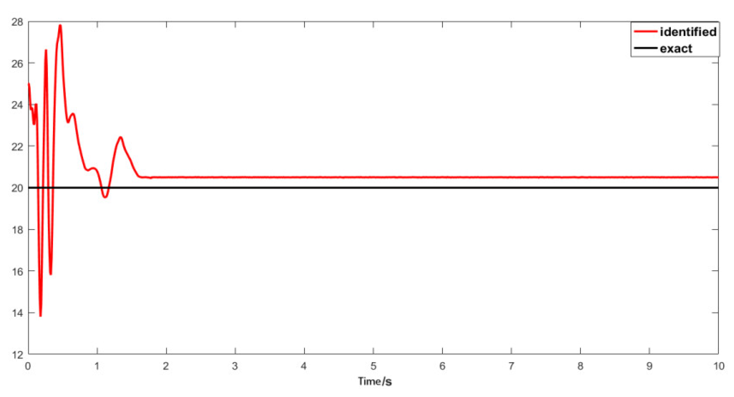
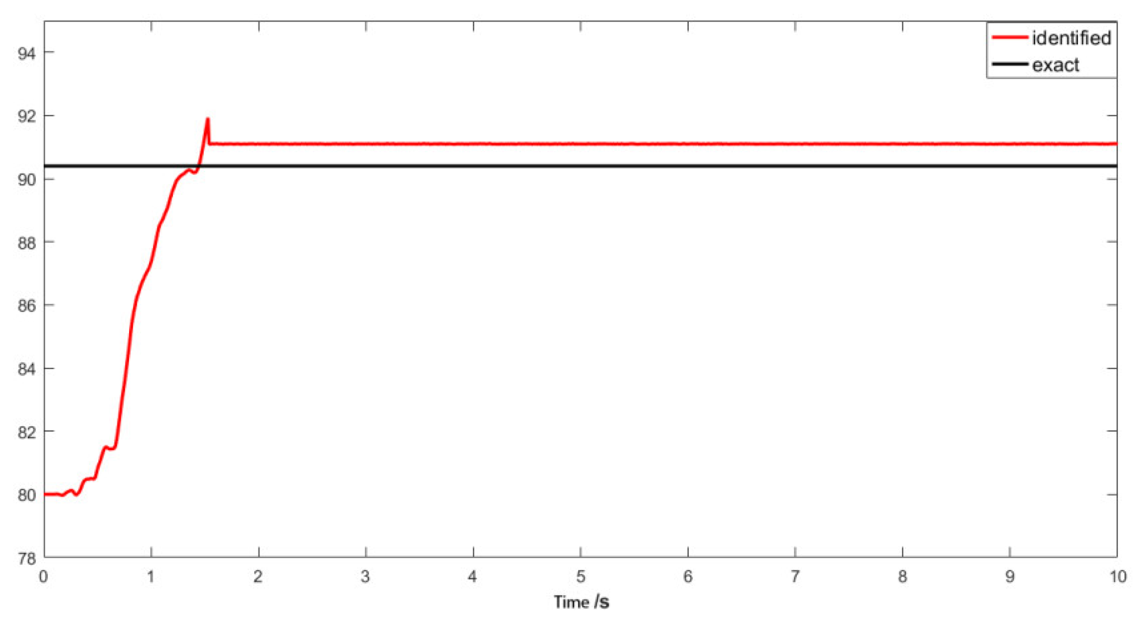
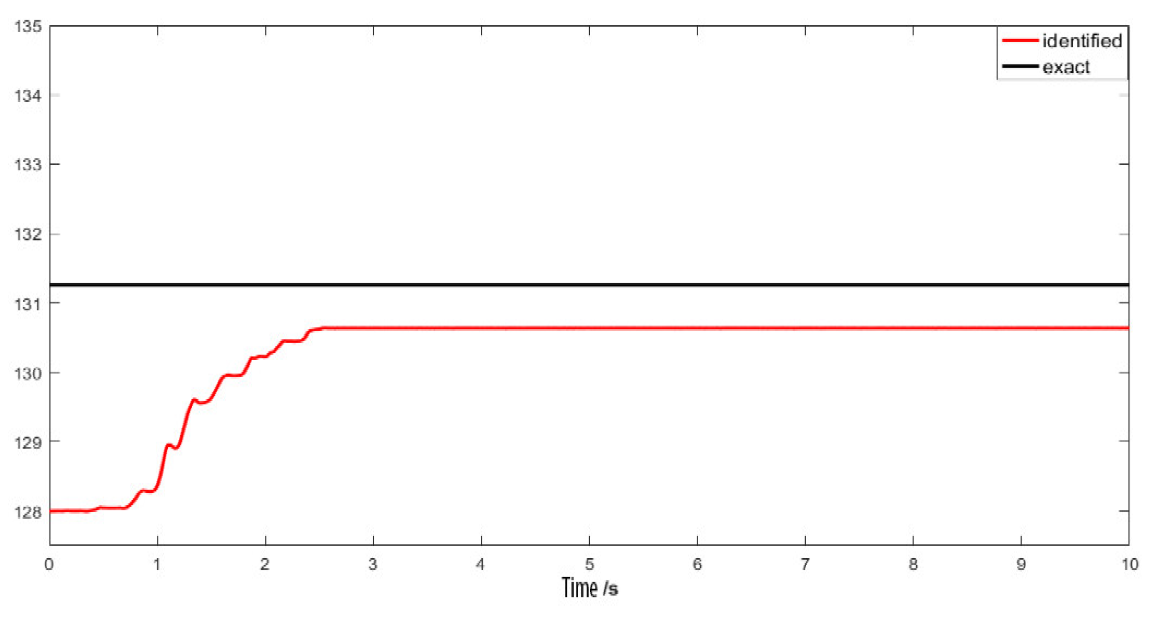
Computational acceleration response data were collected for 10 s, and the sampling interval was 0.01 s. The results showed that the first three natural frequencies of the multi-degree-of-freedom system were $f_1=0.712 \mathrm{H}\mathrm{z}$, $f_2=1.513 \mathrm{H}\mathrm{z}$, and $f_3=1.823 \mathrm{H}\mathrm{z}$. The corresponding generalized stiffness matrix was $\Lambda =\mathrm{d}\mathrm{i}\mathrm{a}\mathrm{g}({\omega }_1^2 {\omega }_2^2 {\omega }_3^2)=\mathrm{d}\mathrm{i}\mathrm{a}\mathrm{g}(20 90.4 131.3)$. The normalized mode shapes of the mass were $\Phi =[{\phi }_1 {\phi }_2 {\phi }_3]$, ${\phi }_1={[0.309 0.413 0.206]}^T$, ${\phi }_2={[0.349 0.056 -0.498]}^T$, and ${\phi }_3={[0.531 -0.277 0.207]}^T$. The excitation position matrix was ${{\rm B}}_f={[0 1 0]}^T$. We considered 25%, 11%, and 5% errors to be applied to the eigenvalues of the generalized stiffness matrix. Thus, the generalized stiffness matrix was given as ${\Lambda }^{\prime }=\mathrm{d}\mathrm{i}\mathrm{a}\mathrm{g}(25 80 128)$. The acceleration responses of the three degrees of freedom were measured. To further test the robustness of the algorithm, the acceleration responses were contaminated with a zero-mean white Gaussian noise with the noise-to-signal ratio being 5%. The parameters to be identified are as follows:

(1)

Augmented state vector $x={\left[q_1 q_2 q_3 {\dot{q}}_1 {\dot{q}}_2 {\dot{q}}_3 {\lambda }_1 {\lambda }_2 {\lambda }_3\right]}^T$;

(2)

Unknown excitation signal.

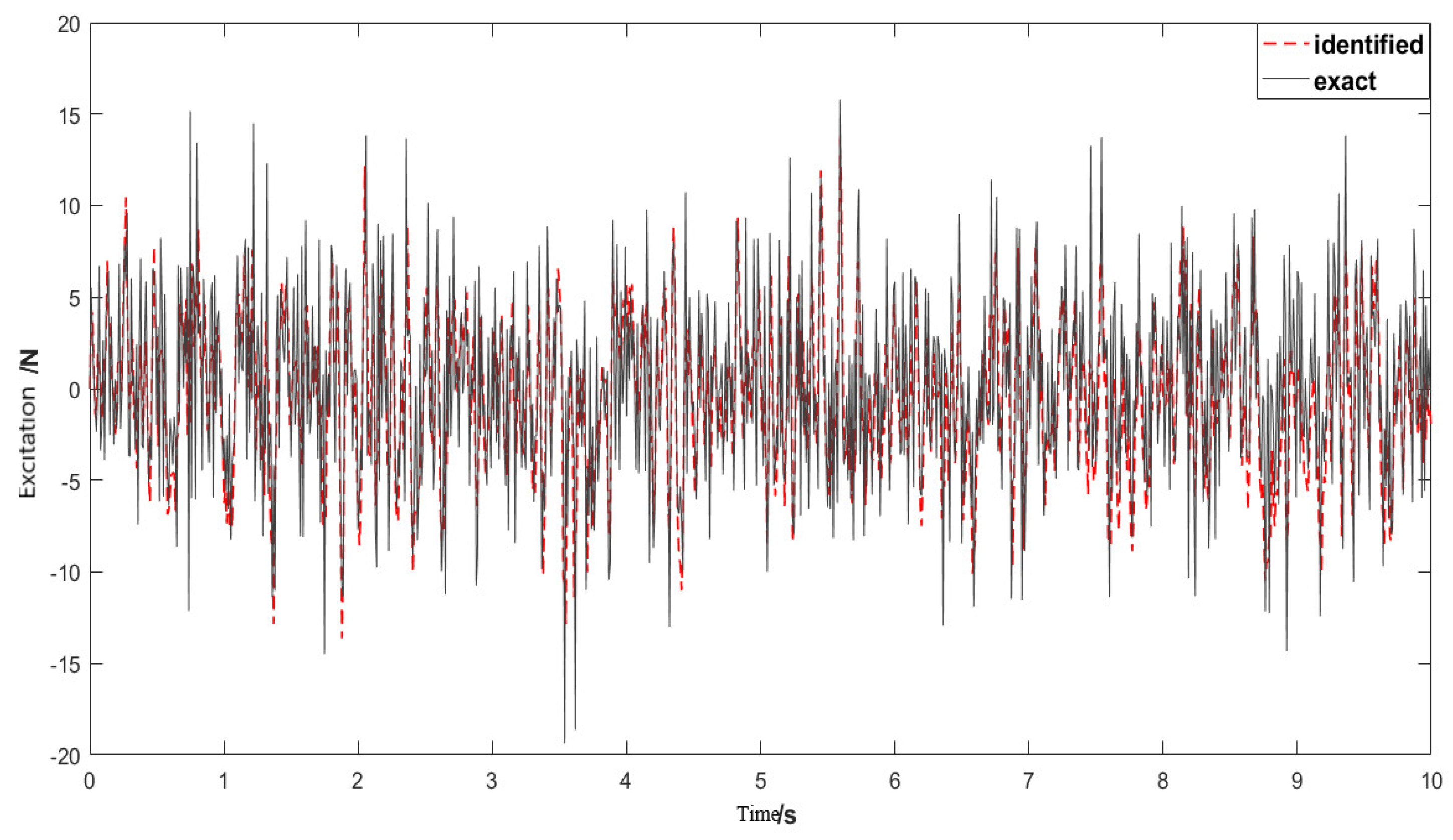
The initial value of the augmented state vector was set to $x_{0|0}={\left[\begin{array}{ccccccccc}0& 0& 0& 0& 0& 0& 25& 80& 128\end{array}\right]}^T$. The initial state prediction covariance was set to $P{x}_{0|0}=\mathrm{d}\mathrm{i}\mathrm{a}\mathrm{g}{[1 1 1 1 1 1 {10}^8 {10}^8 {10}^8]}^T$. The initial value of the excitation was zero. The measured noise covariance and the model noise covariance were set to $R_k={10}^2{{\rm I}}_2$, $G_k={10}^{-1}{{\rm I}}_9$, respectively, where ${{\rm I}}_m$ is the unit matrix. The identification results of the modal parameters and excitation are shown in Figure 2, Figure 3, Figure 4, Figure 5, Figure 6 and Figure 7.

The results in Figure 2, Figure 3 and Figure 4 showed that the modal parameters converged to stable values after several iterations and the recognition accuracy was high. The identification results of the modal parameters and their errors are shown in

Table 3. Modification results of the modal parameters.

Modal Parameter	Convergent Value	Accurate Value	Error (%)
Characteristic value ${\lambda }_1$	20.6	20	3
Characteristic value ${\lambda }_2$	90.6	90.4	0.2
Characteristic value ${\lambda }_3$	130.6	131.26	−0.7
Modal frequency $f_1$(Hz)	0.722	0.712	1.4
Modal frequency $f_2$(Hz)	1.514	1.513	0.06
Modal frequency $f_3$(Hz)	1.818	1.823	-0.2

, where the identified eigenvalues were converted into natural frequencies and compared to the exact values.

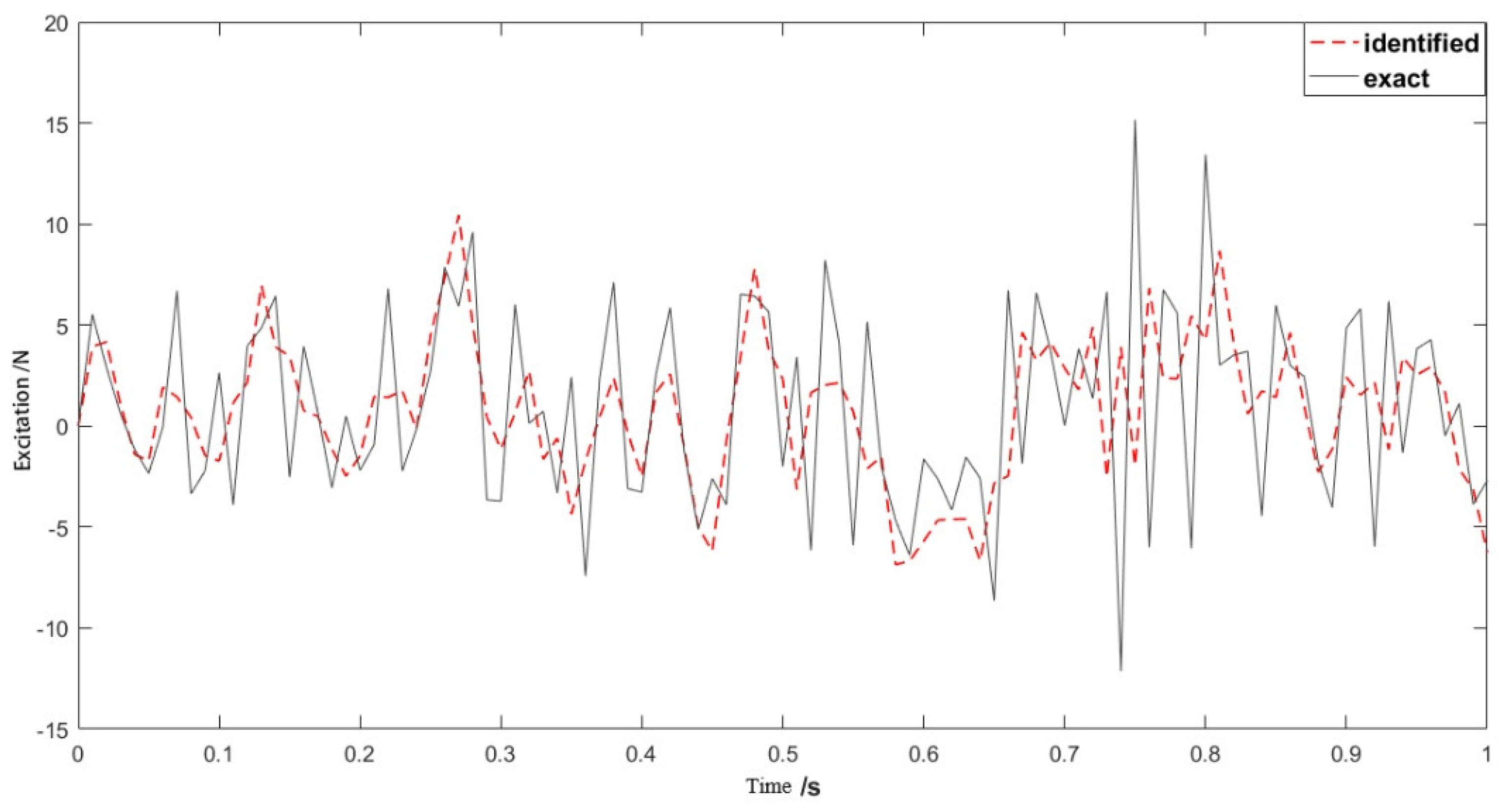
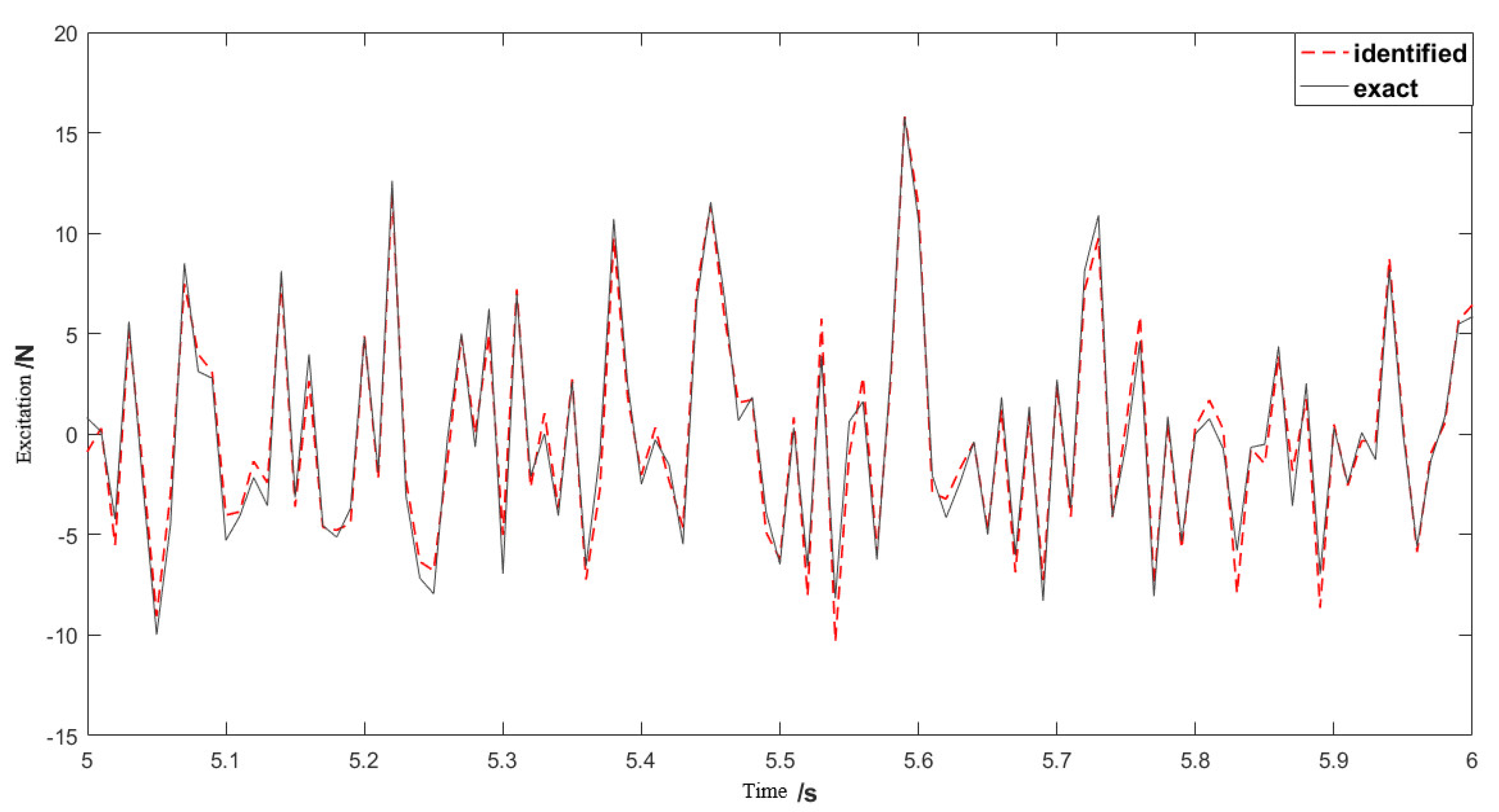
Figure 5, Figure 6 and Figure 7 show the load identification results. It can be seen that the error of the load identification was relatively large in Figure 6. However, the accuracy of the results improved significantly, as the time progresses after the model parameters converged as can be seen in Figure 7. Clearly, the accuracy of the model is dependent on the modal parameters, and once they converge, the load can be identified with good accuracy.

Moreover, to evaluate the accuracy of the identified results, the mean square error (MSE) and the peak relative error method (PREM) were used. The equations to evaluate these errors are shown as follows:

$$MSE(X,Y)={\displaystyle \sum _{i=1}^N{[Y(i)-X(i)]}^2}/N,$$

$$PREM(X,Y)=\left|\frac{\max Y(i)-\max X(i)}{\max X(i)}\right|\times 100\%.$$

Load identification errors for different periods are shown in

Table 4. Error assessment of load identification results in different periods.

Time	MSE	PREM
0–1 s	8.7	93.4
5–6 s	0.056	18.57

. The identified load matched the applied load with good accuracy, despite the noise in the measurements and the initially large errors in the identified modal parameters. Furthermore, the converged modal parameters remained to have some errors and the extended Kalman filter algorithm itself involves a truncation error resulting from considering a finite number of terms in the Taylor expansion. However, the proposed algorithm shows good stability and reliability for modal parameter identification as well as load identification.

4. Experimental Study

In this section, we aimed to evaluate the accuracy of the proposed algorithm using experimental validation. Many engineering metal structures can be abstracted into beams and plates. To this end, a simply supported beam made of steel was used. The acceleration responses of the beam under random loads were collected, and the modal parameters were obtained using the Bayesian modal parameter identification method. Furthermore, the extended Kalman filter in the modal space was used to correct the error parameters and to identify random loads.

The known parameters included the acceleration response of the simply supported beam under a random excitation (generated by a modal shaker) and the mass matrix of the beam. The geometric dimensions and the material properties are shown in

Table 5. Geometric dimensions and material properties of the simply supported beam.

Parameters	Value
length	$a=0.7 \mathrm{m}$
Section width	$b=0.04 \mathrm{m}$
Section height	$h=0.008 \mathrm{m}$
Density	$\rho =7900 \mathrm{k}\mathrm{g}/{\mathrm{m}}^3$
Modulus of elasticity	$E=206 \mathrm{G}\mathrm{P}\mathrm{a}$
Poisson ratio	$\mu =0.3$

.

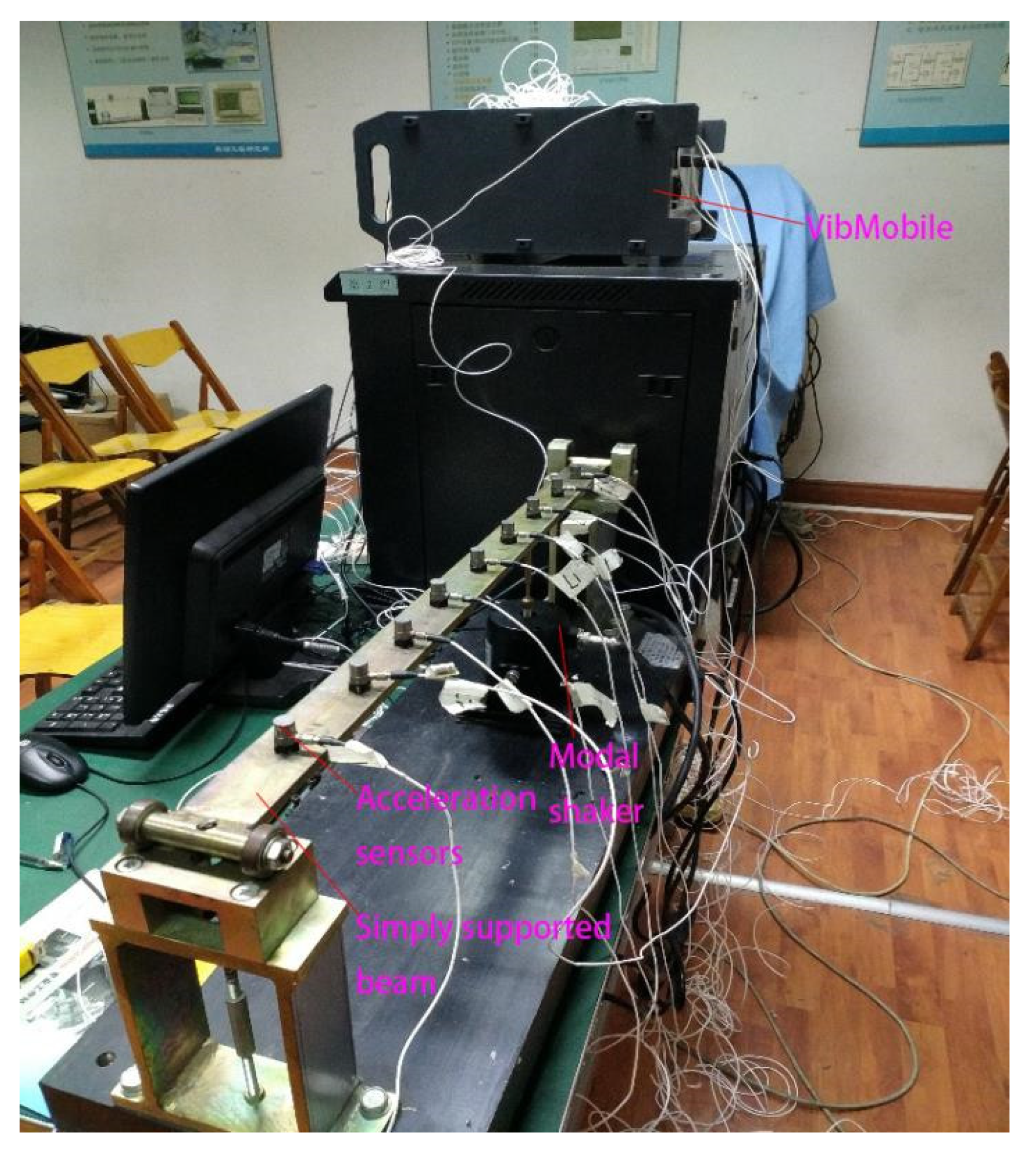
The simply supported beam was meshed into 10 elements, each of which had a length of 0.07 m and a total of 11 nodes. The beam was supported in the vertical direction at the nodes of both ends. The acceleration sensors were placed at the other nine sections. The test setup is shown in Figure 8.

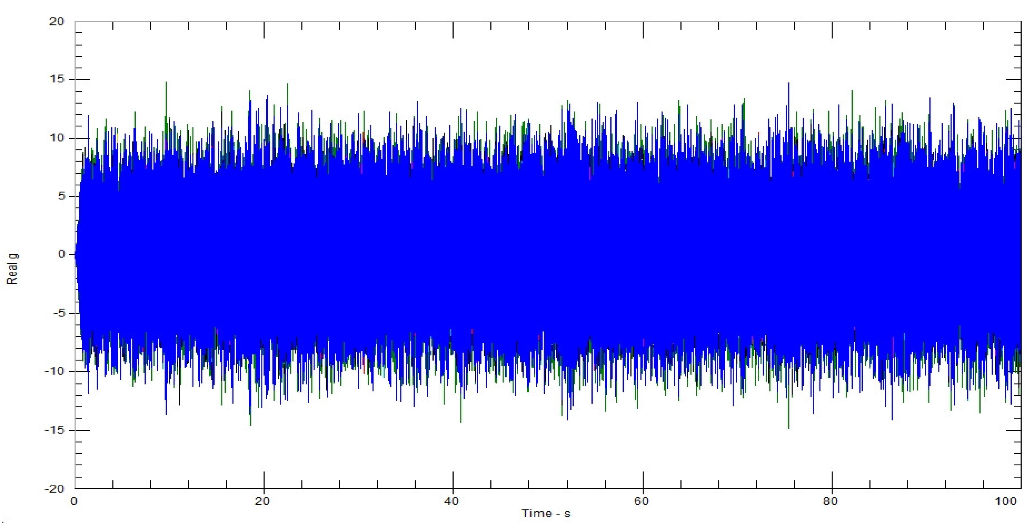
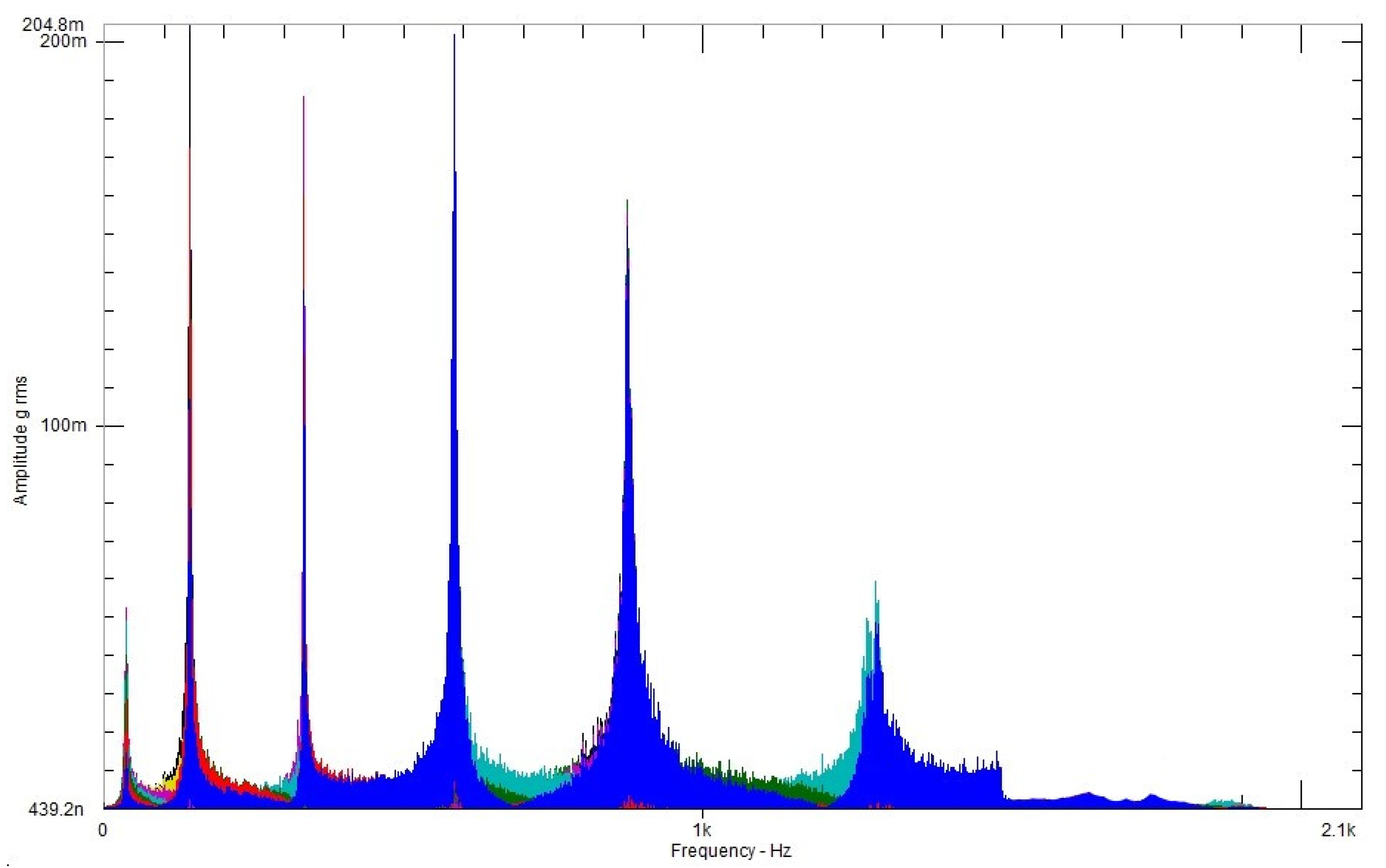
A random excitation with a frequency bandwidth from 0 to 1500 Hz was then applied on the beam. The sampling frequency of the sensor was 4096 Hz. The Fourier transformation of the response signal is shown in Figure 9. Figure 10 shows the Fourier spectra of the response signals.

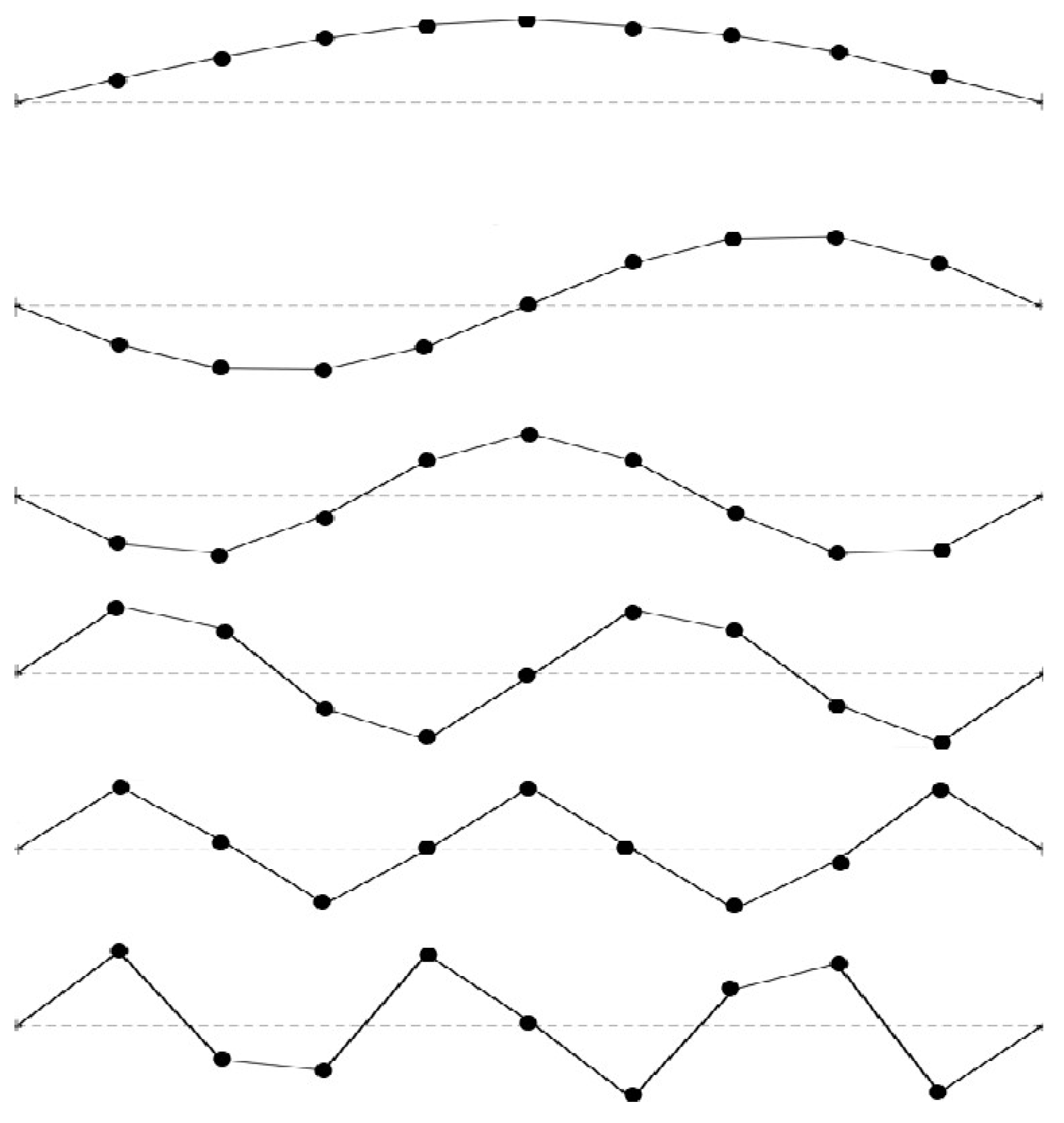
It can be clearly seen that the spectrum had six peaks and the adjacent peaks were far apart. Hence, a single mode analysis can be performed. Furthermore, the seventh mode frequency was 1821 Hz, which was not considered in the simulation. We then considered the frequency corresponding to each peak as an initial value of the modal frequency in the unconstrained numerical optimization equation, which is also called a priori parameter in the Bayesian theory. The initial assumptions and the frequency bands are shown in

Table 6. Initial assumptions and initial frequency bands.

Mode	Initial Assumption (Hz)	Frequency Band (Hz)
		Lower	Upper
1	39	38	40
2	150.1	145	155
3	339.2	330	350
4	602.6	590	615
5	931.8	900	960
6	1322.6	1290	1360

. The identified modes are shown in Figure 11.

Four frequency bands were selected for each order modal analysis. The final modal frequency and damping ratio were the average values of the four calculations.

Table 7. Identification results of the modal parameters.

Modal	Modal Frequency MPV(Hz)		Damping Ratio MPV (%)		MAC
	Identification Value	Test Value	Identification Value	Test Value
1	38.12	38.14	0.88	1.08	1
2	149.1	149.13	0.42	0.31	0.997
3	336.4	336.36	0.16	0.21	1
4	597.6	594.73	0.23	0.24	1
5	928.8	920.23	1.04	1.16	0.995
6	1314.2	1300.29	0.8	0.48	0.99

shows the identification values of the modal frequencies and the damping ratios for each order of the modal analysis compared with the results of the modal tests, as well as the MAC values of each mode.

The results shown in Table 7 indicated that the Bayesian modal parameter identification method has relatively large errors in the identification of high-order modal frequencies. Hence, the first two modal frequencies can be considered to be accurate. The third to sixth order modal frequencies were used as errors parameters to form an extended vector with the state vector. The extended Kalman filter load identification method in the modal space was then used to correct these errors parameters and to identify the time-domain load.

The modal error parameter vector was $\theta =\left[\begin{array}{cccc}{\lambda }_3& {\lambda }_4& {\lambda }_5& {\lambda }_6\end{array}\right]$. The extended state vector was then $x=\left[\begin{array}{ccc}{q}_1& q_2& \begin{array}{ccc}\cdots & q_6& \begin{array}{ccc}{\dot{q}}_1& {\dot{q}}_2& \cdots \begin{array}{ccc}{\dot{q}}_6& {\lambda }_3& \begin{array}{cc}{\lambda }_4& \begin{array}{cc}{\lambda }_5& {\lambda }_6\end{array}\end{array}\end{array}\end{array}\end{array}\end{array}\right]$. The unknown quantities to be identified are as follows:

• The extended vector;
• The random excitation.

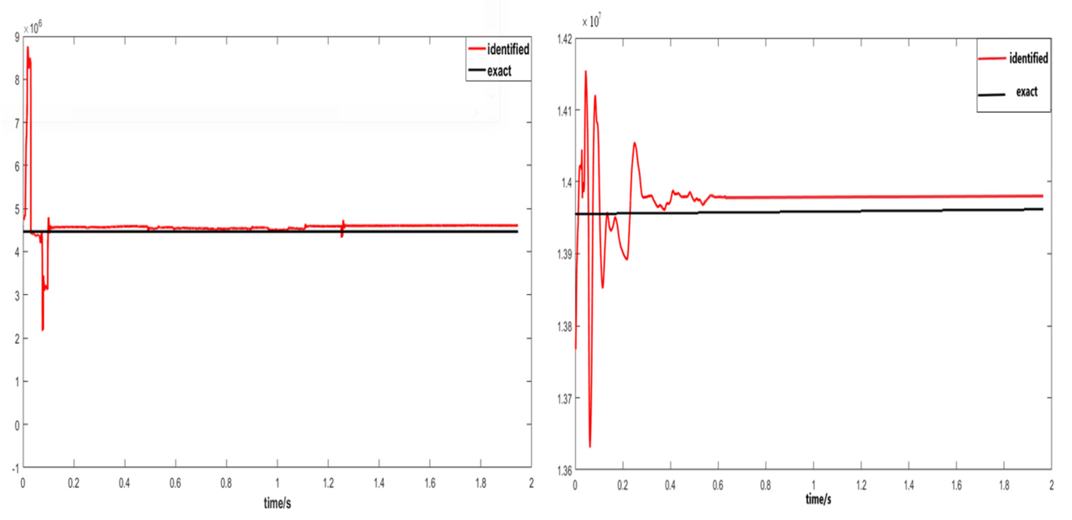
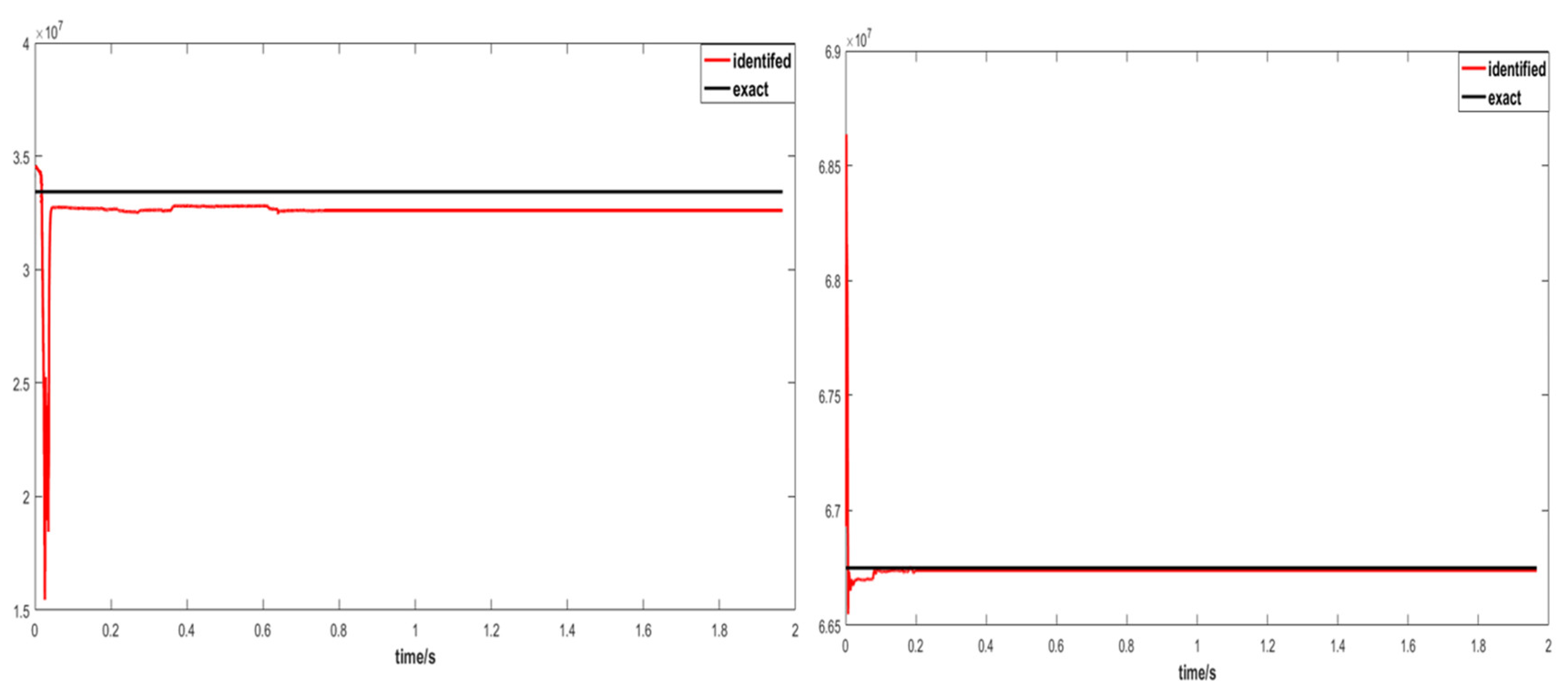
The initial values for the state variables were zero, and the initial assumptions for ${\lambda }_3,{\lambda }_4,{\lambda }_5,{\lambda }_6$ were the identified values: ${\lambda }_i={\left(2\pi f_i\right)}^2$. The initial error covariance matrix of the extended state vector was taken to be $P{x}_{0|0}=diag[1{ 1 1 1 1 1 1 1 1 1 1 1 10}^8{ 10}^8{ 10}^{10}]$. The initial value of the excitation was zero. The covariance matrices of both the measurement noise and the model noise were chosen to be $R_k={10}^2{I}_6$ and $G_k=I_{18}$, respectively. The identified parameters are presented in Figure 12 and Figure 13. The identified eigenvalues and the natural frequencies and the error comparisons are shown in the

Table 8. Eigenvalue and modal frequency identification results.

Modal Parameters	${\mathit{\lambda }}_3$	${\mathit{\lambda }}_4$	${\mathit{\lambda }}_5$	${\mathit{\lambda }}_6$	${\mathit{f}}_3\left(\mathbf{Hz}\right)$	${\mathit{f}}_4\left(\mathbf{Hz}\right)$	${\mathit{f}}_5\left(\mathbf{Hz}\right)$	${\mathit{f}}_6\left(\mathbf{Hz}\right)$
Identification value	4.48 × 106	1.39 × 107	3.29 × 107	6.67 × 107	336.96	595.07	914.52	1299.91
Test value	4.46 × 106	1.39 × 107	3.34 × 107	6.67 × 107	336.36	594.73	920.23	1300.29
Error (%)	2.57	0.14	−2.66	−0.06	0.17	0.057	−0.65	−0.15

. In the first few iterations of filtering, the identified value had a very large jump, but it converged to the exact value after several iterations.

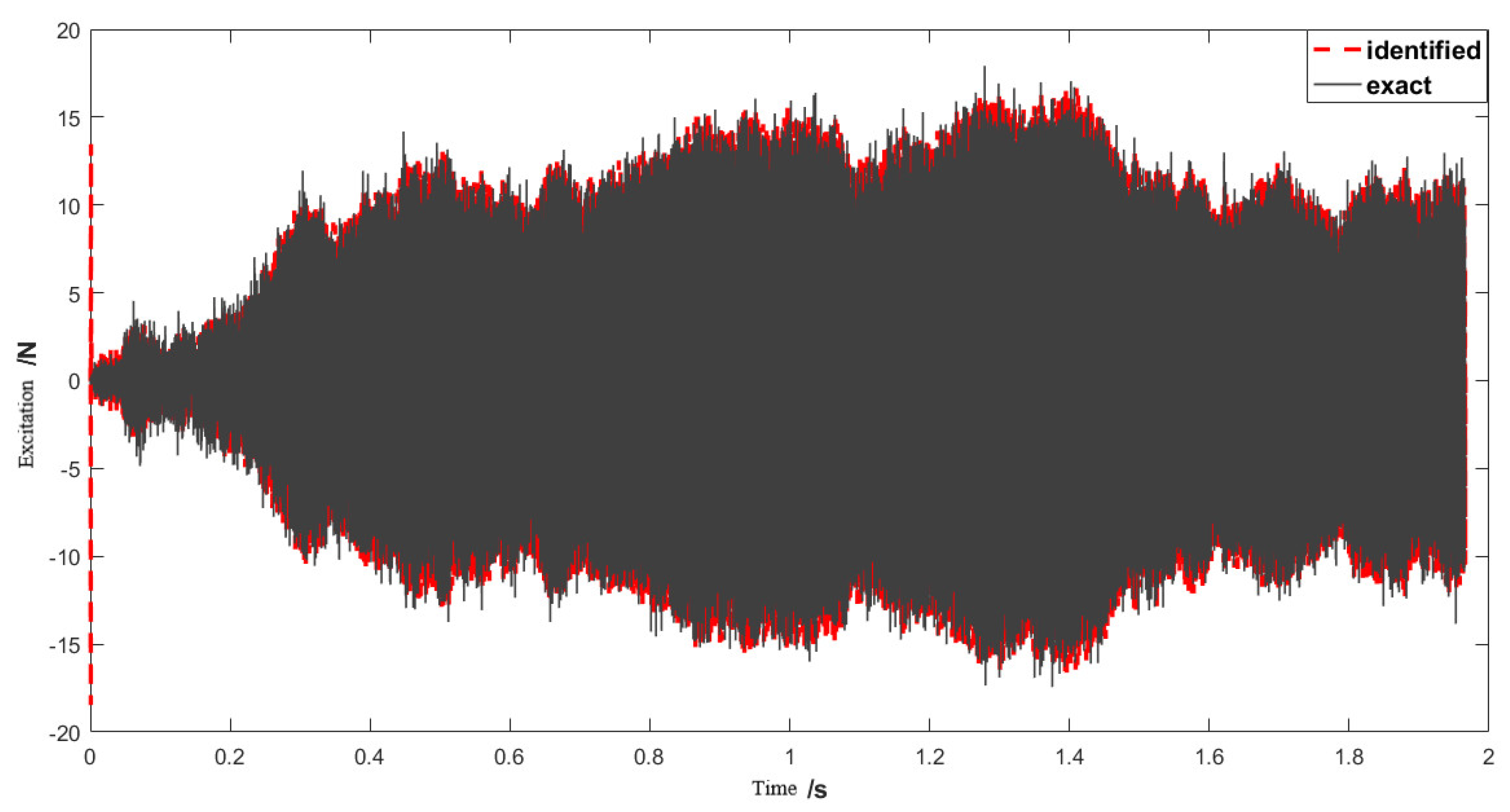
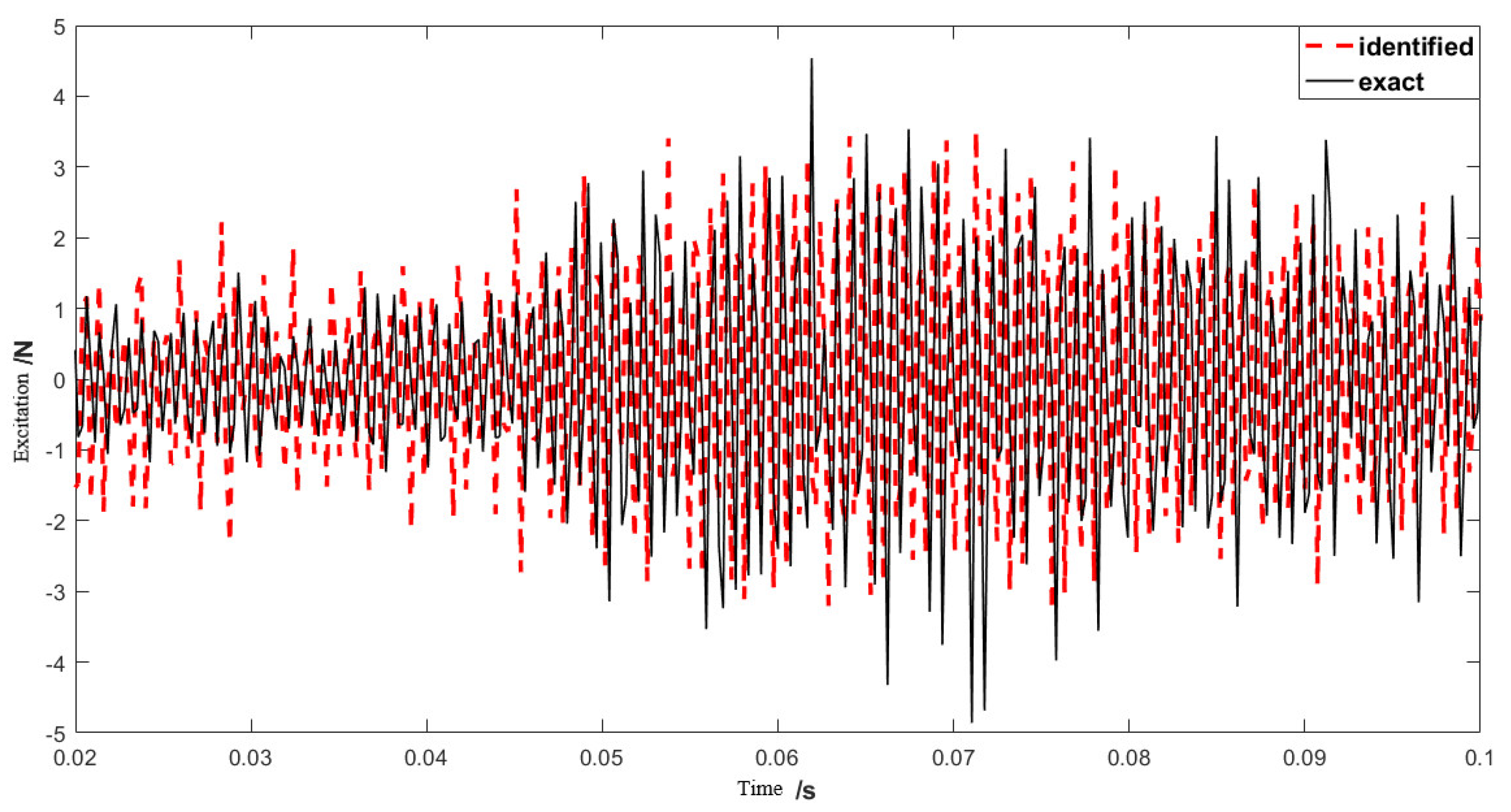
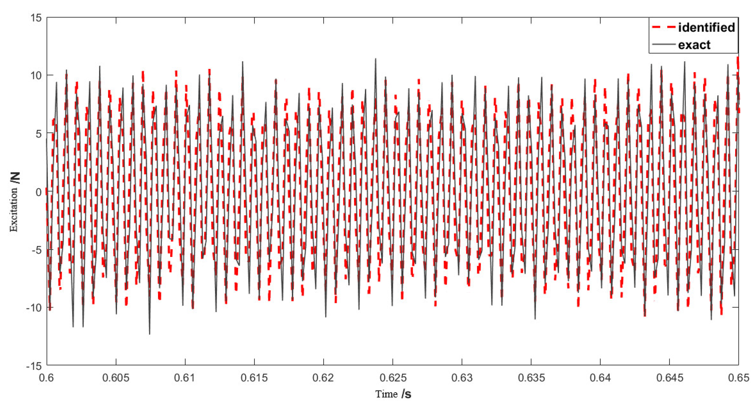
Figure 14 shows the identified load for the first two seconds. Since the identification result was extremely abnormal in several iterative steps of the initial calculation, the statistics started from 0.02 s. Figure 15 shows the load from 0.02 to 0.1 s when the parameters were still being identified. Figure 16 shows the excitation identification results from 0.6 to 0.65 s, during which the modal parameters converged.

The MSE and the PREM were evaluated for the time span from 0.02 to 0.1 s, where the identification algorithm is still in the process of the model parameters updating. The errors measurements were then evaluated again for the time span from 0.6 to 0.65 s, when the load identification started to use converged parameters. The errors for both time spans are displayed in

Table 9. Statistical errors of load identification results in different periods.

Periods (s)	MSE	PREM
0.02–0.5	3.6	174.4
0.6–0.65	1.34	26.7

. The errors showed a significant improvement in the error once the algorithm has converged. The small errors for the time span from 0.6 to 0.65 s showed a good accuracy of the proposed algorithm in capturing the dynamic load.

5. Conclusions

In this paper, we proposed an algorithm for identifying the modal parameters and the dynamic load of an unspecified metal system using the system measured response. We used the Bayesian FFT to identify the modal parameters under the ambient excitation. Hence, the prior parameters of the modal frequency were obtained from the FFT spectrum of the measured response. Then, the modal parameters were refined using numerical unconstrained optimization. It should be noted that the resonance frequency band needs to be selected manually. The dynamic load identification method based on the extended Kalman filter was firstly derived in the modal space.

The results obtained from the numerical test of a 3-DOFs system and then an experiment of a random load applied on a simply supported steel beam demonstrated the advantages of the proposed method in identifying the applied dynamic loads. The main conclusions are as follows:

(1)

The modal parameters identified by the single-mode identification method had good accuracy. They were the initial values of the subsequent algorithm and can be further improved by iteration.

(2)

At the initial stage of load identification, the modal parameters were still in the progress of revision and did not converged. As a result, the error of the load was large. After many iterations, the error modal parameters converged to a stable value, and the recognition accuracy of the load was high.

(3)

The algorithm is suitable for large-scale structures with discrete model errors. It can reduce the amount of calculation while ensuring the calculation accuracy in the modal space compared with the methods in the time domain. It is simple, reliable and easy to be coded.

References

1. Bai, X.; Wei, X.; Ma, Q.; An, Z. Failure Rate Model of Materials under Uncertain Constant Amplitude Cyclic Load. Metals 2022, 12, 1181. [Google Scholar] [CrossRef]
2. Wang, L.; Peng, Y.; Xie, Y.; Chen, B.; Du, Y. A new iteration regularization method for dynamic load identification of stochastic structures. Mech. Syst. Signal Process. 2021, 156, 107586. [Google Scholar] [CrossRef]
3. Liu, R.; Dobriban, E.; Hou, Z.; Qian, K. Dynamic Load Identification for Mechanical Systems: A Review. Arch. Comput. Methods Eng. 2022, 29, 831–863. [Google Scholar] [CrossRef]
4. Li, H.; Jiang, J.; Mohamed, M. Online Dynamic Load Identification Based on Extended Kalman Filter for Structures with Varying Parameters. Symmetry 2021, 13, 1372. [Google Scholar] [CrossRef]
5. Jiang, J.; Ding, M.; Li, J. A novel time-domain dynamic load identification numerical algorithm for continuous systems. Mech. Syst. Signal Process. 2021, 160, 107881. [Google Scholar] [CrossRef]
6. Yang, H.; Jiang, J.; Chen, G.; Mohamed, M.S.; Lu, F. A Recurrent Neural Network-Based Method for Dynamic Load Identification of Beam Structures. Materials 2021, 14, 7846. [Google Scholar] [CrossRef]
7. Yang, H.; Jiang, J.; Chen, G.; Zhao, J. Dynamic load identification based on deep convolution neural network. Mech. Syst. Signal Process. 2023, 185, 109757. [Google Scholar] [CrossRef]
8. Ronasi, H.; Johansson, H.; Larsson, F. A numerical framework for load identification and regularization with application to rolling disc problem. Comput. Struct. 2011, 89, 38–47. [Google Scholar] [CrossRef]
9. Pan, C.D.; Yu, L.; Liu, H.L. Identification of moving vehicle forces on bridge structures via moving average Tikhonov regularization. Smart Mater. Struct. 2017, 26, 085041. [Google Scholar] [CrossRef]
10. Huang, F.-L.; Wang, X.-M.; Chen, Z.-Q.; He, X.-H.; Ni, Y.-Q. A new approach to identification of structural damping ratios. J. Sound Vib. 2007, 303, 144–153. [Google Scholar] [CrossRef]
11. Mirtaheri, M.; Salehi, F. Ambient vibration testing of existing buildings: Experimental, numerical and code provisions. Adv. Mech. Eng. 2018, 10, 1687814018772718. [Google Scholar] [CrossRef] [Green Version]
12. Ibrahim, S.R. An upper hessenberg sparse matrix algorithm for modal identification on minicomputers. J. Sound Vib. 1987, 113, 47–57. [Google Scholar] [CrossRef]
13. Lardies, J.; Larbi, N. A new method for model order selection and modal parameter estimation in time domain. J. Sound Vib. 2001, 245, 187–203. [Google Scholar] [CrossRef]
14. Liu, K. Modal parameter estimation using the state space method. J. Sound Vib. 1996, 197, 387–402. [Google Scholar] [CrossRef]
15. Yuen, K.-V.; Katafygiotis, L.S.; Beck, J.L. Spectral density estimation of stochastic vector processes. Probabilistic Eng. Mech. 2002, 17, 265–272. [Google Scholar] [CrossRef]
16. Yuen, K.-V.; Katafygiotis, L.S. Bayesian Fast Fourier Transform Approach for Modal Updating Using Ambient Data. Adv. Struct. Eng. 2003, 6, 81–95. [Google Scholar] [CrossRef]
17. Feng, W.; Li, Q.; Lu, Q.; Li, C.; Wang, B. Element-wise Bayesian regularization for fast and adaptive force reconstruction. J. Sound Vib. 2020, 490, 115713. [Google Scholar] [CrossRef]
18. De Freitas, J.F.G.; Niranjan, M.; Gee, A.H.; Doucet, A. Sequential Monte Carlo Methods to Train Neural Network Models. Neural Comput. 2014, 12, 955–993. [Google Scholar] [CrossRef]
19. Azam, S.E.; Chatzi, E.; Papadimitriou, C. A dual Kalman filter approach for state estimation via output-only acceleration measurements. Mech. Syst. Signal Process. 2015, 60–61, 866–886. [Google Scholar] [CrossRef]
20. Lei, Y.; Jiang, Y.; Xu, Z. Structural damage detection with limited input and output measurement signals. Mech. Syst. Signal Process. 2012, 28, 229–243. [Google Scholar] [CrossRef]
21. Zhang, E.; Antoni, J.; Feissel, P. Bayesian force reconstruction with an uncertain modal. J. Sound Vib. 2012, 331, 798–814. [Google Scholar] [CrossRef]
22. Yan, G. A Bayesian approach for impact load identification of stiffened composite panel. Inverse Probl. Sci. Eng. 2014, 22, 940–965. [Google Scholar] [CrossRef]
23. Faure, C.; Ablitzer, F.; Antoni, J.; Pézerat, C. Empirical and fully Bayesian approaches for the identification of vibration sources from transverse displacement measurements. Mech. Syst. Signal Process. 2017, 94, 180–201. [Google Scholar] [CrossRef]
24. Hwang, J.S.; Lee, S.G.; Ji-hoon, P.; Eun-Jong, Y. Force identification from structural responses using kalman filter. Inst. Mater. Eng. 2008, 33, 257–266. [Google Scholar]
25. Lourens, E.; Reynders, E.; De Roeck, G.; Degrande, G.; Lombaert, G. An augmented Kalman filter for force identification in structural dynamics. Mech. Syst. Signal Process. 2012, 27, 446–460. [Google Scholar] [CrossRef]
26. Naets, F.; Cuadrado, J.; Desmet, W. Stable force identification in structural dynamics using Kalman filtering and dummy-measurements. Mech. Syst. Signal Process. 2015, 50–51, 235–248. [Google Scholar] [CrossRef]
27. Yang, J.N.; Pan, S.; Lin, S. Least-Squares Estimation with Unknown Excitations for Damage Identification of Structures. J. Eng. Mech. 2007, 133, 12–21. [Google Scholar] [CrossRef]
28. Yang, J.N.; Lin, S.; Huang, H.W.; Zhou, L. An adaptive extended Kalman filter for structural damage identification. Struct. Control Health Monit. 2006, 13, 849–867. [Google Scholar] [CrossRef]
29. Yang, J.N.; Pan, S.; Huang, H.-W. An adaptive extended Kalman filter for structural damage identifications II: Unknown inputs. Struct. Control Health Monit. 2007, 14, 497–521. [Google Scholar] [CrossRef]
30. Débarbouillé, A.; Renaud, F.; Dimitrijevic, Z.; Chojnacki, D.; Rota, L.; Dion, J.-L. Wheel forces estimation with an Augmented and Constrained Extended Kalman Filter applied on a nonlinear multi-body model of a half vehicle. Procedia Struct. Integr. 2022, 38, 342–351. [Google Scholar] [CrossRef]
31. Ding, Y.; Zhao, B.; Wu, B.; Zhang, X.; Guo, L. Simultaneous identification of structural parameter and external excitation with an improved unscented kalman filter. Adv. Struct. Eng. 2015, 11, 5–18. [Google Scholar] [CrossRef]
32. Wang, B.P. Improved Approximate Methods for Computing Eigenvector Derivatives in Structural Dynamics. AIAA J. 1991, 29, 1018–1020. [Google Scholar] [CrossRef]
Figure 1. DOF structure.
Metals 12 01872 g001
Figure 2. λ 1 Identification result diagram.
Metals 12 01872 g002
Figure 3. λ 2 Identification result diagram.
Metals 12 01872 g003
Figure 4. λ 3 Identification result diagram.
Metals 12 01872 g004
Figure 5. Load identification results.
Metals 12 01872 g005
Figure 6. Load identification results from 0–1 s.
Metals 12 01872 g006
Figure 7. Load identification results from 5–6 s.
Metals 12 01872 g007
Figure 8. Test setup.
Metals 12 01872 g008
Figure 9. Acceleration response signals of all channels.
Metals 12 01872 g009
Figure 10. Fourier spectra of the response signals.
Metals 12 01872 g010
Figure 11. Identification of the first six modes.
Metals 12 01872 g011
Figure 12. Identified parameters of λ 3 and λ 4 .
Metals 12 01872 g012
Figure 13. Identified parameters of λ 5 and λ 6 .
Metals 12 01872 g013
Figure 14. Identified excitation from 0 to 2 s.
Metals 12 01872 g014
Figure 15. Identified excitation from 0.02 to 0.1 s.
Metals 12 01872 g015
Figure 16. Identified excitation from 0.6 to 0.65 s.
Metals 12 01872 g016