Computational Pipeline for Glomerular Segmentation and Association of the Quantified Regions with Prognosis of Kidney Function in IgA Nephropathy

Abstract

The histopathological findings of the glomeruli from whole slide images (WSIs) of a renal biopsy play an important role in diagnosing and grading kidney disease. This study aimed to develop an automated computational pipeline to detect glomeruli and to segment the histopathological regions inside of the glomerulus in a WSI. In order to assess the significance of this pipeline, we conducted a multivariate regression analysis to determine whether the quantified regions were associated with the prognosis of kidney function in 46 cases of immunoglobulin A nephropathy (IgAN). The developed pipelines showed a mean intersection over union (IoU) of 0.670 and 0.693 for five classes (i.e., background, Bowman’s space, glomerular tuft, crescentic, and sclerotic regions) against the WSI of its facility, and 0.678 and 0.609 against the WSI of the external facility. The multivariate analysis revealed that the predicted sclerotic regions, even those that were predicted by the external model, had a significant negative impact on the slope of the estimated glomerular filtration rate after biopsy. This is the first study to demonstrate that the quantified sclerotic regions that are predicted by an automated computational pipeline for the segmentation of the histopathological glomerular components on WSIs impact the prognosis of kidney function in patients with IgAN.

1. Introduction

The number of patients who are on dialysis due to end-stage renal failure is increasing worldwide, which has become a major health economic problem. According to a recent report [1], the number of patients undergoing chronic dialysis worldwide exceeded two million in 2010, and this number may double by 2030. The early detection and management of chronic kidney disease (CKD) is important in order to prevent its progression to end-stage renal failure. Immunoglobulin A nephropathy (IgAN) is the leading cause of CKD worldwide. It typically progresses to end-stage renal failure in 15–20% of patients after 10 years, and approximately 40% of patients after around 20 years [2,3]. Using evidence-based clinical practice guidelines in Japan [4], the clinical predictors for the progression of IgAN at the time of the initial renal biopsy include the following: (1) the presence of hypertension; (2) the amount of proteinuria with a usual cut-off of >1 g/day; (3) the degree of renal dysfunction; and (4) the histopathological grade, based on renal pathology. Of these predictors, histopathological findings play a key role but require observation by experts under a microscope. Patients with IgAN have varied histopathological lesions, ranging from mild mesangial proliferation, endocapillary hypercellularity, and crescentic glomerulonephritis to global and segmental sclerosis. For example, sclerosis represents the final appearance of glomerular injury that is caused by various diseases. When sclerosis occurs globally, determining the cause of the injury can be difficult.

Two histopathological grading systems are referred to in the clinical guidelines. The first system is the Oxford classification [5,6], which is based on the score of mesangial hypercellularity (M: M0, ≤0.5; M1, >0.5), endocapillary hypercellularity (E: E0, absent; E1, present), segmental sclerosis (S: S0, absent; S1, present), tubular atrophy or interstitial fibrosis (T: T0, 0–25%; T1, 26–50%; T2, >50%), and cellular or fibrocellular crescents (C: C0, absent; C1, 0–25%; C2, >25%). The second system is the Japanese histological grade classification (H-Grade) [7,8], which is based on the presence of acute lesions (i.e., cellular crescent, tuft necrosis, and fibrocellular crescent) and chronic lesions (i.e., global sclerosis, segmental sclerosis, and fibrous crescent). Detecting these complex findings among all of the glomeruli in whole slide images (WSIs) is laborious and time consuming, even for highly trained pathologists or nephrologists. Furthermore, the assessment is not always consistent [9,10]. Suppose the findings of all of the glomeruli on a WSI could be quantified with a computer, it may lead to a more thorough investigation of their impact on the prognosis of immunoglobulin A nephropathy (IgAN) and accelerate such research.

In the past decade, the number of studies aiming to develop deep learning applications for nephropathology has increased rapidly. Computational image recognition focusing on the glomerulus is generally classified into the following three types: the detection of glomeruli [11,12,13,14], the classification of the glomeruli [10,15], and the segmentation of the glomeruli [16,17,18,19,20,21,22,23,24]. The glomeruli that are detected in the WSI are localized by drawing bounding boxes. This approach would be a good application of automation because detecting glomeruli is simple but tedious for humans. Additionally, the development of such tools is realistic, as previously reported [13]. The classification of glomeruli, such as the presence or the absence of certain pathological findings, is more challenging because it requires the interpretation of quantitative histopathological lesions into qualitative expressions, for which expert assessment is not always consistent [9,10]. The segmentation of glomeruli localizes and quantifies every glomerulus by identifying the regions of each glomerulus in the pixels. Several studies have attempted to distinguish between the entire glomerulus and the background [16,17] or to distinguish between the normal and the sclerotic glomeruli [20,21,24]. Other studies have focused on the tubules, the blood vessels, and the interstitium, in addition to the glomerulus [19,23], or on the components inside of the glomerulus [18,22]. Segmenting the glomerulus and its components would be more helpful for a better understanding of kidney disease because it will be applied in the classification of pathological findings and to develop a prognostic model by utilizing quantified histopathological regions.

Table 1. Previous studies for glomerular segmentation from WSI.

Author	Year	Object	Method	Subsequent Analysis	Extrapolation Evaluation
Kato et al. [16]	2015	Glomerulus	S-HOG + SVM	-	-
Gallego et al. [17]	2018	Glomerulus	CNN	-	-
Ginley et al. [18]	2019	Glomerulus and Internal components ((1) a nuclear component; (2) a PAS-positive component consisting of mesangium, glomerular basement membranes, and Bowman’s capsule; (3) a luminal component consisting of Bowman’s space and capillary lumina)	Deep Lab v2	Tervaert classification and classification scheme defined by authors	-
Hermsen et al. [19]	2019	Renal structures (glomerulus, sclerotic glomerulus, empty Bowman’s capsules, proximal tubule, distal tubule, atrophic tubule, undefined tubule, artery, interstitium, and capsule)	U-Net	Banff classification	Radboud University and Mayo Clinic
Bueno et al. [20]	2020	Glomerulus (normal, sclerosed)	SegNet and U-Net	-	-
Antini et al. [21]	2020	Glomerulus (normal, sclerosed)	SegNet and Deeplab v3+	-	-
Zeng et al. [22]	2020	Glomerulus (global sclerosis, segmental sclerosis, crescent, or none of the above) and intraglomerular structures (mesangial cells, endothelial cells, and podocytes)	U-Net, DenseNet, LSTM-GCNet, and 2D V-Net	Mesangial hypercellularity score	-
Bouteldja et al. [23]	2021	Renal structures (glomerular tuft, glomerulus including Bowman’s capsule, tubules, arteries, arterial lumina, and veins)	U-Net	-	-
Jiang et al. [24]	2021	Glomerulus (normal, global sclerosis, and glomerular with other lesions)	Mask R-CNN	-	-

shows the previous studies for glomerular segmentation from WSI.

As the configuration of segmentation tasks varies from researcher to researcher, the high performance of a machine learning model does not necessarily indicate its usefulness for subsequent analyses. Previous studies [18,19,22] have assessed the usefulness of segmentation results in subsequent analyses, whereas other studies have only assessed the performance of machine learning models. 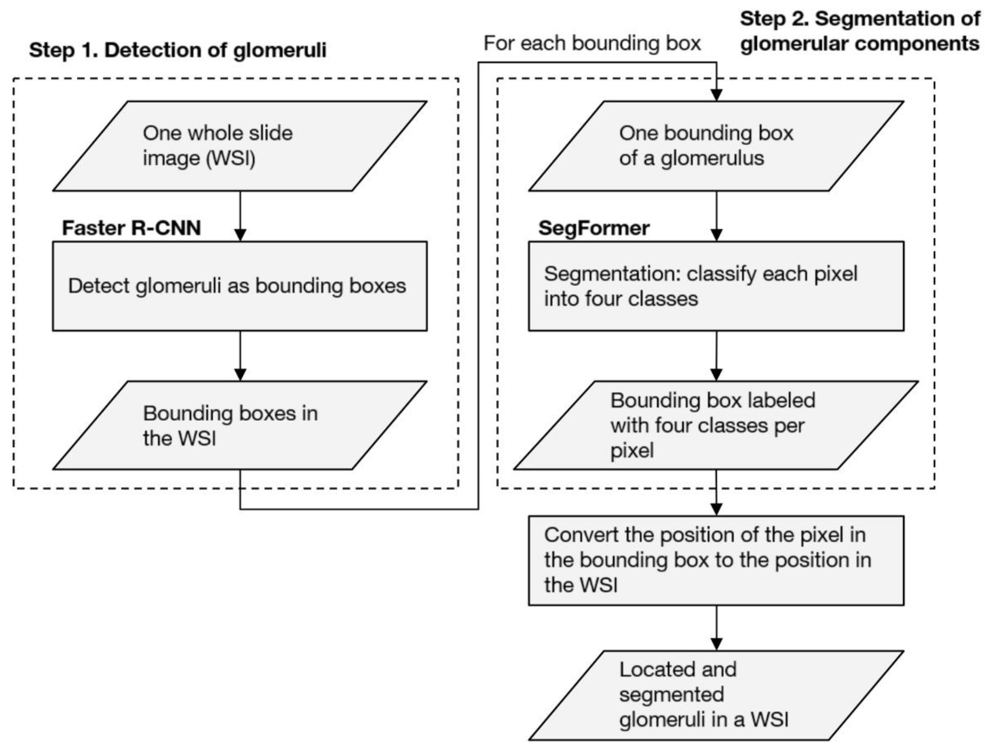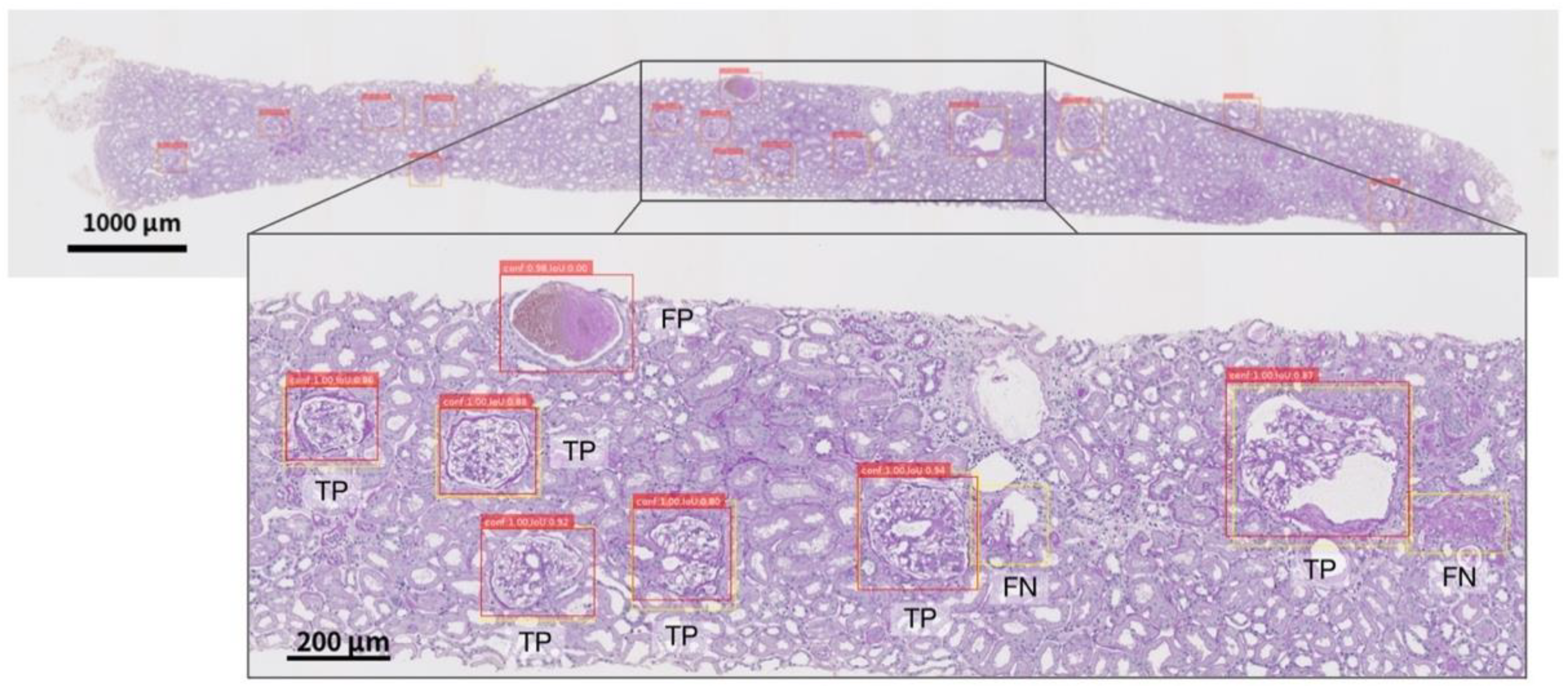In addition, these previous studies have only [19] evaluated the performance of machine learning models against external WSI, whereas the other studies have evaluated a single facility. Due to their high performance, deep neural networks (DNNs) tend to overfit to minute differences in the images that are used for training. Furthermore, the pathological specimens differ between facilities due to the differences in the preparation protocols. These factors have a non-negligible impact on the generalizability of studies dealing with WSI in DNNs. Therefore, in assessing the performance of the developed DNNs, an internal evaluation using only the WSIs of a single facility is not sufficient; external evaluations of the WSIs of different facilities are also important. Based on these two points, we propose an automated computational pipeline to detect the glomeruli from periodic acid-Schiff (PAS)-stained WSI and to segment the Bowman’s space, the glomerular tuft, and the histopathological components of crescentic and sclerotic regions. The pipelines were developed using the WSIs of two facilities independently, and the performances across the facilities were evaluated. In order to assess the significance of the quantified histopathological regions, we conducted a multivariate regression analysis to determine whether the proportion of the sclerotic regions was significantly associated with the prognosis of kidney function in patients with IgAN.

2. Materials and Methods

2.1. Data Collection

The Institutional Review Board approved all experiments and data collection at the University of Tokyo Hospital (Tokyo, Japan; approval number: 11455) and Tazuke Kofukai Medical Research Institute, Kitano Hospital (Osaka, Japan; approval number: P17-05-004). All of the experiments were conducted following the Ethical Guidelines for Medical and Biological Research Involving Human Subjects in Japan. Informed consent was obtained from all participants through opt-out on the website. (See Figure A1 in Appendix A for an overview of the data collection and selection).

2.1.1. Collection of the WSIs from Two Facilities

The University of Tokyo Hospital (facility T) collected 353 PAS-stained WSIs of renal biopsy specimens from 2010 to 2016. From Kitano Hospital (facility K), 324 PAS-stained WSIs were collected from 2005 to 2017. In both facilities, various kidney diseases were included in the WSIs, and the slide digitization was conducted using a NanoZoomer C9600-12 slide scanner (Hamamatsu Photonics, Hamamatsu City, Shizuoka, Japan) with a 40× objective at a resolution of 0.23 μm/pixel.

2.1.2. Eligible IgAN Cases for the Regression Analysis

For the regression analysis for the prognosis of kidney function in IgAN cases, the data of 71 patients with IgAN, who had undergone a renal biopsy between 2010 and 2016 at facility T, were collected from their electronic health records (EHRs), which included information on their age, sex, diagnosis, blood, and urine test findings, and clinical records. Among these patients, those who met the following criteria were excluded: (1) <18 years at the time of the biopsy, (2) end-stage renal failure (e.g., maintenance hemodialysis, kidney transplantation, or estimated glomerular filtration rate (eGFR) <15 mL/min/1.73 m²) at the time of biopsy, and (3) <1 year of eGFR follow-up after the biopsy. The data of 46 patients with IgAN were ultimately eligible for the regression analysis.

Table 2. Statistical summary of the patients with IgAN.

Facility	Case	Age (Median [IQR])	Sex (Female:Male)	Hypertension (Absent:Present)	eGFR (Median [IQR])	UPCR (Median [IQR])
T	46	42, [32, 61]	21:25	18:28	65.15 [45.80, 83.88]	1.18 [0.64, 2.39]

IgAN, immunoglobulin A nephropathy; IQR, interquartile range; eGFR, estimated glomerular filtration ratio (mL/min/1.73 m²); UPCR, urine protein–creatinine ratio (g/g).

shows the statistical summary of the patients with IgAN.

2.2. Ground Truth Annotations

An assistant manually annotated the glomerular regions by bounding boxes in the 353 WSIs from facility T and the 324 WSIs from facility K using a computer-based commercial tool (RectLabel; available at https://rectlabel.com accessed on 19 November 2022) under the supervision of a nephrologist and a physician. The annotation for glomerular detection by bounding boxes requires the location of four vertex and class labels as supervised data. The average number of glomeruli in the WSI from facility T and facility K was 34 per WSI and 26 per WSI, respectively.

The annotation for segmentation requires assigning each pixel in an image to a specific class of object. We assigned each pixel of the cropped glomerular images to the following five classes: Bowman’s space, glomerular tuft, crescentic region, sclerotic region, and background. The inner region surrounded by Bowman’s capsule was annotated as a Bowman’s space, and the area containing the glomerulocapillaries and intraglomerular mesangium region was annotated as a glomerular tuft. The crescentic and sclerotic regions were annotated using our previously developed criteria [10]. According to these criteria, there are three types of crescents, namely the “fibrous crescent,” “fibrocellular crescent,” and “cellular crescent.” However, we did not distinguish between these crescentic regions in this study. “Sclerosis” comprises “capillary collapse,” “segmental sclerosis,” and “global sclerosis”; similarly, we did not distinguish between these sclerotic regions.

A nephrologist and a pathologist depicted paper-based annotation drafts in the 46 WSIs from facility T and the 43 WSIs from facility K. Two assistants also performed the annotations using a computer-based tool (labelme; available at https://github.com/wkentaro/labelme accessed on 19 November 2022). Figure 1 illustrates examples of annotation for glomerular detection and segmentation.

Table 3. Characteristics of the annotated WSI for glomerular segmentation.

Facility	WSI	Number of Glomeruli (Total; Median [IQR])	Percentage of Crescentic Regions to Glomerulus (Median [IQR])	Percentage of Sclerotic Regions to Glomerulus (Median [IQR])
T	46	1713; 27.5 [20, 39.5]	3.46 [1.41, 6.47]	2.57 [0.74, 6.49]
K	42	1011; 24.0 [15, 30]	4.78 [1.39, 10.27]	5.37 [1.36, 9.06]

WSI, whole slide image; IQR, interquartile range.

shows the characteristics of the dataset that was used for glomerular segmentation.

2.3. Computational Pipeline

To segment the histopathological regions inside the glomeruli from a high-resolution WSI, we developed a computational pipeline comprising the following two steps: (1) the detection of glomeruli, which draws bounding boxes surrounding the glomeruli in a WSI using Faster R-CNN, as described by Ren et al. [25], and (2) the segmentation of glomerular components, which classifies image pixels in bounding boxes into five classes (i.e., Bowman’s space, glomerular tuft, crescentic region, sclerotic region, and background) using SegFormer, as described by Xie et al. [26], which is a transformer-based [27] state-of-the-art segmentation method. All of the pixels that were detected as “not glomerulus” in the first step were assigned to the background. The labels of each pixel that were calculated in step 2 were repositioned in the WSI to compose the results of the entire WSI. Figure 2 shows an overview of the computational pipeline.

2.3.1. Step 1: Detection of Glomeruli

Faster R-CNN with a sliding window, as presented in [13], was applied. All of the WSIs were downsampled from 40× magnification to 5× magnification to balance the detection accuracy and processing speed. To train the model, images that were cropped by 2000 µm-square windows centered on each annotated glomerulus were used. Incomplete glomerular bounding boxes at the boundaries of the windows were ignored. Data augmentation techniques (e.g., flipping, Gaussian blurring, and sharpening) were applied to train the network to improve its robustness for variations in morphology and staining. The entire WSI was scanned with a sliding window (row-by-row, left-to-right) to evaluate the model. Each image of the sliding window was fed into the model. Neighboring windows overlapped each other by 10% (i.e., 200 µm), such that all of a glomerulus could be included in a window, even if it was at the boundary of the window. When a detected glomerulus was in the overlapping region of the neighboring windows, the bounding boxes that were overlapping by 35% or more were merged into one.

2.3.2. Step 2: Segmentation of the Glomerular Components

SegFormer was used to segment the glomerular components, which classified each pixel of a glomerular image into the following five classes: Bowman’s space, glomerular tuft, crescentic region, sclerotic region, and background. To train the model, manually cropped glomerular images with an added margin of 20 μm were used to facilitate the easy training of the features outside of the glomerulus. This 20 μm margin width was set to 1/10 of the 200 μm, which is the estimated diameter of a glomerulus. When evaluating the model after glomerular detection, a 20 μm margin was added to the obtained image so that it would be similar to the training image. Data augmentation techniques (e.g., flipping, scaling, cropping, changing contrast, Gaussian blurring, and sharpening) were applied. The “Method details” section in Appendix G describes the critical aspects of Faster R-CNN and SegFormer and the evaluation metrics.

2.4. Multivariate Analysis for eGFR Prognosis in IgAN

The WSI and clinical information of 46 eligible patients with IgAN from facility T were analyzed (see Figure A1(1)). The prognostic variables were as follows: (1) age at biopsy, (2) sex, (3) presence or absence of prebiopsy hypertension, (4) eGFR at biopsy, (5) urine protein–creatinine ratio (UPCR) at biopsy, and (6) the mean proportion of the sclerotic regions compared to the whole glomerular regions in a WSI. For the histopathological variables, we used the proportion of the area of the sclerotic regions compared to the combined area of glomerular tuft and sclerotic regions.

The whole glomerular tuft region was obtained by combining the glomerular tuft and sclerotic regions. Variables 1–5 were obtained from the EHRs, and variable 6 was obtained with the developed computational pipeline by calculating the proportion of a sclerotic region to the whole glomerular tuft for all glomeruli in a WSI. The whole glomerular tuft was calculated as the sum of the glomerular tufts and sclerotic regions in the glomerular image. For the objective variable, we used the eGFR slope that was calculated from eGFRs within 2 years after renal biopsy. The eGFR slope was the slope of the univariate linear regression model of eGFR over time. This outcome represents a more dynamic tendency, compared to measurements taken at one point [28,29,30,31,32,33]. Multivariate regression analysis was conducted to assess the impact of the prognostic factors on the eGFR slope by estimating the partial regression coefficients and their p-values. Multicollinearity between the prognostic variables was assessed using VIF statistics.

2.5. Experiment Settings

To consider the mutual applicability between the facilities, computational pipelines were developed by independently using WSIs from facility T and facility K and evaluating the performances across the facilities. The details of the cross-validation settings and evaluation across facilities are described in the Appendix G.1.7.

3. Results

3.1. Performance of the Computational Pipeline

3.1.1. Glomerular Detection

As for the results of the glomerular detection alone, the F1 score (standard error) of the model that was trained with the WSIs of facility T (educational university hospital) for the WSIs of facility T (i.e., T to T) was 0.919 (0.003). The F1 score of the model that was trained with the WSIs of facility K (general hospital and research center) for the WSIs of facility K (i.e., K to K) was 0.912 (0.009). No significant difference existed between these F1 scores (p = 0.08), indicating no difference in the model’s performance against the WSI of its facility, which has been referred to as “internal performance.” In contrast, the F1 scores of T to K and K to T were 0.892 (0.005) and 0.875 (0.009), respectively. Significant differences existed between the scores of T to T and T to K (p < 0.01) and between K to K and K to T (p = 0.01). These results have revealed that, in both models, the performance decreased against the external facility’s WSI, which has been referred to as “external performance.”

Table A1. Performance of glomerular detection.

	T to T	K to K	p	T to T	T to K	p	K to K	K to T	p
F1 score	0.919 (0.003)	0.912 (0.009)	0.08	0.919 (0.003)	0.892 (0.005)	<0.01 *	0.912 (0.002)	0.875 (0.009)	0.01 *

F1 is the harmonic mean of precision and recall. “T to T” is the result of the facility T model against the WSIs of facility T. “K to K” is the result of the facility K model against the WSIs of facility K. “T to K” is the result of the facility T model against the WSIs of facility K. “K to T” is the result of the facility K model against the WSIs of facility T. * indicates a statistically significant difference (i.e., p < 0.05). The p-value is based on Welch’s t-test for equality of means of two results. Note: The data are presented as the mean F1 score (standard error).

in Appendix B shows the performance of glomeruli detection. Figure A2 in Appendix C depicts an example of the results of glomerular detection on a WSI.

3.1.2. Glomerular Segmentation and the Pipeline

The top of

Table 4. Performance of glomerular segmentation.

Evaluation Scope	Model to WSI	Background	Bowman’s Space	Glomerular Tuft	Crescentic Region	Sclerotic Region	Mean IoU
Segmentation Alone	T to T	0.965	0.664	0.770	0.596	0.707	0.741
		(0.001)	(0.009)	(0.006)	(0.032)	(0.021)	(0.011)
	K to K	0.973	0.696	0.810	0.665	0.674	0.764
		(0.002)	(0.013)	(0.014)	(0.033)	(0.032)	(0.016)
	p	0.028 *	0.094	0.037 *	0.160	0.418	0.285
	T to T	0.965	0.666	0.770	0.596	0.707	0.741
		(0.001)	(0.009)	(0.006)	(0.032)	(0.021)	(0.011)
	K to T	0.956	0.586	0.738	0.523	0.604	0.682
		(0.000)	(0.016)	(0.002)	(0.047)	(0.006)	(0.002)
	p	0.003 *	<0.001 *	0.004 *	0.070	0.004 *	0.003 *
	K to K	0.973	0.696	0.810	0.665	0.674	0.764
		(0.002)	(0.013)	(0.014)	(0.033)	(0.032)	(0.016)
	T to K	0.963	0.667	0.789	0.629	0.638	0.737
		(0.001)	(0.004)	(0.002)	(0.005)	(0.007)	(0.005)
	p	0.008 *	0.077	0.195	0.326	0.312	0.164
Segmentation after detection (i.e., pipeline)	T to T	0.999	0.594	0.736	0.497	0.521	0.670
		(0.000)	(0.014)	(0.015)	(0.041)	(0.023)	(0.017)
	K to K	0.999	0.626	0.768	0.530	0.540	0.693
		(0.000)	(0.020)	(0.017)	(0.039)	(0.038)	(0.020)
	p	NA	0.230	0.190	0.568	0.691	0.395
	T to T	0.999	0.594	0.736	0.497	0.521	0.670
		(0.000)	(0.014)	(0.015)	(0.041)	(0.023)	(0.017)
	K to T	0.999	0.509	0.683	0.412	0.442	0.609
		(0.000)	(0.005)	(0.001)	(0.003)	(0.003)	(0.002)
	p	NA	0.001 *	0.015 *	0.094	0.019 *	0.015 *
	K to K	0.999	0.626	0.768	0.530	0.540	0.693
		(0.000)	(0.020)	(0.017)	(0.039)	(0.038)	(0.020)
	T to K	0.999	0.602	0.749	0.516	0.527	0.678
		(0.000)	(0.002)	(0.002)	(0.006)	(0.003)	(0.002)
	p	NA	0.293	0.323	0.727	0.748	0.509

Unless otherwise specified, the data are presented as the mean (standard error). “T to T” represents the results from the facility T model against the facility T data. “K to K” represents the results from the facility K model against the facility K data. “T to K” is the result of the facility T model against facility K data. “K to T” is the result of the facility K model against the facility T data. * indicates a statistically significant difference (i.e., p < 0.05). The p value is based on Welch’s t-test for the equality of the means of two samples. WSI, whole slide image; NA not available; SE standard error.

presents the segmentation performance. The mean (standard error (SE)) intersection over union (IoU) of T to T and K to K were 0.741 (0.011) and 0.764 (0.016), respectively. This finding indicated no significant difference between the internal performance of each model (p = 0.285). However, the external performance of the models tended to decrease. The mean IoU (SE) of K to T was 0.682 (0.002), which was lower than the mean IoU (SE) of T to T [0.741 (0.011)], and showed a significant difference (p = 0.003). The mean IoU of T to K was 0.737 (0.005), which was lower than the mean IoU of K to K [0.764 (0.016)], but the difference was not significant (p = 0.164). The bottom of Table 4 shows the segmentation performance after the detection (i.e., pipeline). The pipeline results were generally lower than those of the segmentation alone, owing to the accumulated error in the detection. As in the cases of segmentation alone, no significant difference existed in the mean IoU between T to T (0.670) and K to K (0.693), which indicated no difference in their internal performance (p = 0.395). In addition, the external performance of the models tended to decrease, as in the case of segmentation alone. The mean IoU of K to T was 0.609 (0.002), which was lower than the mean IoU of T to T [0.670 (0.017)], and showed a significant difference (p = 0.015). The mean IoU of T to K was 0.678 (0.002), which was lower than the mean IoU of K to K [0.693 (0.020)], but the difference was not significant (p = 0.509). Figure 3 depicts an example of the results that were obtained by the pipeline of T to T and K to T. Some examples of glomeruli with a high or low mean IoU that were obtained by the pipeline of K to T are shown in Figure 4.

3.1.3. Regression Analysis for Kidney Prognosis

Table 5. Results of the multivariate regression analysis.

	Ground Truth (R2 = 0.18)			T to T (R2 = 0.17)			K to T (R2 = 0.16)
	Beta	p Value	VIF	Beta	p Value	VIF	Beta	p Value	VIF
Age	−1.289 (1.369)	0.34	1.9	−1.217 (1.376)	0.37	1.9	−1.242 (1.393)	0.36	1.9
Sex (male = 1)	−0.604 (1.144)	0.59	1.4	−0.550 (1.149)	0.62	1.3	−0.359 (1.151)	0.75	1.3
Hypertension (presence = 1)	−0.926 (1.194)	0.43	1.5	−0.999 (1.199)	0.39	1.5	−1.115 (1.211)	0.35	1.5
eGFR at renal biopsy (mL/min/1.73 m2)	−2.793 (1.554)	0.071	2.5	−2.727 (1.562)	0.079	2.5	−2.370 (1.540)	0.12	2.4
UPCR at renal biopsy (g/g)	0.211 (1.169)	0.85	1.4	0.024 (1.169)	0.98	1.4	0.069 (1.185)	0.95	1.4
Proportion of sclerotic regions (%)	−2.885 (1.207)	0.018 *	1.5	−2.732 (1.196)	0.024 *	1.5	−2.333 (1.126)	0.039 *	1.3

The data are presented as the mean (standard error), unless otherwise specified. “T to T” is the result of the facility T model applied to facility T data. “K to T” is the result of the facility K model applied to facility T data. * indicates a statistically significant difference (i.e., p < 0.05). The p value is based on Welch’s t-test for the equality of the means of two samples. Beta, standardized partial regression coefficient; R², coefficient of determination; eGFR, estimated glomerular filtration rate; UPCR, urine protein–creatinine ratio; VIF, variance inflation factor.

shows the results of the multivariate analysis of the estimated glomerular filtration rate (eGFR) slope within two years after renal biopsy in 46 patients with IgAN. The column of the ground truth shows the results when manually annotated regions of the glomerular tuft and the sclerotic region were used. The columns of T to T and K to T show the results when each pipeline’s predicted sclerotic regions were used. The coefficients of determination (R²) for the ground truth, T to T, and K to T models were 0.18, 0.17, and 0.16, respectively. For multicollinearity, no variable had a variance inflation factor (VIF) value of > 3.0 in the ground truth model. In all of the models, the proportion of the sclerotic regions had a significant negative impact on the eGFR slope (p < 0.05). However, no other variables showed a significant impact. The results of the univariate regression analysis showed the same tendency (see

Table A2. Results of the univariate regression analysis.

	Ground Truth		T to T		K to T
	Beta	p-Value	Beta	p-Value	Beta	p-Value
Age	−0.652 (1.014)	0.51	−0.652 (1.014)	0.51	−0.652 (1.014)	0.51
Sex (male = 1)	−0.368 (1.017)	0.71	−0.368 (1.017)	0.71	−0.368 (1.017)	0.71
Hypertension (present = 1)	−0.864 (1.010)	0.38	−0.864 (1.010)	0.38	−0.864 (1.010)	0.38
eGFR at renal biopsy (mL/min/1.73 m2)	−0.167 (1.018)	0.87	−0.167 (1.018)	0.87	−0.167 (1.018)	0.87
UPCR (g/g)	−0.479 (1.016)	0.63	−0.479 (1.016)	0.63	−0.479 (1.016)	0.63
Proportion of sclerotic regions (%)	−1.865 (0.975)	0.055	−1.786 (0.979)	0.067	−1.764 (0.980)	0.071

Unless otherwise specified, the data are presented as mean (standard error). “T to T” is the result of the facility T model applied to facility T data. “K to T” is the result of the facility K model applied to facility T data. The p-value is based on Welch’s t-test for the equality of the means of two samples. Beta, standardized partial regression coefficient; GFR, estimated glomerular filtration rate; UPCR, urine protein–creatinine ratio.

in Appendix D).

Table A3. Correlation coefficients between the ground truth and predicted regions.

Model to WSI	Proportion of the Sclerotic Regions to the Combined Area of Glomerular Tuft and Sclerotic Regions
T to T	0.967
K to T	0.963

“T to T” is the result of the facility T model applied to facility T data. “K to T” is the result of the facility K model applied to facility T data. The correlation coefficient between T and T was derived from one of the six cross-validations. The correlation coefficient of “K to T” is the average of the six cross-validations.

in Appendix E presents the correlation coefficients between the ground truth regions and the predicted regions by the pipeline for the sclerotic and the semicircular regions in 46 IgAN cases. The results were high values that exceeded 0.96. The scatter plots for the sclerotic regions in the T to T and the K to T models are shown in Figure A3 in Appendix F.

4. Discussion

In this paper, we describe an automated computational pipeline that can detect glomeruli in PAS-stained WSI and segment the histopathological components inside of the glomerulus. Based on multivariate analysis, the predicted sclerotic regions, even the regions that were predicted by the external model, had a significant negative impact on the eGFR slope within two years after biopsy. We believe that this study is the first to demonstrate the usefulness of an automated computational pipeline for segmenting the histopathological glomerular components on WSIs and demonstrate that quantified sclerotic regions impact the prognosis of the kidney function in patients with IgAN.

Several studies [18,19,20,21] aiming for pixel-level semantic segmentation for WSI of renal tissue sections have set the task of distinguishing between nonsclerotic and sclerotic glomeruli. Bueno et al. [20] sequentially applied SegNet-VGG19 [34] in order to segment glomeruli and applied AlexNet to classify them as nonsclerotic or sclerotic glomeruli. The segmentation accuracies for the nonsclerotic and the sclerotic were 96.06% and 83.22%, respectively. Hermsen et al. [19] evaluated U-Net-based 11 class segmentation, as described by Ronneberger et al. [35]. The normal glomeruli, sclerotic glomeruli, empty Bowman’s capsules, tubules, arteries, interstitium, and the capsules were fully annotated. The Dice coefficients of the normal and the sclerotic glomeruli were 0.95 and 0.62, respectively. Altini et al. [21] conducted SegNet-based semantic segmentation of nonsclerotic and sclerotic glomeruli; their IoUs were 0.66546 and 0.49215, respectively. Jiang et al. [24] conducted a mask region-based convolutional neural network (R-CNN)-based semantic segmentation for classifying glomeruli with a normal structure, an abnormal structure, and global sclerosis; the mean IoU for PAS-stained WSIs were 0.697, 0.544, and 0.646, respectively. The results of these previous studies could help us to quantify global glomerulosclerosis, the ratio between sclerotic glomeruli, and the overall number of glomeruli. However, because glomerular sclerosis does not always occur globally, pixel-level segmentation for partially sclerosed regions is required for detailed quantification. Such quantification should have an essential role in understanding kidney diseases.

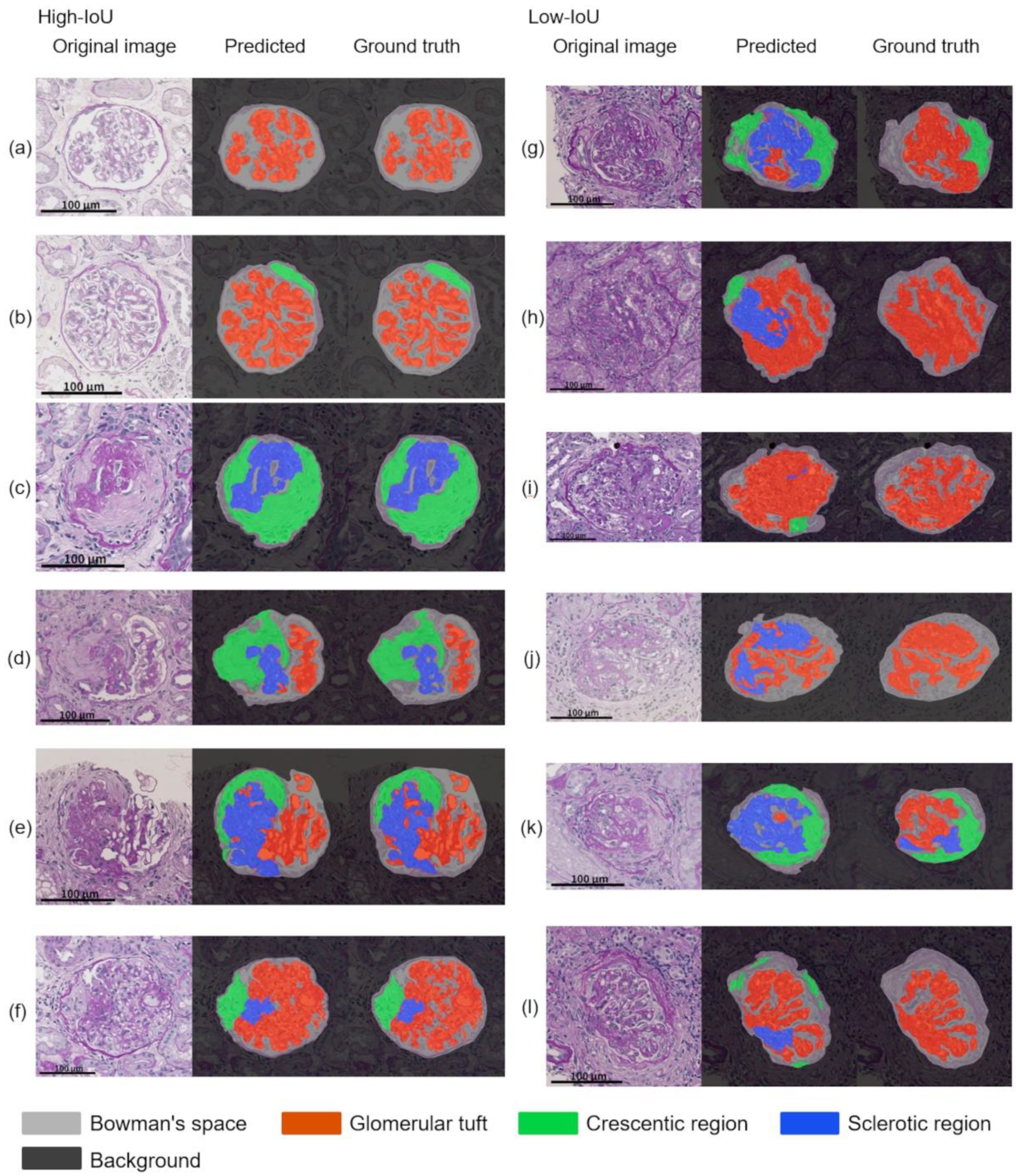
As shown in Table 4, the performance of the segmentation alone and the pipeline showed no significant differences in the mean IoU between T to T and K to K. This finding indicated that their internal performances were comparable. This finding supports that the annotation for glomerular detection and segmentation was conducted with a constant quality. Compared to the performance of the models that were trained with internal WSIs, the performance of the models that were trained with external WSIs tended to decrease in the segmentation alone and the pipeline. One of the reasons for this finding may be due to differences in the slide preparation to the digitization process between the facilities. The differences in the staining protocols, the manufacturing processes, and the digital scanner processing between the laboratories caused minute differences in the WSIs; however, the pathological samples were stained similarly. This difference is imperceptible to the human eye, but it is sufficient to affect deep learning-based applications [36,37,38]. We applied color normalization in the preprocessing step and Gaussian blurring, sharpening, and contrast changes during the data augmentation. However, extended methods are required in order to compensate for the minute differences in WSIs between the facilities, which increases the robustness against external WSI. The successful adaptation of WSI in deep neural network-based applications depends on each step of high-quality pathology slide preparation, such as embedding, cutting, staining, and scanning [39,40], as well as color variations. Using precise and homogeneous WSIs is desirable; however, such a model may not necessarily be robust against external WSIs that have more diversity. Improving the interfacility applicability of the developed model is an important issue for the success of deep learning applications in digital pathology. In addition, the performance of K to T is significantly lower for both the segmentation alone and the pipeline, while the performance degradations of T to K are not significant. This may be because a small number of glomerular images (1011) were used to develop the segmentation in model K, compared to the number of glomerular images that were used to develop model T (1713). We used the same number of WSIs from both of the facilities for the segmentation task. However, the number of images differed because of the different number of glomeruli that were contained in each WSI. The relatively small number of glomerular images in the training data for model K may have resulted in less diversity, leading to the significant performance degradation of K to T.

As shown in Table 5, the manually quantified (ground truth) sclerotic regions were associated with negatively impacting the eGFR slope in the multivariate analysis. Segmental sclerosis, which is defined by the Oxford Classification [5,6], or the chronic lesions including segmental sclerosis and global sclerosis, which are defined by the H-Grade [7,8] have a negative impact on the poor prognosis of IgAN; however, the current study showed that the quantified sclerotic regions also have a negative impact on the eGFR slope within two years after biopsy. In our analysis, the effect of the post-biopsy treatment on eGFR was not adjusted because of the retrospective design, which is a limitation of this analysis. In addition, other limitations of this analysis were that the 2-year period was relatively short and the number of IgAN cases (n = 46) was also limited; these may have affected the relatively low coefficients of determination (0.18 in the ground truth model).

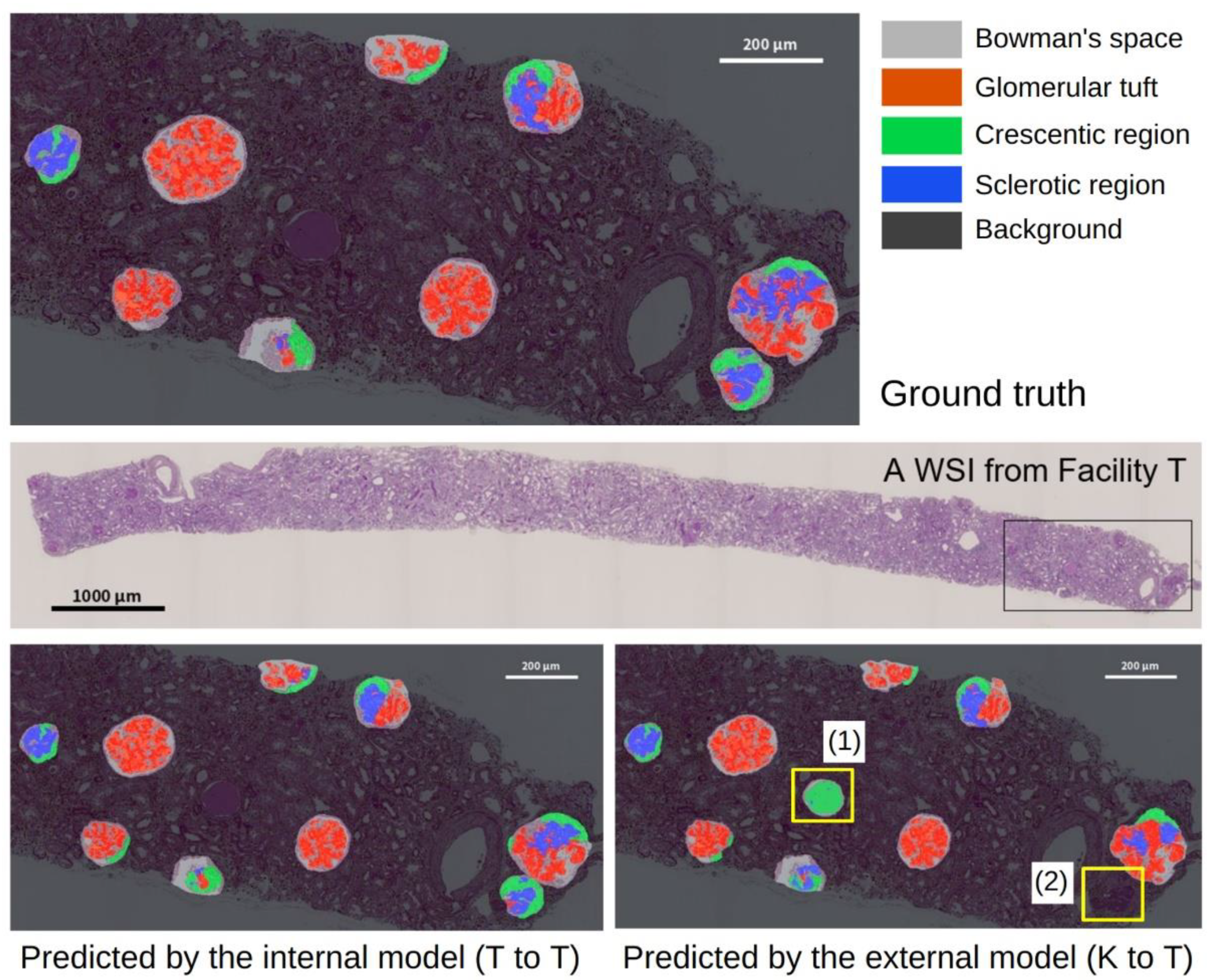
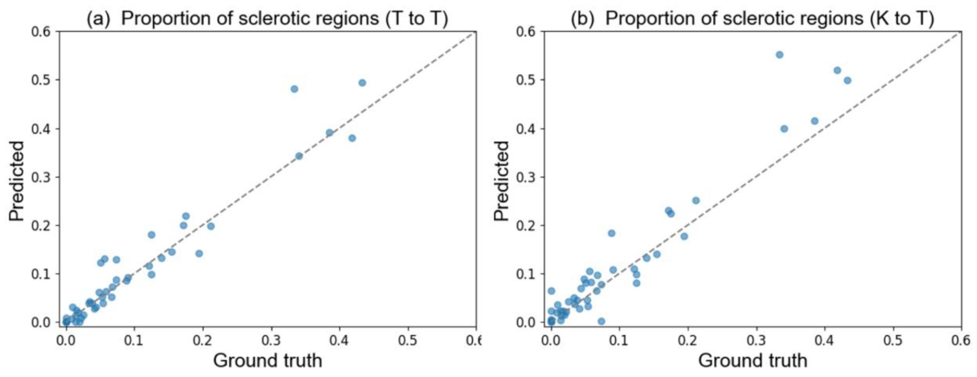
Table 5 also shows the same tendency in the standardized partial regression coefficients among the ground truth, the T to T (i.e., internal model), and the K to T (i.e., external model) models. The correlation between the ground truth regions and the predicted regions in each WSI aids in the understanding of their impact in the regression model. In Table A3 in Appendix E, the correlation coefficient for the sclerotic regions exceeded 0.96, even when using the external model. This finding indicated that the estimation of the total amount of sclerotic and glomerular tuft regions in each WSI was approximately correct. In light of the previous results, our developed pipeline shows a certain level of robustness for quantifying the glomerular tuft and sclerotic regions from WSI, even if the model is applied to the WSI of external facilities.

Another limitation of this study is that the concordance of the ground truth labels that have been used for developing glomerular detection and segmentation was not evaluated; however, the experts provided them. Surrounding the glomeruli with bounding boxes and drawing their histopathological components required distinguishing unclear boundaries with an understanding of pathology. Such labeling could vary among experts. Well-annotated examples are important in supervised learning; the main challenge in deep neural network-based applications for digital histopathology is obtaining high-quality labels. We carefully conducted the annotation with multiple experts, including a nephrologist and a pathologist, however the possibility of errors does exist. Nonetheless, annotation errors are not specific to this research; however, they should be kept in mind in studies on supervised learning.

5. Conclusions

We developed an automated computational pipeline for detecting glomeruli on PAS-stained WSIs, followed by segmenting the Bowman’s space, the glomerular tuft, the crescentic, and the sclerotic region inside of the glomeruli. The internal and external evaluation of the pipeline using WSIs from two facilities showed that the mean IoU of five regions, including the background, was 0.670 (T to T) and 0.693 (K to K) in the internal evaluation, and 0.609 (K to T) and 0.678 (T to K) in the external evaluation. The multivariate analysis for eGFR prognosis in cases of IgAN showed that the proportion of sclerotic regions that were quantified by the pipelines, even those that were quantified by the external model, had a significant negative impact on the eGFR slope, while five other clinical prognostic factors (i.e., age, sex, hypertension, eGFR at biopsy, and UPCR at biopsy) had no significant impact. These findings suggest the importance of quantifying the sclerotic region, as well as the usefulness and the robustness of the developed pipeline, for the purpose of predicting eGFR in cases of IgAN. The developed pipeline could aid in diagnosing renal pathology by visualizing and quantifying the histopathological feature of glomerulus. In addition, this high-throughput approach could potentially accelerate research in order to better understand the prognosis of IgAN.

References

1. Liyanage, T.; Ninomiya, T.; Jha, V.; Neal, B.; Patrice, H.M.; Okpechi, I.; Zhao, M.H.; Lv, J.; Garg, A.X.; Knight, J.; et al. Worldwide access to treatment for end-stage kidney disease: A systematic review. Lancet 2015, 385, 1975–1982. [Google Scholar] [CrossRef]
2. Magistroni, R.; D’Agati, V.D.; Appel, G.B.; Kiryluk, K. New developments in the genetics, pathogenesis, and therapy of IgA nephropathy. Kidney Int. 2015, 88, 974–989. [Google Scholar] [CrossRef] [Green Version]
3. Wyatt, R.J.; Julian, B.A. IgA nephropathy. N. Engl. J. Med. 2013, 368, 2402–2414. [Google Scholar] [CrossRef] [Green Version]
4. Yuzawa, Y.; Yamamoto, R.; Takahashi, K.; Katafuchi, R.; Tomita, M.; Fujigaki, Y.; Kitamura, H.; Goto, M.; Yasuda, T.; Sato, M.; et al. Evidence-based clinical practice guidelines for IgA nephropathy 2014. Clin. Exp. Nephrol. 2016, 20, 511–535. [Google Scholar] [CrossRef] [Green Version]
5. Working Group of the International IgA Nephropathy Network and the Renal Pathology Society; Roberts, I.S.; Cook, H.T.; Troyanov, S.; Alpers, C.E.; Amore, A.; Barratt, J.; Berthoux, F.; Bonsib, S.; Bruijn, J.A.; et al. The Oxford classification of IgA nephropathy: Pathology definitions, correlations, and reproducibility. Kidney Int. 2009, 76, 546–556. [Google Scholar] [CrossRef] [Green Version]
6. Trimarchi, H.; Barratt, J.; Cattran, D.C.; Cook, H.T.; Coppo, R.; Haas, M.; Liu, Z.H.; Roberts, I.S.; Yuzawa, Y.; Zhang, H.; et al. Oxford classification of IgA nephropathy 2016: An update from the IgA Nephropathy Classification Working Group. Kidney Int. 2017, 91, 1014–1021. [Google Scholar] [CrossRef] [Green Version]
7. Joh, K.; McNamara, K.M. Differences of histological classification between the Japanese histological grade classification and the Oxford classification. In Pathogenesis and Treatment in IgA Nephropathy; Tomino, Y., Ed.; Springer: Tokyo, Japan, 2016; pp. 69–87. [Google Scholar] [CrossRef]
8. Tomino, Y. Diagnosis and treatment of patients with IgA nephropathy in Japan. Kidney Res. Clin. Pract. 2016, 35, 197–203. [Google Scholar] [CrossRef]
9. Barisoni, L.; Troost, J.P.; Nast, C.; Bagnasco, S.; Avila-Casado, C.; Hodgin, J.; Palmer, M.; Rosenberg, A.; Gasim, A.; Liensziewski, C.; et al. Reproducibility of the Neptune descriptor-based scoring system on whole-slide images and histologic and ultrastructural digital images. Mod. Pathol. 2016, 29, 671–684. [Google Scholar] [CrossRef] [Green Version]
10. Yamaguchi, R.; Kawazoe, Y.; Shimamoto, K.; Shinohara, E.; Tsukamoto, T.; Shintani-Domoto, Y.; Nagasu, H.; Uozaki, H.; Ushiku, T.; Nangaku, M.; et al. Glomerular classification using convolutional neural networks based on defined annotation criteria and concordance evaluation among clinicians. Kidney Int. Rep. 2021, 6, 716–726. [Google Scholar] [CrossRef]
11. Simon, O.; Yacoub, R.; Jain, S.; Tomaszewski, J.E.; Sarder, P. Multi-radial LBP features as a tool for rapid glomerular detection and assessment in whole slide histopathology images. Sci. Rep. 2018, 8, 2032. [Google Scholar] [CrossRef] [Green Version]
12. Marée, R.; Dallongeville, S.; Olivo-Marin, J.-C.; Meas-Yedid, V. An approach for detection of glomeruli in multisite digital pathology. In Proceedings of the 2016 IEEE 13th International Symposium on Biomedical Imaging (ISBI), Prague, Czech Republic, 13–16 April 2016; pp. 1033–1036. [Google Scholar] [CrossRef] [Green Version]
13. Kawazoe, Y.; Shimamoto, K.; Yamaguchi, R.; Shintani-Domoto, Y.; Uozaki, H.; Fukayama, M.; Ohe, K. Faster R-CNN-based glomerular detection in multistained human whole slide images. J. Imaging. 2018, 4, 91. [Google Scholar] [CrossRef] [Green Version]
14. Temerinac-Ott, M.; Forestier, G.; Schmitz, J.; Hermsen, M.; Brasen, J.H.; Feuerhake, F.; Wemmert, C. Detection of glomeruli in renal pathology by mutual comparison of multiple staining modalities. In Proceedings of the 10th International Symposium on ISPA, Ljubljana, Slovenia, 18–20 September 2017; pp. 19–24. [Google Scholar] [CrossRef]
15. Uchino, E.; Suzuki, K.; Sato, N.; Kojima, R.; Tamada, Y.; Hiragi, S.; Yokoi, H.; Yugami, N.; Minamiguchi, S.; Haga, H.; et al. Classification of glomerular pathological findings using deep learning and nephrologist-AI collective intelligence approach. Int. J. Med. Inform. 2020, 141, 104231. [Google Scholar] [CrossRef]
16. Kato, T.; Relator, R.; Ngouv, H.; Hirohashi, Y.; Takaki, O.; Kakimoto, T.; Okada, K. Segmental HOG: New descriptor for glomerulus detection in kidney microscopy image. BMC Bioinform. 2015, 16, 316. [Google Scholar] [CrossRef] [PubMed]
17. Gallego, J.; Pedraza, A.; Lopez, S.; Steiner, G.; Gonzalez, L.; Laurinavicius, A.; Bueno, G. Glomerulus classification and detection based on convolutional neural networks. J. Imaging. 2018, 4, 20. [Google Scholar] [CrossRef] [Green Version]
18. Ginley, B.; Lutnick, B.; Jen, K.Y.; Fogo, A.B.; Jain, S.; Rosenberg, A.; Walavalkar, V.; Wilding, G.; Tomaszewski, J.E.; Yacoub, R.; et al. Computational segmentation and classification of diabetic glomerulosclerosis. J. Am. Soc. Nephrol. 2019, 30, 1953–1967. [Google Scholar] [CrossRef]
19. Hermsen, M.; de Bel, T.; den Boer, M.; Steenbergen, E.J.; Kers, J.; Florquin, S.; Roelofs, J.J.T.H.; Stegall, M.D.; Alexander, M.P.; Smith, B.H.; et al. Deep learning-based histopathologic assessment of kidney tissue. J. Am. Soc. Nephrol. 2019, 30, 1968–1979. [Google Scholar] [CrossRef]
20. Bueno, G.; Fernandez-Carrobles, M.M.; Gonzalez-Lopez, L.; Deniz, O. Glomerulosclerosis identification in whole slide images using semantic segmentation. Comput. Methods Programs Biomed. 2020, 184, 105273. [Google Scholar] [CrossRef]
21. Altini, N.; Cascarano, G.D.; Brunetti, A.; Marino, F.; Rocchetti, M.T.; Matino, S.; Venere, U.; Rossini, M.; Pesce, F.; Gesualdo, L.; et al. Semantic segmentation framework for glomeruli detection and classification in kidney histological sections. Electronics 2020, 9, 503. [Google Scholar] [CrossRef] [Green Version]
22. Zeng, C.; Nan, Y.; Xu, F.; Lei, Q.; Li, F.; Chen, T.; Liang, S.; Hou, X.; Lv, B.; Liang, D.; et al. Identification of glomerular lesions and intrinsic glomerular cell types in kidney diseases via deep learning. J. Pathol. 2020, 252, 53–64. [Google Scholar] [CrossRef] [PubMed]
23. Bouteldja, N.; Klinkhammer, B.M.; Bülow, R.D.; Droste, P.; Otten, S.W.; Freifrau von Stillfried, S.; Moellmann, J.; Sheehan, S.M.; Korstanje, R.; Menzel, S.; et al. Deep learning–based segmentation and quantification in experimental kidney histopathology. J. Am. Soc. Nephrol. 2021, 32, 52–68. [Google Scholar] [CrossRef]
24. Jiang, L.; Chen, W.; Dong, B.; Mei, K.; Zhu, C.; Liu, J.; Cai, M.; Yan, Y.; Wang, G.; Zuo, L.; et al. A deep learning-based approach for glomeruli instance segmentation from multistained renal biopsy pathologic images. Am. J. Pathol. 2021, 191, 1431–1441. [Google Scholar] [CrossRef]
25. Ren, S.; He, K.; Girshick, R.; Sun, J. Faster R-CNN: Towards real-time object detection with region proposal networks. IEEE Trans. Pattern Anal. Mach. Intell. Proc. 2017, 39, 1137–1149. [Google Scholar] [CrossRef] [Green Version]
26. Xie, E.; Wang, W.; Yu, Z.; Anandkumar, A.; Alvarez, J.M.; Luo, P. SegFormer: Simple and efficient design for semantic segmentation with transformers. Adv. Neural Inf. Process. Syst. 2021, 34, 12077–12090. [Google Scholar] [CrossRef]
27. Vaswani, A.; Shazeer, N.; Parmar, N.; Uszkoreit, J.; Jones, L.; Gomez, A.; Kaiser, L.; Polosukhin, I. Attention is all you need. In Proceedings of the NIPS, Long Beach, CA, USA, 4–7 December 2017; pp. 5998–6008. [Google Scholar] [CrossRef]
28. Van Pottelbergh, G.; Den Elzen, W.P.; Degryse, J.; Gussekloo, J. Prediction of mortality and functional decline by changes in eGFR in the very elderly: The Leiden 85-plus study. BMC Geriatr. 2013, 13, 61. [Google Scholar] [CrossRef] [Green Version]
29. Turin, T.C.; Coresh, J.; Tonelli, M.; Stevens, P.E.; de Jong, P.E.; Farmer, C.K.; Matsushita, K.; Hemmelgarn, B.R. Change in the estimated glomerular filtration rate over time and risk of all-cause mortality. Kidney Int. 2013, 83, 684–691. [Google Scholar] [CrossRef] [Green Version]
30. Vaes, B.; Beke, E.; Truyers, C.; Elli, S.; Buntinx, F.; Verbakel, J.Y.; Goderis, G.; Van Pottelbergh, G. The correlation between blood pressure and kidney function decline in older people: A registry-based cohort study. BMJ Open. 2015, 5, e007571. [Google Scholar] [CrossRef]
31. Naimark, D.M.J.; Grams, M.E.; Matsushita, K.; Black, C.; Drion, I.; Fox, C.S.; Inker, L.A.; Ishani, A.; Jee, S.H.; Kitamura, A.; et al. Past decline versus current eGFR and subsequent mortality risk. J. Am. Soc. Nephrol. 2016, 27, 2456–2466. [Google Scholar] [CrossRef] [Green Version]
32. Oshima, M.; Jun, M.; Ohkuma, T.; Toyama, T.; Wada, T.; Cooper, M.E.; Hadjadj, S.; Hamet, P.; Harrap, S.; Mancia, G.; et al. The relationship between eGFR slope and subsequent risk of vascular outcomes and all-cause mortality in type 2 diabetes: The ADVANCE-ON study. Diabetologia 2019, 62, 1988–1997. [Google Scholar] [CrossRef] [Green Version]
33. Inker, L.A.; Heerspink, H.J.L.; Tighiouart, H.; Levey, A.S.; Coresh, J.; Gansevoort, R.T.; Simon, A.L.; Ying, J.; Beck, G.J.; Wanner, C.; et al. GFR Slope as a surrogate end point for kidney disease progression in clinical trials: A meta-analysis of treatment effects of randomized controlled trials. J. Am. Soc. Nephrol. 2019, 30, 1735–1745. [Google Scholar] [CrossRef]
34. Badrinarayanan, V.; Kendall, A.; Cipolla, R. SegNet: A deep convolutional encoder-decoder architecture for image segmentation. IEEE Trans. Pattern Anal. Mach. Intell. 2017, 39, 2481–2495. [Google Scholar] [CrossRef]
35. Ronneberger, O.; Fischer, P.; Brox, T. U-Net: Convolutional Networks for Biomedical Image Segmentation; Miccai, N.N., Ed.; Springer: Cham, Switzerland, 2015; pp. 234–241. [Google Scholar] [CrossRef] [Green Version]
36. Dimitriou, N.; Arandjelović, O.; Caie, P.D. Deep learning for whole slide image analysis: An overview. Front. Med. 2019, 6, 264. [Google Scholar] [CrossRef] [Green Version]
37. Khened, M.; Kori, A.; Rajkumar, H.; Krishnamurthi, G.; Srinivasan, B. A generalized deep learning framework for whole-slide image segmentation and analysis. Sci. Rep. 2021, 11, 11579. [Google Scholar] [CrossRef]
38. Bansal, R.; Raj, G.; Choudhury, T. Blur Image Detection Using Laplacian Operator and Open-CV. In Proceedings of the 2016 International Conference System Modeling & Advancement in Research Trends (SMART), Moradabad, India, 25–27 November 2016. [Google Scholar] [CrossRef]
39. Cui, M.; Zhang, D.Y. Artificial intelligence and computational pathology. Lab. Investig. 2021, 101, 412–422. [Google Scholar] [CrossRef]
40. Serag, A.; Ion-Margineanu, A.; Qureshi, H.; McMillan, R.; Saint Martin, M.J.; Diamond, J.; O’Reilly, P.; Hamilton, P. Translational AI and deep learning in diagnostic pathology. Front. Med. 2019, 6, 185. [Google Scholar] [CrossRef]
41. SegFormer. Available online: https://huggingface.co/docs/transformers/model_doc/segformer#segformer (accessed on 8 November 2022).
Figure 1. Example of a whole slide image (WSI) (top row). The bounding boxes of a glomerulus are shown as a rectangle with a yellow border in the second row. The glomerular images cropped by the bounding boxes are shown in the third row. The annotated images for the segmentation corresponding to the cropped glomeruli are shown in the bottom row. The examples in the (bottom row) (1)–(4) include cases with different percentages of sclerotic regions. (1) is an example of global sclerosis, in which there is no glomerular tuft (red). (2) and (3) are examples without sclerosis, in which there is no sclerotic region (blue). (4) is an example of segmental sclerosis, in which the glomerular tuft (red) and sclerotic region (blue) are almost equal in area.
Diagnostics 12 02955 g001
Figure 2. Overview of the computational pipeline. The parallelograms indicate the input or output data. The rectangles indicate the process. Faster R-CNN is described by Ren et al. [25], and SegFormer is described by Xie et al. [26].
Diagnostics 12 02955 g002
Figure 3. Example of the results of a whole slide image (WSI) from facility T. Top: manually annotated glomeruli and their components (i.e., ground truth). Middle: The WSI of the renal sample. The box is the area depicted in the top and bottom images. Bottom left: The predicted result obtained by model T (i.e., internal model). Bottom right: The predicted result obtained by model K (i.e., external model). In the example of the predicted result in the bottom right (K to T), (1) a dilated tubule filled with Tamm–Horsfall protein is incorrectly detected as glomerulus, and (2) a glomerulus is undetected, both of which are due to errors that occurred in the detection process in the first step of the computational pipeline.
Diagnostics 12 02955 g003
Figure 4. Example of the glomerular component segmentation obtained by the pipeline of K to T (predicted by the external model). The left column shows examples with higher mean intersection over union (IoU) of (a) 0.894, (b) 0.879, (c) 0.846, (d) 0.818, (e) 0.792, and (f) 0.780. The right column shows examples with lower mean IoU of (g) 0.377, (h) 0.384, (i) 0.412, (j) 0.417, (k) 0.438, and (l) 0.453. In the right column (af), the Bowman’s space, glomerular tuft, crescentic, and sclerotic region are correctly segmented. The pairs of the proportions of the sclerotic region of ground truth that are predicted in left column are (ac) 0.0 to 0.0, (d) 0.485 to 0.446, (e) 0.451 to 0.518, and (f) 0.085 to 0.101, which are generally corresponding. (g) Most of the glomerular tuft region is incorrectly segmented as the sclerotic region, and the left side of the Bowman’s spaces are incorrectly segmented to the crescentic regions. (h) The left side of the glomerular tuft region is incorrectly segmented to the sclerotic region, and the upper left Bowman’s space is incorrectly segmented as the crescentic region. (i) The Bowman’s spaces in the glomerular tuft gaps are incorrectly segmented as the glomerular tuft areas, and the bottom of the glomerular tuft is incorrectly segmented as the crescentic regions. (j) The upper and lower left glomerular tuft areas are incorrectly segmented as the sclerotic regions. (k) Most of the glomerular tuft region from the upper left to the center is incorrectly segmented to the sclerotic region. (l) The lower left glomerular tuft region near the vascular pole is incorrectly segmented to the sclerotic region, and several small regions around the Bowman’s space are incorrectly segmented to the crescentic regions. The pairs of the proportions of the sclerotic region of ground truth that are predicted in right column are (g) 0.0 to 0.832, (h) 0.0 to 0.282, (i) 0.0 to 0.009, (j) 0.0 to 0.430, (k) 0.247 to 0.967, and (l) 0.0 to 0.158. All scale bars indicate 100 mm.
Diagnostics 12 02955 g004