Homogeneous Continuous-Time, Finite-State Hidden Semi-Markov Modeling for Enhancing Empirical Classification System Diagnostics of Industrial Components

Abstract

This work presents a method to improve the diagnostic performance of empirical classification system (ECS), which is used to estimate the degradation state of components based on measured signals. The ECS is embedded in a homogenous continuous-time, finite-state semi-Markov model (HCTFSSMM), which adjusts diagnoses based on the past history of components. The combination gives rise to a homogeneous continuous-time finite-state hidden semi-Markov model (HCTFSHSMM). In an application involving the degradation of bearings in automotive machines, the proposed method is shown to be superior in classification performance compared to the single-stage ECS.

1. Introduction

Multistate degradation modeling has been receiving considerable attention for supporting dynamic maintenance paradigms based on condition monitoring (CM), such as condition-based maintenance and predictive maintenance (examples in References [1,2,3,4]). In fact, multistate models describe the degradation evolution more realistically than binary models, as the evolution of many degradation processes proceed in successive phases characterized by different physical degradation mechanisms. For example, the crack growth degradation mechanism of a mechanical component subject to cyclic loads is typically modeled as a four-state degradation process in which different degradation mechanisms take place [5,6].

A further reason for the growing interest in multistate degradation models is their proximity to the maintenance data acquired in the field from operating systems. For example, operators typically assign a qualitative tag to equipment health during periodic inspections. Multistate modeling has also been adopted to describe the evolution of degradation in membranes of pumps operated in nuclear power plants [7], in turbine nozzles for the oil and gas industry [8], in components of the electrical industry [9,10], liners of marine diesel engine cylinders [2,11], and piping of nuclear power plants [12].

Finally, a strong advantage of multistate degradation models is that they exploit sound, well-established mathematical techniques for their quantification, such as the Markov and semi-Markov models. In particular, when CM data are available, the hidden semi-Markov process (HSMP) theory offers a full-fledged framework for building a multistate degradation model while handling the two uncertainties involved: (a) the observation process, which relates the CM data to the actual, but hidden, degradation state of the component; and (b) the multistate degradation process of the component.

In the literature, many authors have tackled the problem of assessing the degradation state of aging multistate components by resorting to hidden Markov models (HMMs) or hidden semi-Markov models (HSMMs). References [3,13,14,15] provide some examples. However, all these works disregarded the engineering issue of building a classifier from CM data, which is the aim of this work. Rather, they sought to estimate the performance of this classifier as inferred from available sequences of observation of degradation trajectories. In this way, they assumed that there is a one-to-one correspondence between component degradation and a single feature extracted from the data, which is a priori known. However, this situation may be not be typical in several practical cases where a direct measure of component degradation is not available, and a feature selection from monitored signals [16] is required to identify features that are relevant for building an effective classifier of the equipment degradation state. For example, when dealing with bearings mounted on the powertrain of machinery [17,18], the available condition monitored data are vibrational signals from which a large number of features can be extracted, and a combination of them is required to infer the observed degradation state [19].

The diagnostic issue of building a classifier based on features to be embedded in a HSMM is considered in References [20,21]. To do this, the authors used a mixture of log-concave, elliptical, or symmetric continuous probability density functions (pdfs) (e.g., mixture of Gaussians) to describe the uncertainty of having a given vector of features and the actual degradation state of the component. The limitations of this approach stem from the large number of parameters that need to be estimated. For example, if the semi-Markov degradation process has $N=4$ states and the optimal combination of features is made of $n=10$ elements, then $n=10$ mean values and $n\left(n+1\right)/2=55$ values of the covariance matrix needs to be estimated for each of the $N=4$ states, i.e., a total of $55\times 4=220$ parameters. This is a computationally burdensome approach that requires a very large dataset to infer the parameter values. Moreover, as mentioned above, some restrictions on the form of the model pdfs hold.

The main contribution of this paper is to develop a novel hybrid scheme for diagnosing the degradation state of monitored components, which integrates a robust, largely applicable empirical classification system (ECS) with the homogeneous continuous-time finite-state hidden semi-Markov model (HCTFSHSMM) framework. This combination gives rise to a new diagnostic tool that improves the current estimation of ECS using the observed path of component degradation. The proposed approach is detailed in the next subsection.

Methodology Snapshot

We assume that the information available for the development of the hybrid diagnostic approach is constituted by a dataset containing K-tested similar components of the pairs signal measurements-corresponding degradation state, collected during the entire degradation trajectory of every tested component, from the beginning of its life to the failure. These pairs are used to build an ECS (see Section 2.1). However, the limitation of ECSs for fault diagnostics is that their classification outputs are static, i.e., the class assignment process is independent of the actual stochastic dynamics of the degradation process whereby the information content about the component degradation history is lost.

To overcome this limitation, we propose to combine ECS with a homogeneous continuous-time finite-state semi-Markov model (HCTFSSMM), thus obtaining a HCTFSHSMM. The underlying degradation process is modeled as HCTFSSMM, which is called “hidden” because the information about the component degradation state is not directly known. The ECS is framed as the observation process of the HCTFSHSMM. The classification performance of ECS on a set of pairs signal measurements-corresponding degradation state not previously employed to build the classifier forms the observation matrix, containing the probabilities that a component in a given state $i$ is assigned by the ECS to the degradation state $j$, for any possible $i$ and $j\in E$, where $E$ is the finite set of degradation states.

Then, maximum likelihood estimation (MLE) is applied to infer the parameters of the underlying HCTFSHSMM from the sequences of classification labels provided by the ECS on a given set of training trajectories. This way, the proposed procedure uses the output of the built ECS as input data for the estimation of the remaining parameters of the HCTFSHSMM.

The obtained HCTFSHSMM-based diagnostic system estimates the degradation state of a test component as that with the largest probability of being occupied. Therefore, the HCTFSHSMM works like a corrector of the classifications provided by the ECS because it also takes into account previous observations and parameters of the stochastic degradation process. Therefore, the degradation state provided by the developed semi-Markov model is more accurate than that provided by the ECS.

This solution, which is the main contribution of the present work, has an additional computational advantage. The model frames the classification performance of ECS as the entries of the observation matrix avoid developing an algorithm for estimating the value of its entries, as proposed by Moghaddass and Zuo [3]. This reduces the number of parameters that need to be estimated within the HCTFSHSSM framework and hence the data and the computational effort required to set the HCTFSHSSM.

The proposed methodology is shown using the example of degradation of bearings mounted on electrical machines. This is based on our previous work [22].

The remainder of the paper is organized as follows: Section 2 introduces the hybrid diagnostic system for degradation state assessment; Section 3 illustrates techniques to estimate hidden model parameters in the specific context in which the observation matrix is known. Section 4 shows the method to assess on-line the current degradation state of the equipment. In Section 5, a case study and the application of the proposed method are presented. The limitations of the proposed methodology and its possible developments are discussed in Section 6. Finally, Section 7 outlines the conclusions of the work.

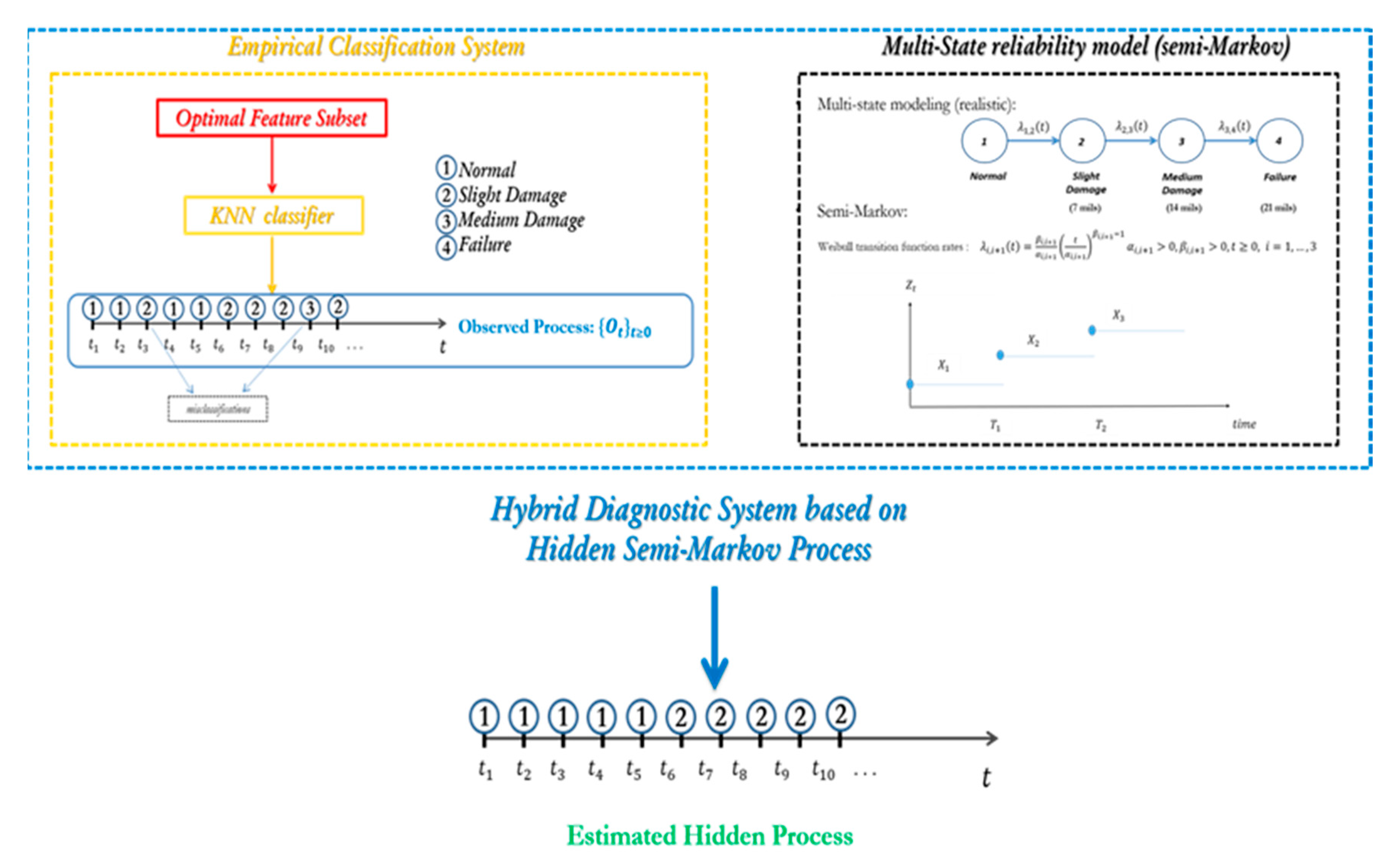
2. The Hybrid Diagnostic Approach

In this section, we describe the hybrid diagnostic approach. In Section 2.1, a general framework to develop an ECS within the feature-driven approach is presented. Section 2.2 discusses multistate semi-Markov processes for degradation modeling. Finally, in Section 2.3 and Section 2.4, the HCTFSHSMM—which combines the ECS with multistate semi-Markov processes for degradation state assessment—is presented.

2.1. Development of the ECS within the Feature-Driven Approach

We assume to have available a training set containing measurements performed on similar components in different degradation states. These data are used to develop an ECS for identification of the equipment degradation state, i.e., to establish the relationship between measured signals and degradation state. The classification algorithm is developed within a feature-driven framework [23] through the following general procedure [22]:

(1)

The extraction of features from the raw measurements [24]. To do this, we rely on the strategy discussed by Cannarile et al. [25].

(2)

The selection of an optimal subset of relevant features to be used for the classification [26] through the scheme proposed in our earlier work [22], i.e., the feature selector behaves as a wrapper around the specific learning algorithm used to construct the classifier [16]. The objective functions used for evaluating and comparing the feature subsets during the search are the recognition rate achieved by the ECS (to be maximized) and the number of features forming the subsets (to be minimized). This way, the feature selection problem is formulated as a multiobjective optimization problem [27]. As the large number of extracted features makes it infeasible for an exhaustive search, we use a binary differential evolution (BDE) [28], which has been shown to explore the decision space more efficiently compared to other multiobjective evolutionary algorithms [29] such as non-dominated sorting genetic algorithm II (NSGA-II) [30], strength Pareto evolutionary algorithm (SPEA2) [31], and indicator-based evolutionary algorithm (IBEA) [32].

(3)

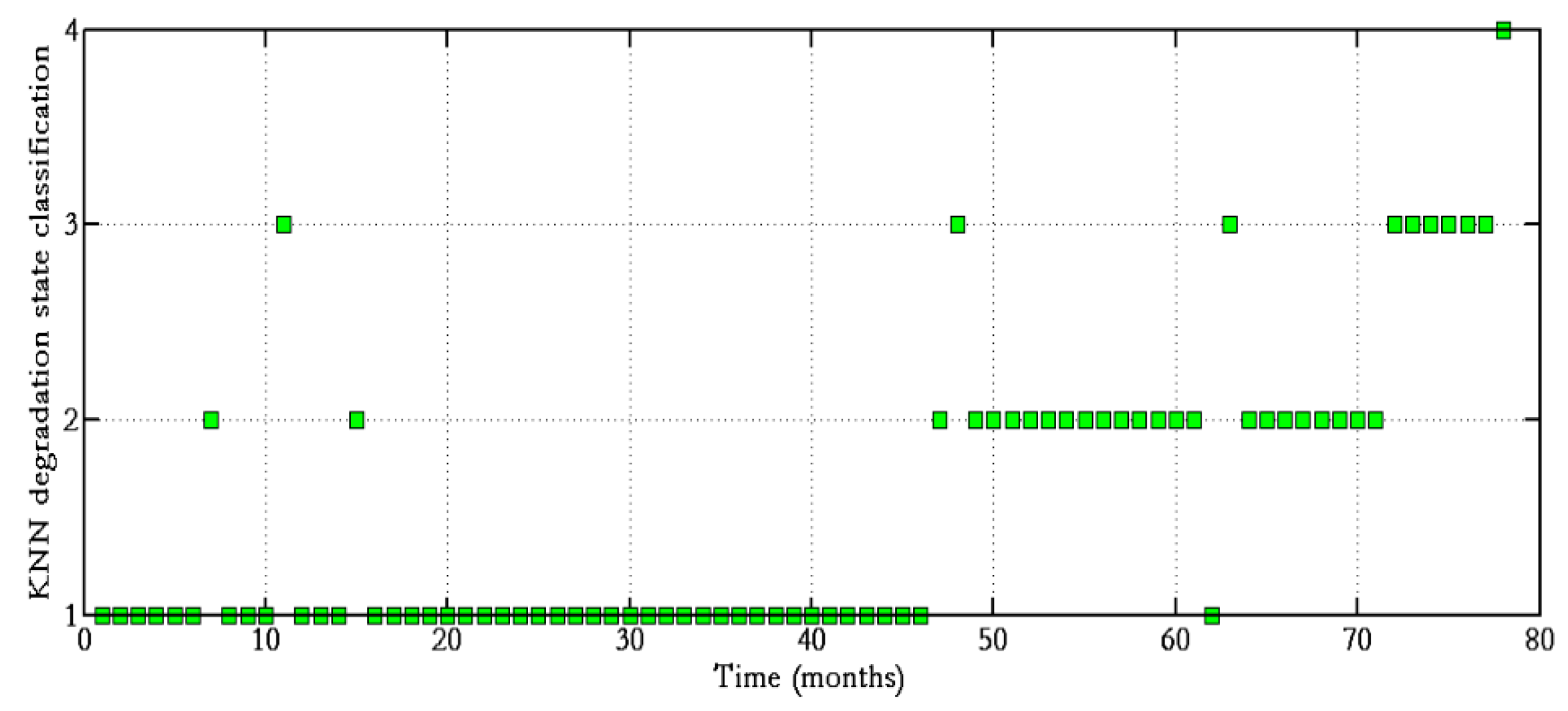
The development of the empirical classifier. A k-nearest neighbors (KNN) is used as the classification algorithm [33,34]. This choice is justified by the following advantages: (1) KNN requires setting few parameters and (2) it does not require the classes to be linearly separable in the input space.

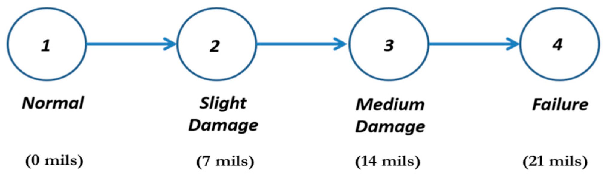
2.2. Degradation Modeling Based on Homogeneous Continuous-Time Finite State Semi-Markov Processes

We assume that the degradation states are regeneration states, i.e., when the ith state is reached, the previous history of the process can be neglected as it has no influence on the future degradation evolution. This assumption is made by several models of degradation phenomena, such as the Paris–Erdogan model [35]. This class of processes is called homogenous processes and is usually further divided into two main categories:

• Markov models, in which the sojourn times in the states are exponentially distributed and the transition rates are constant.
• Semi-Markov models, where the transition rates depend on the time spent in the current state. In semi-Markov models, the transition occurrences depend on the sojourn times, which can follow arbitrary distributions. In this work, we assume that they are Weibull distributions, as these are the probability distributions most commonly used to describe the degradation processes of industrial components [3,36].

As anticipated above, we assume that the real degradation state of the equipment is not directly observable on-line and that the available information comes from the ECS described in Section 2.1, which classifies the equipment degradation state. Furthermore, the classification performance of the ECS is assumed to be known. Hence, the resulting degradation model is framed as a hidden semi-Markov process [4,37,38,39,40] with known misclassification probabilities.

Finally, the process is assumed to be a left-to-right process, that is, at time $t=0$ the equipment is always in an ‘as good as new’ (AGAN) condition (i.e., not degraded). Once it starts degrading, it is modeled by jumps from less degraded states to more degraded states, with the last state being equipment failure. More details on semi-Markov model are provided in Appendix A.

2.3. Hidden Semi-Markov Model for Degradation Assessment

The idea behind the use of a hidden model lies in the fact that we are interested in the evolution of the process $\{Z_t,t\ge 0\}$, which is hidden, i.e., it cannot be directly observed. Formally,

$$Z_t:\Omega \to E,E=\left\{1,\dots ,N\right\};t\in {ℝ}_{+}$$

(1)

where $\Omega$ is the sample space and $E$ is the state space.

Indeed, we can observe the evolution of another process—the observed process, $\left\{O_t,t\ge 0\right\}$

$$O_t:\Omega \to W,W=\left\{o_1,\dots ,o_M\right\};t\in {ℝ}_{+}$$

(2)

which is related to $Z_t$ in that the state in which the process is observed depends on the state of the hidden process [40].

This work builds on the work of Moghaddass and Zuo [3] to propose a hybrid method for the identification of the degradation state (Figure 1), namely, HCTFSHSMM embeds the ECS diagnostic system, which is framed as the observation process that links the actual degradation state with its corresponding on-line estimation based on sensor signals. This way, the proposed procedure uses the output of an ECS as input data for the HCTFSHSMM.

$$b_i\left(o\right)=\mathbb{P}(O_t=o|Z_t=i)i\in E;o\in W$$

(3)

Notice that without loss of generality, we assume that the number of observed states is equal to that of the actual state (i.e., $E\equiv W)$.

Finally, notice that a hybrid diagnostic system has been proposed also by Narasimhan et al. [23], which combined model-based and feature-driven diagnosis approaches. However, in contrast to that system, our hybrid diagnostic system is developed based on data only and therefore does not require building a first principle model (FPM) of the component functioning in nominal conditions.

2.4. HCTFSHSMM for Degradation Modeling

The objective of this subsection is to use the HCTFSHSMM modeling approach to improve the classification performance of an ECS. To do this, we address the following issues:

• Estimation of the model parameters, i.e., the parameters of the transition rate functions. This issue arises during the development of the hybrid diagnostic model.
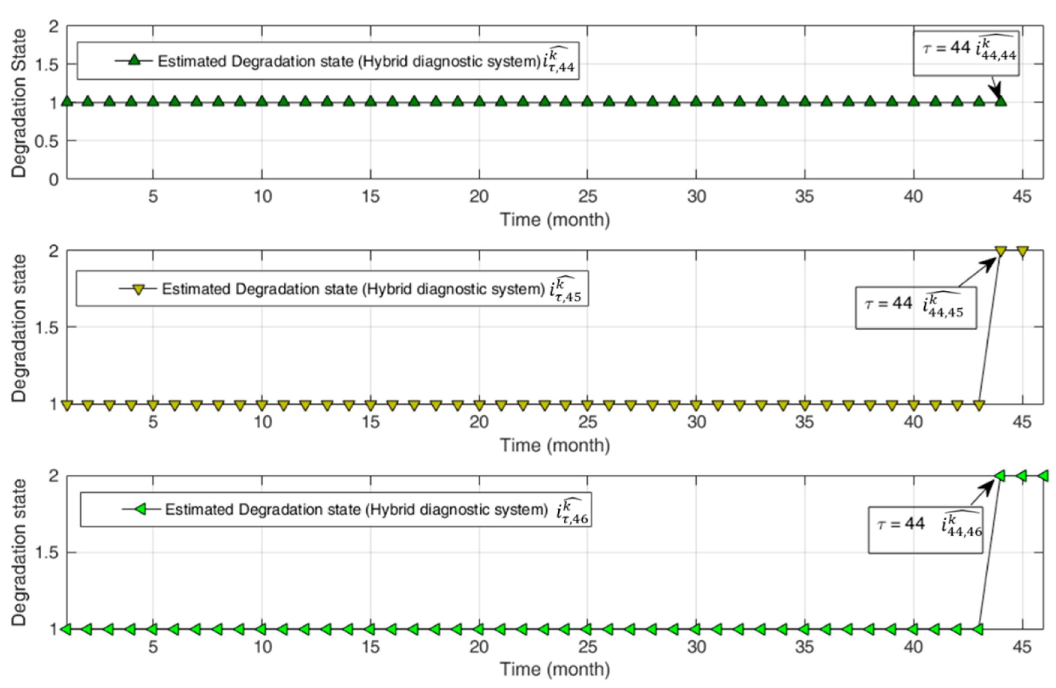
• Estimation of the most likely degradation state at the current time $t$, given the sequence of observations. This issue arises when the developed diagnostic model is used for assessing the degradation state of a test component of interest.

The following assumptions hold:

• At time $t=0,$ the component is not degraded, i.e., it is in state 1.
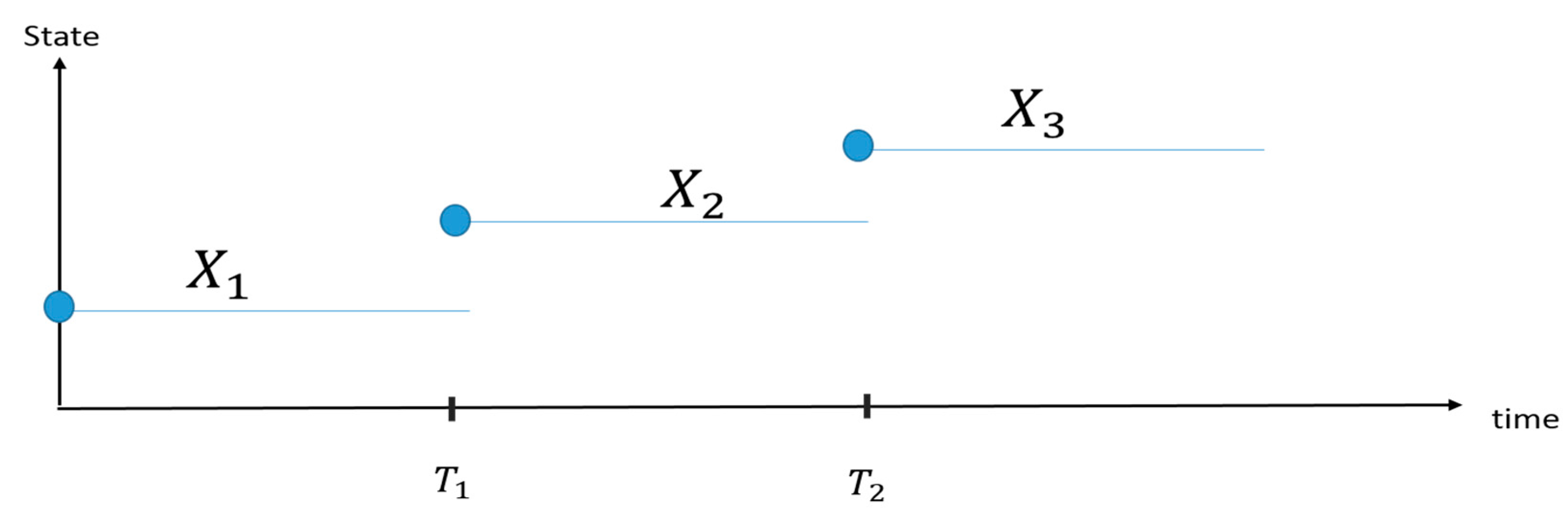
• The data available to estimate the model parameters are sequences of observations $\left\{O_1^k,O_2^k,\dots ,O_{l_k}^k\right\}$, which represent the outcomes of the KNN classifier taken at times $\{t_1^k,t_2^k,\dots ,t_{l_k}^k\}$, where the superscript $k$ refers to the sequence of observations, $k=1,\dots ,K$.
• The number $N$ of degradation states is known, $Z_t\in \left\{1,\dots ,N\right\},t\in {ℝ}_{+}$.
• The acquisition time period $\Delta =t_{\tau +1}^k-t_{\tau }^k$ is constant, $k=1,\dots ,K$ and $\tau =1,\dots ,l_k$. For simplicity, but with no loss of generality, we suppose $\Delta =1$; then, the equations presented in the next sections can be easily extended to the more general case.
• Just one transition can occur in the time interval $\Delta$.
• The last observation of each time series coincides with the failure of the component, which is directly observed.
• No maintenance and repair operations are considered; transitions only go left-to-right across the states.
• The ECS presented in Section 2.1 has been developed to assess the degradation state of the equipment. The misclassification probabilities $b_{i,j},i,j\in \left\{1,\dots ,N\right\}$ of the KNN classification algorithm are estimated by testing the performance of the diagnostic system on degradation patterns for which the actual degradation state is known. The values of the $b_{i,j}$ probabilities are then considered as the entries of the observation matrix $B$.

3. Maximum Likelihood Estimation of the Transition Function Rates

Suppose we have $K$ independent sample paths of observations ${\mathit{O}}^k=\{O_1^k,\dots ,O_{l_k}^k\}$. Then, the likelihood of gathering them is given by:

$$L\left({\mathit{O}}^1,\dots ,{\mathit{O}}^K|\mathit{\theta }\right)={{\displaystyle \prod }}_{k=1}^K\mathbb{P}({\mathit{O}}^k|\mathit{\theta })$$

(4)

where $\mathit{\theta }\in \mathbf{\Theta }$ are the unknown model parameters, and $\mathbb{P}\left({\mathit{O}}^k|\mathit{\theta }\right)$ is the probability of observing the sequence ${\mathit{O}}^k,$ given the value of $\mathit{\theta }$. The MLE is given by:

$$\widehat{{\mathit{\theta }}_{MLE}}=\underset{\mathit{\theta }\in \mathbf{\Theta }}{\mathrm{argmax}}L\left({\mathit{O}}^1,\dots ,{\mathit{O}}^K|\mathit{\theta }\right)$$

(5)

Maximizing likelihood (Equation (4)) is equivalent to maximizing the following log-likelihood function:

$$\log L\left({\mathit{O}}^1,\dots ,{\mathit{O}}^K|\mathit{\theta }\right)={\sum }_{k=1}^K\log \mathbb{P}({\mathit{O}}^k|\mathit{\theta })$$

(6)

Since Equation (6) cannot be written in closed form, the procedure proposed by Rabiner [14] and adapted by Moghaddass and Zuo [3] is typically adopted to treat the nonhomogeneous semi-Markov processes. The probabilities $\mathbb{P}$(${\mathit{O}}^k\left|\mathit{\theta }\right)$ are written in terms of the forward probabilities:

$${\alpha }_t^k\left(i\right)=\mathbb{P}({\mathit{O}}_{1:t}^k,Z_t^k=i|\mathit{\theta })t=1,\dots ,l;i=1,\dots ,N;k=1,\dots ,K$$

(7)

where ${\mathit{O}}_{1:t}^k=\left\{O_1^k,\dots ,O_t^k\right\}.$ From Equation (7) it follows that

$$\mathbb{P}\left(O_{1:t}^k\right|\mathit{\theta })={\sum }_{i=1}^N{\alpha }_t^k\left(i\right)t=1,\dots ,l_k;k=1:K$$

(8)

and

$$\log L\left({\mathit{O}}^1,\dots ,{\mathit{O}}^K|\mathit{\theta }\right)={\sum }_{k=1}^K\log ({\sum }_{i=1}^N{\alpha }_{l_k}^k\left(i\right))$$

(9)

More details on forward probabilities computation are provided in References [3,40,41]. To maximize Equation (6), we use the differential evolution (DE) algorithm [42]. According to Moghaddass and Zuo [3], the transition times, which are continuous variables, are discretized into time channels corresponding to the observation intervals [3]. We assume that these time intervals are short enough so that assumption V in Section 2.4 is not violated. The most significant consequence of the discretization concerns the estimation of the parameters. To see this, assume that we can perfectly observe the degradation process $Z_{\tau }^k$, $\tau =1,\dots ,l_k,k=1,\dots ,K$. If the transition from state $i$ to state $i+1$ occurs just after the $({\tau }_{i\to i+1}^k$)-th inspection time, the event will be recorded only at time instant $t_{({\tau }_{i\to i+1}^k)+1}^k={\tau }_{({\tau }_{i\to i+1}^k)}^k+\Delta$. Consequently, the observed sojourn time in state $i$ of the $k^{th}$ component, ${\mu }_i^k,$ is subject to interval censoring [43]: ${\mu }_i^k\in \left[{\tau }_{({\tau }_{i\to i+1}^k)}^k-\left({\tau }_{({\tau }_{i-1\to i}^k)}^k+\Delta \right),{\tau }_{({\tau }_{i\to i+1}^k)}^k+\Delta -{\tau }_{({\tau }_{i-1\to i}^k)}^k\right]$. This results in less accurate estimates of the unknown parameters $\mathit{\theta }$. Obviously, the larger the expected sojourn time with respect to $\Delta ,$ the better is the discrete time approximation.

4. Assessment of the Degradation State

The proposed method for on-line diagnosing of component degradation state is based on identification of the sequence with associated maximum a-posteriori (MAP) probability estimate of the state $i_{\tau ,t}$ at time $\tau \in \left\{1,\dots ,t\right\},$ given the observation sequence ${\mathit{O}}_{1:t}=\left\{O_1,\dots ,O_t\right\}$ [14,44]. The MAP estimate $\widehat{i_{\tau ,t}}$ is given as follows:

$$\widehat{i_{\tau ,t}}=\underset{i\in \left\{1,\dots ,N-1\right\}}{argmax}{\gamma }_{\tau }(i,{\mathit{O}}_{1:t})\tau \in \left\{1,\dots ,t\right\};t\in \left\{1,\dots ,l\right\}$$

(10)

where ${\gamma }_{\tau }\left(i,{\mathit{O}}_{1:t}\right)=\mathbb{P}\left(Z_{\tau }=i,O_1,\dots ,O_t\right)$ is the joint probability of being in state $i$ at time $\tau$ and having observed the sequence $\left\{O_1,\dots ,O_t\right\}$ (for more details see References [3,40]). It is important to observe that maximizing ${\gamma }_{\tau }\left(i,{\mathit{O}}_{1:t}\right)$ is equivalent to maximizing $\mathbb{P}\left(Z_{\tau }=i|O_1,\dots ,O_t\right),$ with $\mathbb{P}\left(Z_{\tau }=i|O_1,\dots ,O_t\right)=\frac{\mathbb{P}\left(Z_{\tau }=i,O_1,\dots ,O_t\right)}{P\left(O_1,\dots ,O_t\right)}\propto \mathbb{P}\left(Z_{\tau }=i,O_1,\dots ,O_t\right)$, the denominator being independent on $i$.

Finally, notice that when applying the proposed approach in an on-line setting, gathering a new observation $O_{t+1}$ allows us not only to estimate the current state ${\widehat{i}}_{t+1,t+1}$, but also re-estimate the previous states ${\widehat{i}}_{\tau ,t+1}$. This gives the possibility to correct the previous estimations up to the current time $t+1$. The estimation of the current, ${\widehat{i}}_{t+1,t+1}$, and the previous, ${\widehat{i}}_{\tau ,t+1}$, degradation states are fundamental to the definition of appropriate condition-based maintenance (CBM) interventions.

5. Case Study

In this section, the diagnostic method discussed above is applied to the condition monitoring of bearings. In recent years, bearing monitoring has received considerable attention due to the criticality of bearings faults [22,45,46,47,48,49,50]. In particular, some works proposed in the literature have already modeled the degradation of bearings as a hidden process. For example, Dong and He [21] used a five-state HSMM with Gaussian sojourn time to describe bearing degradation. Tobon-Mejia et al. developed [51] a three-state mixture of Gaussians hidden Markov models (MoG-HSMMs) with Gaussian sojourn times. Soualhi et al. developed [52] a four-state Markov model where sojourn-times are exponentially distributed. Notice, however, that the assumptions made by the authors of References [21,51]—that sojourn time is normally distributed and that transition time is independent of the time spent in the actual state—are not completely realistic for modeling this degradation process [53].

In this work, we applied our hybrid diagnostic approach to the Case Western Reserve University (CWRU) bearing dataset [54], which contains the results of 72 experiments consisting the measurement of three acceleration signals on healthy and degraded bearings. The acceleration signals were measured using three accelerometers placed at the 12 o’clock position at the drive end (DrE), at the fan end (FE) of the motor housing, and on the motor supporting base plate. Data were collected at frequencies of 12,000 samples per second for time lengths of about 10 s. Two ball bearings were installed at the DrE and at the FE of the motor. For both bearings, three degradation modes were considered, affecting the inner race, the outer race, and the ball. For each failure mode, 12 experiments were performed, considering all the possible combinations of three different degradation states (i.e., 7, 14, 21, mils (mil inches) long defects) and four different operation conditions (motor loads from 0 to 3 horsepower). Bearings in normal conditions were also tested at the same four loads considered for the degraded bearings.

Without loss of generality, our work focused on the failure mode affecting the balls of the bearing installed at the DrE of the motor and we modeled its degradation process as a four-state HCTFSSMM with Weibull distributed sojourn times [55]. Thus, we set the number of degradation states $N$ to four and we referred to them as $E=\left\{1,2,3,4\right\}$, as shown in Figure 2. We considered the KNN-based ECS that we developed in our earlier work [22] for the classification of the bearing degradation state applied to the features set selected using the wrapper approach discussed in Section 2.1.

Table 1. Set of selected features for degradation state assessment from Reference [22]; here DrE refers to features extracted from the drive end sensor, FE from the fan end sensor.

Input Features Selected for the KNN Classifier of the Degradation State	Comments
Peak Value (DrE accelerometer)	Maximum of the acceleration signal
Minimum Haar wavelet coefficient (DrE accelerometer)	Minimum coefficient from 3-level Discrete Wavelet Transform (DWT) using Haar wavelet basis
Norm Node 5 Symlet 6 wavelet (DrE accelerometer)	Squared Energy from 3-level Wavelet Packet Transform (WPT) at node 5 using Symlet 6 wavelet basis
Norm Node 12 Symlet 6 wavelet (DrE accelerometer)	Squared Energy from 3-level Wavelet Packet Transform (WPT) at node 12 using Symlet 6 wavelet basis
Norm Node 11 Symlet 6 wavelet (FE accelerometer)	Squared Energy from 3-level Wavelet Packet Transform (WPT) at node 11 using Symlet 6 wavelet basis

reports the selected feature set.

The performance of the obtained ECS was verified by computing the confusion matrix $B$ [56], which indicated the fractions of patterns correctly classified or assigned to the other classes for each true class of the validation patterns. For the assessment of the degradation state of DrE bearing affected by balls failure mode,

Table 2. Confusion or observation matrix.

${\mathit{b}}_{\mathit{i},\mathit{o}}$	1	2	3	4
1	0.887	0.082	0.031	0.000
2	0.081	0.865	0.054	0.000
3	0.025	0.102	0.873	0.000
4	0.000	0.000	0.000	1.000

reports the classification performance on the real CWRU bearing dataset as developed in our earlier work [22].

The overall misclassification rate of the developed KNN classifier, assuming a balanced validation set (i.e., same number of patterns for each degradation state), is given by $\left(1-\frac{b_{1,1}+b_{2,2}+b_{3,3}}{3}\right)100\%=\left(1-\frac{0.887+0.865+0.873}{3}\right)100\%=12.5\%$. In practice, entry $\left(i,o\right)$, $b_{io}$, of the confusion matrix $B$ indicates the probability that a validation pattern of true class $i$ is assigned to class $o$. For example, entry $\left(1,1\right)$ indicates that the probability of observing $o=1$ when $i=1$ is 0.887, whereas this probability decreases to 0.082 if the actual state is 2. As mentioned above, this confusion matrix $B$ will be used as the observation matrix within the HCTFSHSMM framework.

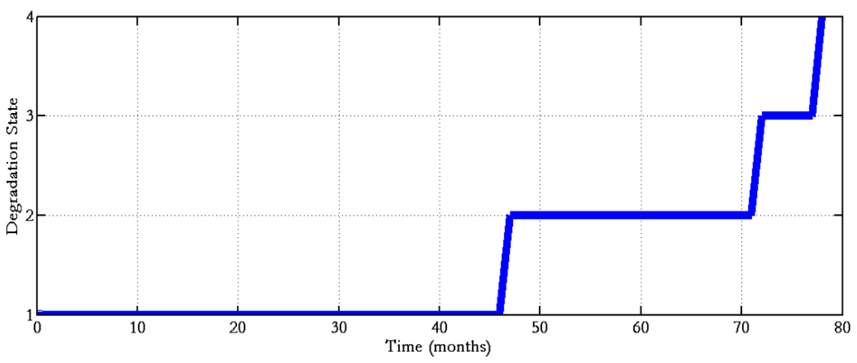
5.1. Degradation Trajectory Simulation

The CWRU bearing dataset did not contain the vibration signals measured during complete degradation trajectories—from normal condition to failure; it only included the vibration behavior for different bearings at different states of degradation. Thus, in order to include time dependence into the available dataset, we artificially generated $K=200$ bearing degradation trajectories $Z^k=\left\{Z_t^k,t=1,\dots ,l_k\right\}$ by Monte Carlo sampling of the sojourn times from the Weibull distributions with transition rate functions (see Appendix A for more details):

$${\lambda }_{i,i+1}\left(t\right)=\frac{{\beta }_{i,i+1}}{{\alpha }_{i,i+1}}{\left(\frac{t}{{\alpha }_{i,i+1}}\right)}^{{\beta }_{i,i+1}-1}{\alpha }_{i,i+1}>0,{\beta }_{i,i+1}>0,t\ge 0,i=1,\dots ,3$$

(11)

Without loss of generality, we arbitrarily set the value of parameters ${\alpha }_{i,i+1}$ and ${\beta }_{i.i+1}$, which are reported in

Table 3. Values of the scale parameters ${\alpha }_{i,i+1}$, shape parameters ${\beta }_{i,i+1}$ and expected sojourn time in each degradation state.

$\mathit{i}$	${\mathit{\alpha }}_{\mathit{i},\mathit{i}+1}$	${\mathit{\beta }}_{\mathit{i},\mathit{i}+1}$	Expected Sojourn Time (Month)
1	55	3.8	49.7083
2	33	4	29.9113
3	15	4.2	13.6341

.

Figure 3 shows an example of simulated degradation trajectory for a bearing.

Then, assuming the vibration signal is measured with a time interval, $\Delta$, equal to 1 month, thus allowing the classification of the bearing degradation state with the same frequency, we built artificial observation sequences ${\mathit{O}}^k=\left\{O_t^k,t=1,\dots ,l_k\right\}$, $k=1,\dots ,200$, by associating a KNN classification to the corresponding bearing true degradation state $Z_t^k$. This was done by Monte Carlo sampling of the KNN classification using the confusion matrix of Table 2, which refers to the performance of the KNN on the CWRU bearing dataset. For example, if we consider a bearing whose true degradation state is 1, the correct classification is sampled with a probability of 0.887, in states 2, 3, and 4 are 0.082, 0.031, and 0.000, respectively. Figure 4 shows the classifications of the degradation state obtained during the degradation trajectory of Figure 3. This is the input to the proposed hybrid ECS + HCTFSHSMM for on-line diagnostics of the bearing degradation state.

5.2. Results

The results of the application of the procedure introduced in Section 3, Section 4 and Section 5 to the bearings case study are presented and discussed in this subsection.

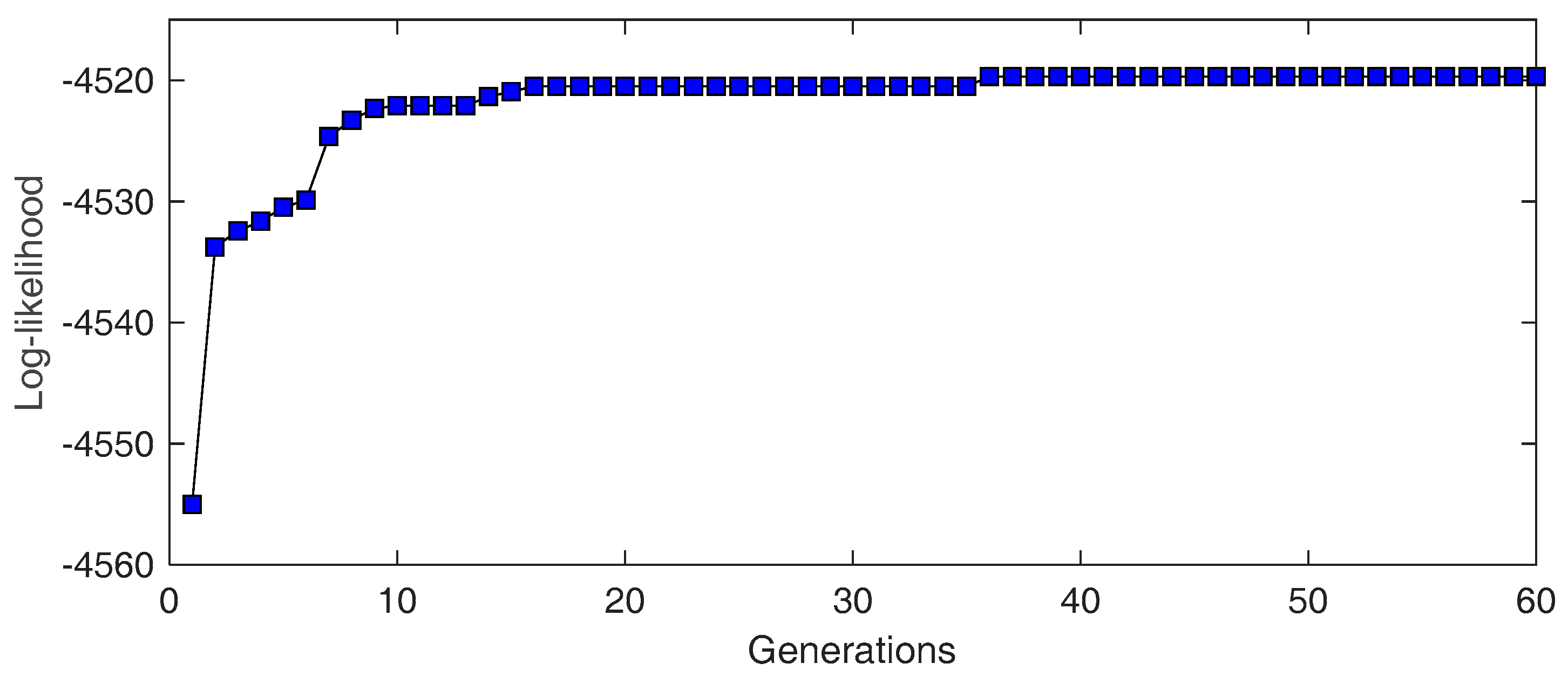
5.2.1. Parameter Optimization

To estimate the $C=6$ parameters of the model, $\mathit{\theta }=\left({\alpha }_{1,2},{\alpha }_{2,3},{\alpha }_{3,4},{\beta }_{1,2},{\beta }_{2,3},{\beta }_{3,4}\right)$, the MLE-based approach was applied. The objective function to be maximized is the log-likelihood in Equation (6), where the observation matrix $B$ is given in Table 2. Figure 5 shows the value of the log-likelihood of the best candidate solution in the current population at each iteration (also referred to as generation). After 36 iterations, there was no substantial improvement in the fitness function. This suggested that the algorithm had converged.

The values of the best candidate solutions ${\widehat{\vartheta }}_{opt}$ are reported in

Table 4. Maximum likelihood estimation (MLE) estimates of the parameters of the model using differential evolution (DE).

$\mathit{i}$	${\widehat{\mathit{\alpha }}}_{\mathit{i},\mathit{i}+1}$	${\widehat{\mathit{\beta }}}_{\mathit{i},\mathit{i}+1}$
1	54.7862	3.9610
2	31.5632	4.1578
3	13.7613	4.5585

.

Notice that they are very close to the parameters values used to generate the observation trajectories; specifically, $L^{*}\left({\widehat{\mathit{\vartheta }}}_{opt}\right)=-4519.7$, and $L^{*}\left({\mathit{\theta }}_{real}\right)=-4507.4$, and the difference $L^{*}\left({\widehat{\mathit{\vartheta }}}_{opt}\right)-L^{*}\left({\mathit{\theta }}_{real}\right)=12.3$ with a relative error of 0.27%.

With respect to the parameters values estimation,

Table 5. Relative percentage error for each estimated parameter.

$\mathit{i}$	$\frac{\widehat{|{\mathit{\alpha }}_{\mathit{i},\mathit{i}+1}}-{\mathit{\alpha }}_{\mathit{i},\mathit{i}+1}|}{{\mathit{\alpha }}_{\mathit{i},\mathit{i}+1}}\%$	$\frac{\widehat{|{\mathit{\beta }}_{\mathit{i},\mathit{i}+1}}-{\mathit{\beta }}_{\mathit{i},\mathit{i}+1}|}{{\mathit{\beta }}_{\mathit{i},\mathit{i}+1}}\%$
1	0.39%	4.24%
2	4.35%	3.94%
3	8.26%	8.54%

reports the relative percentage errors.

We found that the smaller the expected sojourn time in a state (see Table 3), the larger was the error in the parameter estimate. This can be attributed to the fact that the relevance of the censoring mechanism introduced by time discretization increases (see Section 3). Notice that increasing the number of observation sequences used to estimate MLEs of the parameters of the transition time distributions decreases the estimation error, according to the consistency property of MLE [43].

5.2.2. Assessment of the Degradation State

The MAP estimation introduced in Section 4 was applied to 200 other observation trajectories sampled by applying the same procedure described in Section 5.1. Figure 6 shows an example of observed trajectory (squares) and the corresponding estimated degradation state sequence (triangles) provided by the proposed methodology when it was applied at the end of the degradation trajectory (i.e., at $\tau =119$ months). It clearly emerges that this allows:

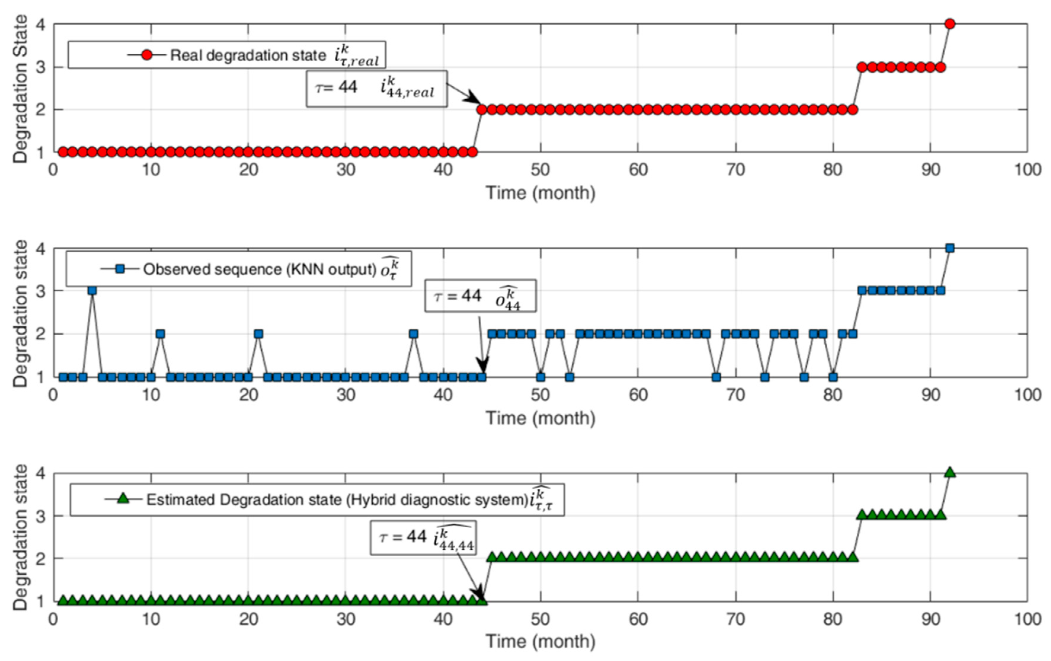
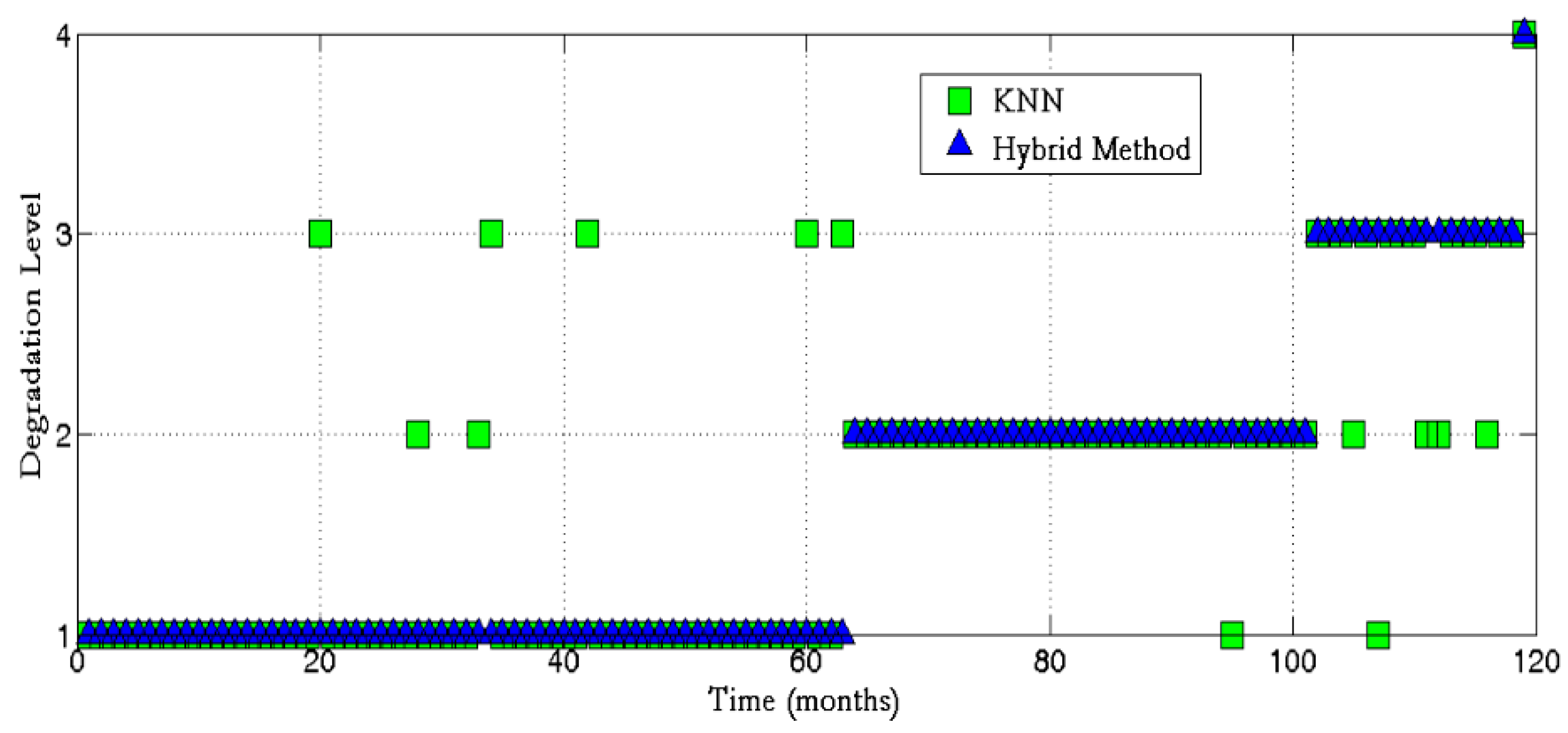
• Correction of the misclassifications of the KNN classifier. In particular, the decoded sequences are always increasing in monotone due to the fact that the underlying semi-Markov process allows only left-to-right transitions.
• Estimation, in an unambiguous way, of the time instant that the bearing entered for the first time in a given state. With reference to Figure 6, we can state that the bearing entered for the first time in states 2 and 3 at time instants 65 and 102 (months), respectively. Notice that this information cannot be retrieved by the KNN-based ECS only as it is pointwise static.

Table 6. Classification performance of the KNN classifier and the proposed hybrid method.

$\mathit{i}$	Mean Misclassification Rate	Maximum Misclassification Rate
KNN ($o_{\tau }^k)$	0.1195 ± 0.0338	0.2388
Hybrid Method (${\widehat{i}}_{\tau ,\tau }^k)$	0.0276 ± 0.0203	0.0960

reports the average misclassification rate value, which is defined as

$$\frac{1}{{\sum }_{k=1}^K{l}_k}{\sum }_{k=1}^K{\sum }_{\tau =1}^{l_k}{1}_{\{i_{\tau ,real}^k\ne {\widehat{i}}_{\tau ,\tau }^k\}}$$

(12)

where $i_{\tau ,real}^k$ is the true state of the bearing at time $\tau$ for the $k$-th sequence of observations, ${\widehat{i}}_{\tau ,\tau }^k$ the corresponding state estimated by the hybrid method at time $\tau$, using the observation sequence ${\mathit{O}}_{1:\tau }^k$. For comparison, the misclassification rate in Equation (12) was also computed considering the KNN classification algorithm, which is indicated by $o_{\tau }^k$, instead of ${\widehat{i}}_{\tau ,\tau }^k$ in (12) (Table 6).

Table 6 shows that the use of the hybrid method to estimate the degradation state significantly decreased the misclassification rate of the KNN classifier. Notice that errors in the estimation of the degradation state mainly occurred in correspondence to the jumping times from one state to the next degraded state. For example, consider Figure 7, which refers to the estimation of the sequence of states ${\widehat{i}}_{\tau ,\tau }^k$. Here, at time $\tau =44$, i.e., in the proximity of the real jumping time from state 1 towards state 2, $43<\tau \le 44,$ the hybrid method misclassifies the state as 1.

As time passes and new observations are collected, the hybrid method makes new estimates of the previous component state, i.e., at time $t>\tau$ it is possible to obtain a new classification ${\widehat{i}}_{\tau ,t}^k$ that considers the observation sequence $O_{1:t}^k$, and it is expected to be more accurate than ${\widehat{i}}_{\tau ,\tau }^k$, which is based on more information. For example, Figure 8 shows the estimate of the degradation state at time $\tau =44$ performed using the observation collected until time $t=\tau =44$ (top), $t=45$ (middle), and $t$ (bottom). Notice that at time $t=45$, the hybrid method is able to correctly classify the component state. This is a useful piece of information because the next transition depends on the sojourn time in this state. By contrast, the KNN does not correct the degradation state estimate based on the current knowledge of the degradation process.

5.2.3. Computational Time for On-Line Degradation State Assessment

With regards to the computational time, testing a signal of length $L^{sig}=2^{14}$ samples, as in Reference [22], requires: (1) the extraction of the features in Table 1; (2) the classification label provided by the one-stage KNN; and (3) correcting the classification provided by the KNN classifier through the proposed hybrid approach. On average, these three steps require 1.83 s using an Intel Core i7-7700 CPU @ 3.60 GHz processor with 8 GB RAM in MATLAB 2017b environment. Therefore the proposed approach is suitable for use in field operation.

6. Discussion and Outlooks

In this work, we considered a multistate degradation model that allows only left-to-right transitions to the neighbor state. However, different transition types can be considered in practice, such as direct transitions to the failure state (e.g., with respect to Figure 2, transitions from state 2 to state 4) or right-to-left transition due to preventive maintenance actions. The generalization of the proposed approach requires modeling more complex likelihood functions, although it does not impact the underlying structure of the approach.

A main limitation of our approach is that it assumes the availability of signal data for which the corresponding degradation state is known. Indeed, this information may not be available in many industrial applications. Future works will investigate the solution proposed by Cannarile et al. [19] to build an unsupervised clustering approach to identify the degradation state of the component. After this step, an ECS can be developed and combined with an HSMM as discussed in this work.

Finally, the developed approach estimates the parameters of the HSMM through an analytical solution to the problem of correcting the ECS output, which makes our hybrid method preferable to any other heuristic approach. However, this analytic approach is not applicable when the amount of data available is poor and the system is complex. In these cases, heuristics may be necessary for the approach to be applicable to real industrial settings. For example, the degradation state predicted at the previous time-step can be added as an additional feature to the diagnostic classifier. The integration of the proposed approach with heuristics will be addressed in future research work.

7. Conclusions

In this work, we have presented a novel diagnostic method for assessing the degradation state of industrial components in situations where the degradation process is not directly observable, but there is a classifier that provides an estimation of the actual state based on sensor signals. To improve the diagnostic performance, the classifier is integrated with a HCTFSSMM capturing the dynamic evolution of the degradation process. The resulting HCTFSHSMM parameters (transition function rates) are estimated using a method based on advanced MLE combined with the DE optimization technique.

The HCTFSHSMM adjusts the classifications provided by the empirical classifier ECS, by exploiting the knowledge of the sequence of observations collected from the monitored component. Thus, the final classification performance outperforms that of a single stage empirical classifier. This is shown by the considered case study of bearing degradation described by Weibull-distributed state sojourn times. Furthermore, the proposed approach can be used to fully characterize the underlying semi-Markov process as we can estimate both the current state and the time instant the system entered it, which is not possible using only the ECS.

References

1. Baraldi, P.; Compare, M.; Zio, E. A practical analysis of the degradation of a nuclear component with field data. In Reliability and Risk Analysis: Beyond the Horizon; Steenbergen, R.D.J.M., van Gelder, P.H.A.J.M., Miraglia, S., Vrouwenvelder, A.C.W.M., Eds.; CRC Press: Boca Raton, FL, USA, 2013. [Google Scholar]
2. Giorgio, M.; Guida, M.; Pulcini, G. An age- and state-dependent Markov model for degradation processes. IIE Trans. 2011, 43, 621–632. [Google Scholar] [CrossRef]
3. Moghaddass, R.; Zuo, M.J. A parameter estimation method for a condition-monitored device under multistate deterioration. Reliab. Eng. Syst. Saf. 2012, 106, 94–103. [Google Scholar] [CrossRef]
4. Vrignat, P.; Avila, M.; Duculty, F.; Aupetit, S.; Slimane, M.; Kratz, F. Maintenance policy: Degradation laws versus Hidden Markov Model availability indicator. Proc. Inst. Mech. Eng. Part O J. Risk Reliab. 2011, 226, 137–155. [Google Scholar] [CrossRef]
5. Lemaitre, J. A Course on Damage Mechanics; Springer: Berlin/Heidelberg, Germany, 1992. [Google Scholar]
6. Grall, A.; Blain, C.; Barros, A.; Lefebvre, Y.; Billy, F. Modeling of Stress Corrosion Cracking with Periodic Inspection. In Proceeding of the 32nd ESReDA Seminar on Italy Maintenance Modeling and Application, Alghero, Italy, 8–9 May 2007; Volume 1, pp. 253–260. [Google Scholar]
7. Baraldi, P.; Compare, M.; Despujols, A.; Zio, E. Modelling the effects of maintenance on the degradation of a water-feeding turbo-pump of a nuclear power plant. Proc. Inst. Mech. Eng. Part O J. Risk Reliab. 2011, 225, 169–183. [Google Scholar] [CrossRef] [Green Version]
8. Compare, M.; Legnani, L.; Zio, E. MUSTADEPT: A tool for the analysis of industrial equipment degradation Safety and Reliability: Methodology and Applications. In Proceedings of the European Safety and Reliability Conference (ESREL 2014), Tri City, Poland, 27–30 June 2014; pp. 873–881. [Google Scholar]
9. Baraldi, P.; Balestrero, A.; Compare, M.; Benetrix, L.; Despujols, A.; Zio, E. A modeling framework for maintenance optimization of electrical components based on fuzzy logic and effective age. Qual. Reliab. Eng. Int. 2013, 29, 385–405. [Google Scholar] [CrossRef]
10. Baraldi, P.; Compare, M.; Zio, E. Uncertainty analysis in degradation modeling for maintenance policy assessment. Proc. Inst. Mech. Eng. Part O J. Risk Reliab. 2013, 22, 267–278. [Google Scholar] [CrossRef]
11. Giorgio, M.; Guida, M.; Pulcini, G. A state-dependent wear model with an application to marine engine cylinder liners. Technometrics 2010, 52, 172–187. [Google Scholar] [CrossRef]
12. Cannarile, F.; Compare, M.; Rossi, E.; Zio, E. A fuzzy expectation maximization based method for estimating the parameters of a multi-state degradation model from imprecise maintenance outcomes. Ann. Nucl. Energy 2017, 110, 739–752. [Google Scholar] [CrossRef] [Green Version]
13. Kwan, C.; Zhang, X.; Xu, R.; Haynes, L. A novel approach to fault diagnostics and prognostics. In Proceedings of the IEEE International Conference on Robotics and Automation, Taipei, Taiwan, 14–19 September 2003; Volume 1, pp. 604–609. [Google Scholar]
14. Rabiner, L.R. A tutorial on hidden Markov models and selected applications in speech recognition. Proc. IEEE 1989, 77, 257–286. [Google Scholar] [CrossRef] [Green Version]
15. Moghaddass, R.; Zuo, M.J. An integrated framework for online diagnostic and prognostic health monitoring using a multistate deterioration process. Reliab. Eng. Syst. Saf. 2014, 124, 92–104. [Google Scholar] [CrossRef]
16. Kohavi, R.; John, G.H. Wrappers for feature subset selection. Artif. Intell. 1997, 97, 273–324. [Google Scholar] [CrossRef]
17. Ocak, H.; Loparo, K.A.; Discenzo, F.M. Online tracking of bearing wear using wavelet packet decomposition and probabilistic modeling: A method for bearing prognostics. J. Sound Vib. 2007, 302, 951–961. [Google Scholar] [CrossRef]
18. Georgoulas, G.; Loutas, T.; Stylios, C.D.; Kostopoulos, V. Bearing fault detection based on hybrid ensemble detector and empirical mode decomposition. Mech. Syst. Signal Process. 2013, 41, 510–525. [Google Scholar] [CrossRef]
19. Cannarile, F.; Baraldi, P.; Compare, M.; Borghi, D.; Capelli, L.; Cocconcelli, M.; Lahrache, A.; Zio, E. An unsupervised clustering method for assessing the degradation state of cutting tools in the packaging industry. In Safety and Reliability: Theory and Application, Proceedings of the European Safety and Reliability Conference (ESREL 2017), Portoroz, Slovenia, 18–22 June 2017; CRC Press: Boca Raton, FL, USA, 2017. [Google Scholar]
20. Medjaher, K.; Tobon-Mejia, D.A.; Zerhouni, N. Remaining useful life estimation of critical components with application to bearings. IEEE Trans. Reliab. 2012, 61, 292–302. [Google Scholar] [CrossRef] [Green Version]
21. Dong, M.; He, D.A. Hidden semi-Markov model-based methodology for multi-sensor equipment health diagnosis and prognosis. Eur. J. Oper. Res. 2007, 178, 858–878. [Google Scholar] [CrossRef]
22. Baraldi, P.; Cannarile, F.; Di Maio, F.; Zio, E. Hierarchical k-nearest neighbours classification and binary differential evolution for fault diagnostics of automotive bearings operating under variable conditions. Eng. Appl. Artif. Intell. 2016, 56, 1–13. [Google Scholar] [CrossRef] [Green Version]
23. Narasimhan, S.; Roychoudhury, I.; Balaban, E.; Saxena, A. Combining model-based and feature-driven approaches: A case study on electromechanical actuators. In Proceedings of the 21st International Workshop on Principles of Diagnosis, Portland, OR, USA, 13–16 October 2010. [Google Scholar]
24. Caesarendra, W.; Tjahwowidodo, T. A review of feature extraction methods in vibration-based condition monitoring and its application for degradation trend estimation of low-speed slew bearing. Machines 2017, 5, 21. [Google Scholar] [CrossRef]
25. Cannarile, F.; Compare, M.; Zio, E. A Fault Diagnostic tool based on a First Principle Model Simulator. In Model-Based Safety and Assessment, IMBSA 2017; Lecture Notes in Computer Science (Including Subseries Lecture Notes in Artificial Intelligence and Lecture Notes in Bioinformatics); Bozzano, M., Papadopoulos, Y., Eds.; Springer: Cham, Switzerland, 2017; Volume 10437, pp. 179–193. [Google Scholar]
26. Baraldi, P.; Pedroni, N.; Zio, E. Application of a niched Pareto genetic algorithm for selecting features for nuclear transients classification. Int. J. Intell. Syst. 2009, 24, 118–151. [Google Scholar] [CrossRef]
27. Cordón, O.; Herrera-Viedma, E.; Luque, M. Improving the learning of Boolean queries by means of a multiobjective IQBE evolutionary algorithm. Inf. Process. Manag. 2006, 42, 615–632. [Google Scholar] [CrossRef] [Green Version]
28. He, X.; Zhang, Q.; Sun, N.; Dong, Y. Feature selection with discrete binary differential evolution. In Proceedings of the 2009 International Conference on Artificial Intelligence and Computational Intelligence (AICI 2009), Shanghai, China, 7–8 November 2019; Volume 4, pp. 327–330. [Google Scholar]
29. Tušar, T.; Filipič, B. Differential evolution versus genetic algorithms in multiobjective optimization. In Evolutionary Multi-criterion Optimization, EMO 2007; Lecture Notes in Computer Science (Including Subseries Lecture Notes in Artificial Intelligence and Lecture Notes in Bioinformatics); Obayashi, S., Deb, K., Poloni, C., Hiroyasu, T., Murata, T., Eds.; Springer: Berlin/Heidelberg, Germany, 2007. [Google Scholar]
30. Deb, K.; Pratap, A.; Agarwal, S.; Meyarivan, T. A fast and elitist multiobjective genetic algorithm: NSGA-II. IEEE Trans. Evol. Comput. 2002, 6, 182–197. [Google Scholar] [CrossRef] [Green Version]
31. Zitzler, E.; Laumanns, M.; Thiele, L. SPEA2: Improving the Performance of the Strength Pareto Evolutionary Algorithm; Technical Report 103; Computer Engineering and Communication Networks Lab (TIK), Swiss Federal Institute of Technology (ETH): Zurich, Switzerland, 2001. [Google Scholar]
32. Zitzler, E.; Künzli, S. Indicator-based selection in multi-objective search. In Parallel Problem Solving fron Nature-PPSN VIII; Lecture Notes in Computer Science (Including Subseries Lecture Notes in Artificial Intelligence and Lecture Notes in Bioinformatics); Yao, X., Burke, E.K., Lozano, J.A., Smith, J., Merelo-Guervós, J.J., Bullinaria, J.A., Rowe, J.E., Kabán, P.T., Schwefel, H., Eds.; Springer: Berlin/Heidelberg, Germany, 2004. [Google Scholar]
33. Altman, N.S. An introduction to kernel and nearest-neighbor nonparametric regression. Am. Stat. 1992, 46, 175–185. [Google Scholar]
34. Bang, S.L.; Yang, J.D.; Yang, H.J. Hierarchical document categorization with k-NN and concept-based thesauri. Inf. Process. Manag. 2006, 42, 387–406. [Google Scholar] [CrossRef]
35. Wu, W.F.; Ni, C.C. A study of stochastic fatigue crack growth modeling through experimental data. Probab. Eng. Mech. 2003, 18, 107–118. [Google Scholar] [CrossRef]
36. Boutros, T.; Liang, M. Detection and diagnosis of bearing and cutting tool faults using hidden Markov models. Mech. Syst. Signal Process. 2011, 25, 2102–2124. [Google Scholar] [CrossRef]
37. Baum, L.E.; Petrie, T. Statistical Inference for Probabilistic Functions of Finite State Markov Chains. Ann. Math. Stat. 1966, 37, 1554–1563. [Google Scholar] [CrossRef]
38. Baum, L.E.; Eagon, J.A. An inequality with applications to statistical estimation for probabilistic functions of Markov processes and to a model for ecology. Bull. Am. Math. Soc. 1967, 73, 360–363. [Google Scholar] [CrossRef]
39. Baum, L.E.; Petrie, T.; Soules, G.; Weiss, N. A Maximization Technique Occurring in the Statistical Analysis of Probabilistic Functions of Markov Chains. Ann. Math. Stat. 1970, 41, 164–171. [Google Scholar] [CrossRef]
40. Barbu, V.S.; Limnios, N. Semi-Markov Chains and Hidden Semi-Markov Models towards Applications in Reliability and DNA Analysis; Lecture notes in Statistics; Springer: New York, NY, USA, 2008; Volume 191. [Google Scholar]
41. Moghaddass, R.; Zuo, M.J.; Zhao, X. Modeling multi-state equipment degradation with non-homogeneous continuous-time hidden semi-markov process. In Diagnostics and Prognostics of Engineering Systems: Methods and Techniques; IGI Global: Hershey, PA, USA, 2012; pp. 51–181. [Google Scholar]
42. Storn, R.; Price, K. Differential Evolution—A Simple and Efficient Heuristic for Global Optimization over Continuous Spaces. J. Glob. Optim. 1997, 11, 341–359. [Google Scholar] [CrossRef]
43. Zio, E. An Introduction to the Basics of Reliability and Risk Analysis; World Scientific Publishing Company: Singapore, 2007. [Google Scholar]
44. Yu, S.-Z. Hidden semi-Markov models. Artif. Intell. 2010, 174, 215–243. [Google Scholar] [CrossRef]
45. O’Donnell, P.; Bell, R.N.; McWilliams, D.W.; Singh, C.; Wells, S.J. Report of large motor reliability survey of industrial and commercial installations. In Proceedings of the IEEE Conference Record of Industrial and Commercial Power Systems Technical Conference, Philadelphia, PA, USA, 10–13 May 1983; pp. 58–70. [Google Scholar]
46. Jiang, L.; Xuan, J.; Shi, T. Feature extraction based on semi-supervised kernel Marginal Fisher analysis and its application in bearing fault diagnosis. Mech. Syst. Signal Process. 2013, 41, 113–126. [Google Scholar] [CrossRef]
47. Zhang, Y.; Zuo, H.; Bai, F. Classification of fault location and performance degradation of a roller bearing. Measurement 2013, 46, 1178–1189. [Google Scholar] [CrossRef]
48. Zhu, K.; Song, X.; Xue, D. A roller bearing fault diagnosis method based on hierarchical entropy and support vector machine with particle swarm optimization algorithm. Measurement 2014, 47, 669–675. [Google Scholar] [CrossRef]
49. Caesarendra, W.; Tjahjowidodo, T.; Kosasih, B.; Tieu, A.K. Integrated condition monitoring and prognosis method for incipient defect detection and remaining life prediction of low speed slew bearing. Machines 2017, 5, 11. [Google Scholar] [CrossRef]
50. Alwadie, A. The decision making system for condition monitoring of induction motors based on vector control model. Machines 2018, 5, 27. [Google Scholar] [CrossRef]
51. Tobon-Mejia, D.A.; Medjaher, K.; Zerhouni, N.; Tripot, G. A data-driven failure prognostics method based on mixture of gaussians hidden markov models. IEEE Trans. Reliab. 2012, 61, 491–503. [Google Scholar] [CrossRef] [Green Version]
52. Soualhi, A.; Razik, H.; Clerc, G.; Doan, D.D. Prognosis of bearing failures using hidden markov models and the adaptive neuro-fuzzy inference system. IEEE Trans. Ind. Electron. 2014, 61, 2864–2874. [Google Scholar] [CrossRef]
53. Ioannides, E.; Harris, T.A. A new fatigue life model for rolling bearings. J. Tribol. 1985, 107, 367–377. [Google Scholar] [CrossRef]
54. Case Western Reserve University Bearing Data Center Website. Available online: http://csegroups.case.edu/bearingdatacenter/pages/welcome-case-western-reserve-university-bearing-data-center-website (accessed on 20 January 2018).
55. Pak, A.; Parham, G.A.; Saraj, M. Inference for the Weibull distribution based on fuzzy data. Rev. Colomb. Estad. 2013, 36, 339–358. [Google Scholar]
56. Sokolova, M.; Lapalme, G. A systematic analysis of performance measures for classification tasks. Inf. Process. Manag. 2009, 45, 427–437. [Google Scholar] [CrossRef]
57. Limnios, N.; Oprisan, G. Semi-Markov Processes and Reliability; Birkhauser: Boston, MA, USA, 2001. [Google Scholar]
Figure 1. The hybrid diagnostic system based on homogeneous continuous-time finite-state hidden semi-Markov (HCTFSHSMM). In particular, we set the entries of the observation matrix B as the estimated misclassification probabilities of the KNN classification algorithm.
Machines 06 00034 g001
Figure 2. Four-state (left-to-right) model for the degrading bearing.
Machines 06 00034 g002
Figure 3. Example of simulated degradation trajectory.
Machines 06 00034 g003
Figure 4. Classification of the degradation state during the degradation trajectory of Figure 3. The true degradation state of the component is state 1: from to 46, state 2: from 46 to 71, state 3: from 72 to 77, and state 4: at time 78.
Machines 06 00034 g004
Figure 5. Log-likelihood value of the best individual in the population at successive generations.
Machines 06 00034 g005
Figure 6. Example of observed sequence (squares) and estimated degradation state sequence (triangle). The true degradation state of the component is state 1: up to time 64 months, state 2: from time 65 to time 101 months, state 3: from time 102 to time 118 months, and state 4: at time 119 months.
Machines 06 00034 g006
Figure 7. Typical case in which degradation state errors occur (Top: real degradation states; middle: degradation states estimated by the KNN classifier; bottom: degradation states estimated by the hybrid diagnostic system).
Machines 06 00034 g007
Figure 8. Estimate of the degradation state at time τ = 44 performed using the observation collected until time t = τ = 44 (top), t = 45 (middle), and t = 46 (bottom). Notice that at time t = 45 , the hybrid method is able to correctly classify the component state.
Machines 06 00034 g008