Study on Payload Effects on the Joint Motion Accuracy of Serial Mechanical Mechanisms

Abstract

Robotic manipulators have been widely used in many arenas, when the robotic arm performs positioning, a traditional controller (e.g., a proportional-integral-derivative, PID controller) has the problem of not being able to compensate the payload variations. When the end-effector of the robotic arm grasps different payload masses as most applications require, the output of joint motion will vary under different payload masses, which will decrease the end-effector positioning accuracy of the robotic arm system. Based on the model reference adaptive control technique, the payload variation effect can be solved, therefore improving the positioning accuracy. This paper studies payload effects on the joint motion accuracy of serial mechanical mechanisms.

1. Introduction

Proportional-integral-derivative (PID) control is a widely used control method in many industries. For example, in many industries using robotic arms, PID control applies to each joint to control the whole robotic arm. By adjusting the PID gains of the PID controller, one can have the desired output performance. In [1], a discrete PID controller was designed for use in nano scale systems. In [2], a PID controller with additional imposed nonlinear logic was reviewed for robot motion positioning control. In [3], control strategies that implement planar micro assembly using groups of stress-engineered MEMS micro robots controlled through a single global control signal were presented. Model reference adaptive control (MRAC) is another control method that was proposed early on by Landau [4], and it has since been developed [5,6,7,8]. In [9], the implementation of MRAC to a dynamically unknown hydraulic robot for position tracking was presented. A recursive parameter estimator was employed for the parameter estimation in the MRAC system. The hydraulic robot was tested for a step input signal change, and it was found that the MRAC can provide better tracking than that of the PID controller, and the MRAC is sufficient enough to replace the classical PID controller. However, a minor problem was discovered, in that there is a small oscillation at the beginning of the motion when MRAC is applied. In [10], the study presented the application of a MRAC composite system used for tracking the endpoint of a flexible joint manipulator used in space. In [11], a model reference tracking-based adaptive PID controller was designed by inserting a PID controller to the feedback path for robot motion control, and the control system allows one to manipulate motions of an unstable robot. The reason that one needs to apply the adaptive control—especially the model reference adaptive control approach—is that traditional controllers cannot compensate the payload variations. When the end-effector grasps different payload masses, the joint output will vary under different payload masses, which will affect the positioning accuracy of the end-effector. Whereas for the model reference adaptive control, the above problem can be effectively resolved, and payload variation effect can be compensated. The MRAC (model reference adaptive control) technique was first proposed by Whitaker [12] in 1958, when he examined the adaptive flight control system, employing a reference model to produce the difference between the real and expected behavior. The difference was employed to adjust the parameters of the control system in order to obtain the expected outcome, regardless of some uncertainties and changing dynamics. The MRAC was later developed further. Dubowsky [5] was the first to apply the MRAC in a robotic manipulator. A linear time-invariant differential equation was employed as a reference model for every single joint in the robotic arm. The robotic arm was manipulated by tuning the gains of the position and velocity feedback system to track the model. The author employed the steepest-descent approach for renewing the feedback system gains, after which Horowitz applied the hyper-stability method and developed an adaptive algorithm [13] for a mechanical system, with the aim of compensating a nonlinear term in the dynamic equation and decoupling the existing interactions between the each joint of the robotic system. The MRAC proposed by Horowitz, and later associated developments by other authors, contains an adaptive algorithm block and a position feedback loop which provides the difference between desired and actual position of the joints. This difference is acted upon by the integral portion of a seemingly PID control structure before feedback values of position and velocity are subtracted from it. The problem associated with using a PID controller of not being able to compensate the payload variation is illustrated, and the general theory of model reference control is presented in the following section.

2. Payload Variation Effect and Model Reference Control

2.1. Two-Degrees of Freedom (DOF) Link Case

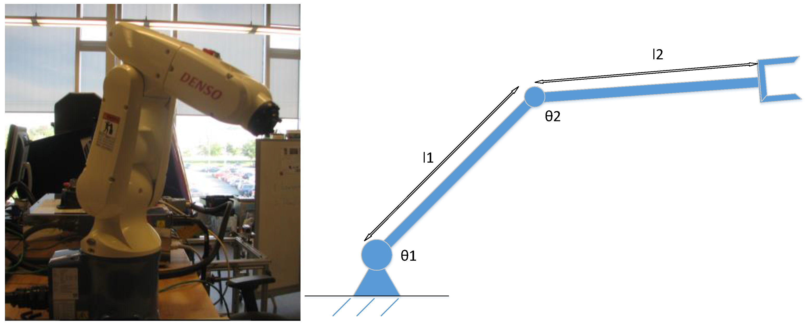
In order to implement PID control of the two-DOF (degrees of freedom) link manipulator case, as shown in Figure 1, the dynamic equation has to be derived. Here, by using the Lagrange method, the torques applied to the joints are determined:

$${\tau }_1=\frac{d}{dt}\frac{\partial L}{\partial \stackrel{•}{{\theta }_1}}-\frac{\partial L}{\partial {\theta }_1},{\tau }_2=\frac{d}{dt}\frac{\partial L}{\partial \stackrel{•}{{\theta }_2}}-\frac{\partial L}{\partial {\theta }_2}$$

(1)

The kinetic energy and potential energy for link 1 are expressed as:

$$K_1=\frac{1}{2}{m}_1{(l_1\stackrel{•}{{\theta }_1})}^2,P_1=m_{1}g(l_1\sin {\theta }_1)$$

(2)

where $m_1$ is the mass of link 1 and $m_2$ is the mass of link 2. For link 2, first write down the coordinates of the end of link 2, then differentiate them with respect to time in order to obtain the kinetic energy. Denote the Cartesian coordinates of the end of link 2 as (x₂, y₂).

$$x_2=l_1\cos {\theta }_1+l_2\cos ({\theta }_1+{\theta }_2),y_2=l_1\sin {\theta }_1+l_2\sin ({\theta }_1+{\theta }_2)$$

(3)

Differentiate with respect to time results in:

$$\stackrel{•}{x_2}=-l_1\stackrel{•}{{\theta }_1}\sin {\theta }_1-l_2(\stackrel{•}{{\theta }_1}+\stackrel{•}{{\theta }_2})\sin ({\theta }_1+{\theta }_2),\stackrel{•}{y_2}=l_1\stackrel{•}{{\theta }_1}\cos {\theta }_1+l_2(\stackrel{•}{{\theta }_1}+\stackrel{•}{{\theta }_2})\cos ({\theta }_1+{\theta }_2)$$

Therefore, the kinetic energy for link 2 is expressed as:

$$K_2=\frac{1}{2}{m}_2{v_2}^2=\frac{1}{2}{m}_2{l_1}^2{\stackrel{•}{{\theta }_1}}^2+\frac{1}{2}{m}_2{l_2}^2{(\stackrel{•}{{\theta }_1}+\stackrel{•}{{\theta }_2})}^2+m_2{l}_1{l}_2\cos {\theta }_2\stackrel{•}{{\theta }_1}(\stackrel{•}{{\theta }_1}+\stackrel{•}{{\theta }_2})$$

(4)

where ${v_2}^2={\stackrel{•}{x_2}}^2+{\stackrel{•}{y_2}}^2$.

The potential energy for link 2 is expressed as:

$$P_2=m_{2}g{l}_1\sin {\theta }_1+m_{2}g{l}_2\sin ({\theta }_1+{\theta }_2)$$

(5)

The total kinetic and potential energy are expressed as:

$$\begin{gathered} P=P_1+P_2=(m_1+m_2)g{l}_1\sin {\theta }_1+m_{2}g{l}_2\sin ({\theta }_1+{\theta }_2) \\ K=K_1+K_2=\frac{1}{2}(m_1+m_2){l_1}^2{\stackrel{•}{{\theta }_1}}^2+\frac{1}{2}{m}_2{l_2}^2{(\stackrel{•}{{\theta }_1}+\stackrel{•}{{\theta }_2})}^2+m_2{l}_1{l}_2\cos {\theta }_2\stackrel{•}{{\theta }_1}(\stackrel{•}{{\theta }_1}+\stackrel{•}{{\theta }_2}). \end{gathered}$$

The Lagrange is obtained as:

$$\begin{array}{l}L=K-P=\frac{1}{2}(m_1+m_2){l_1}^2{\stackrel{•}{{\theta }_1}}^2+\frac{1}{2}{m}_2{l_2}^2{(\stackrel{•}{{\theta }_1}+\stackrel{•}{{\theta }_2})}^2+m_2{l}_1{l}_2\cos {\theta }_2\stackrel{•}{{\theta }_1}(\stackrel{•}{{\theta }_1}+\stackrel{•}{{\theta }_2})\\ -(m_1+m_2)g{l}_1\sin {\theta }_1-m_{2}g{l}_2\sin ({\theta }_1+{\theta }_2)\end{array}$$

(6)

$$\begin{array}{cc}\hfill {\tau }_1& =\frac{d}{dt}\frac{\partial L}{\partial \stackrel{•}{{\theta }_1}}-\frac{\partial L}{\partial {\theta }_1}\hfill \\ & =((m_1+m_2){l_1}^2+m_2{l_2}^2+2m_2{l}_1{l}_2\cos {\theta }_2)\stackrel{••}{{\theta }_1}+(m_2{l_2}^2+m_2{l}_1{l}_2\cos {\theta }_2)\stackrel{••}{{\theta }_2}\hfill \\ & +(-2m_2{l}_1{l}_2\sin {\theta }_2)\stackrel{•}{{\theta }_1}\stackrel{•}{{\theta }_2}+(-m_2{l}_1{l}_2\sin {\theta }_2){\stackrel{•}{{\theta }_2}}^2+((m_1+m_2)l_1\cos {\theta }_1+m_2{l}_2\cos ({\theta }_1+{\theta }_2))g\hfill \end{array}$$

$$\begin{array}{cc}\hfill {\tau }_2& =\frac{d}{dt}\frac{\partial L}{\partial \stackrel{•}{{\theta }_2}}-\frac{\partial L}{\partial {\theta }_2}\hfill \\ & =(m_2{l_2}^2+m_2{l}_1{l}_2\cos {\theta }_2)\stackrel{••}{{\theta }_1}+(m_2{l_2}^2)\stackrel{••}{{\theta }_2}+(m_2{l}_1{l}_2\sin {\theta }_2){\stackrel{•}{{\theta }_1}}^2+m_2{l}_2\cos ({\theta }_1+{\theta }_2)g\hfill \end{array}$$

Putting them in a matrix form, we can obtain the following:

$$\left[\begin{array}{l}{\tau }_1\\ {\tau }_2\end{array}\right]=M\stackrel{••}{\theta }+N+Gg=\left[\begin{array}{cc}{m}_{11}& m_{12}\\ m_{12}& m_{22}\end{array}\right]\left[\begin{array}{l}\stackrel{••}{{\theta }_1}\\ \stackrel{••}{{\theta }_2}\end{array}\right]+\left[\begin{array}{l}{n}_{11}\\ n_{21}\end{array}\right]+\left[\begin{array}{l}{g}_{11}\\ g_{21}\end{array}\right]g$$

where $m_{11}=(m_1+m_2){l_1}^2+m_2{l_2}^2+2m_2{l}_1{l}_2\cos {\theta }_2$, $m_{12}=m_2{l_2}^2+m_2{l}_1{l}_2\cos {\theta }_2$, $m_{22}=m_2{l_2}^2$, $n_{11}=2(-m_2{l}_1{l}_2\sin {\theta }_2)\stackrel{•}{{\theta }_1}\stackrel{•}{{\theta }_2}+(-m_2{l}_1{l}_2\sin {\theta }_2){\stackrel{•}{{\theta }_2}}^2$, $n_{21}=m_2{l}_1{l}_2\sin {\theta }_2{\stackrel{•}{{\theta }_1}}^2$.

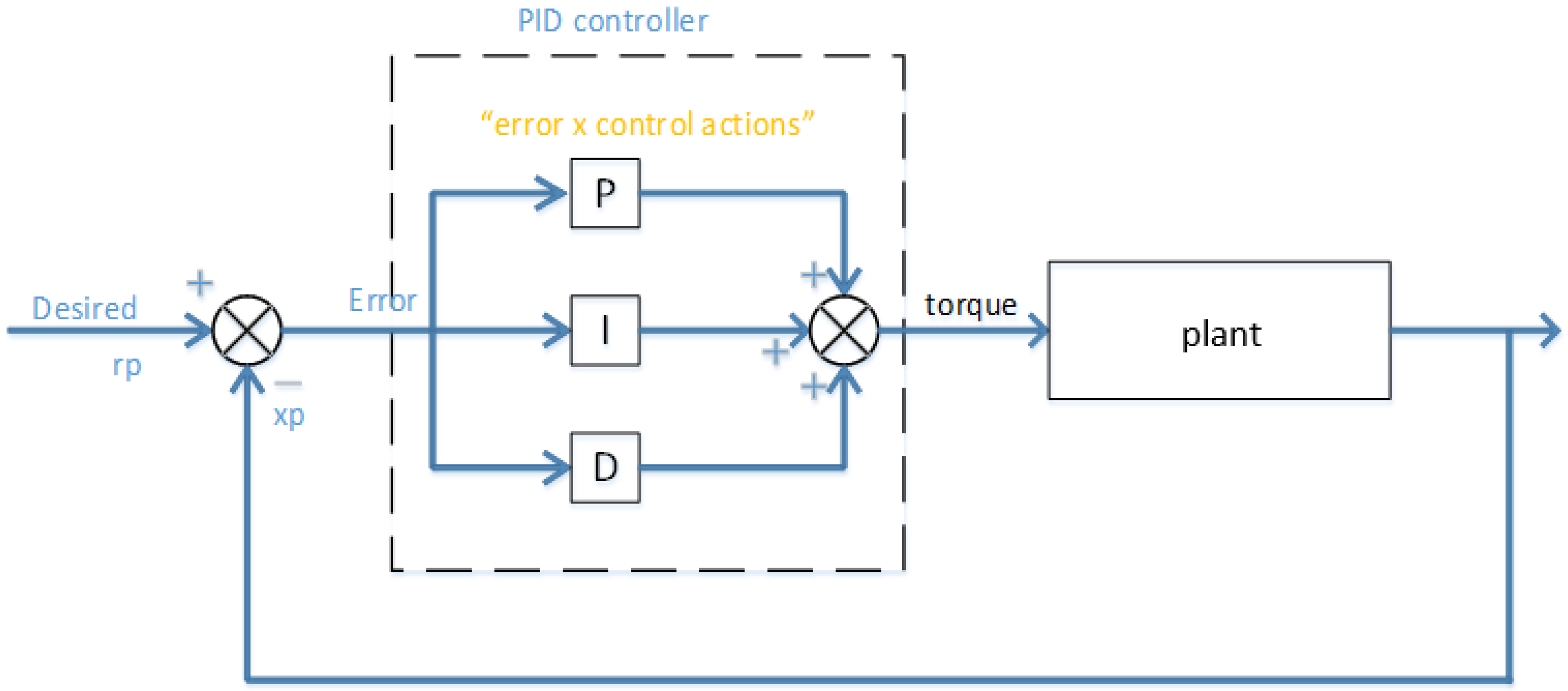
Now apply the PID controller, as shown in Figure 2, the plant’s output compares with the reference model, which generates a difference. This difference goes via the PID operation (i.e., through “error times control actions”). The output from the PID operation goes to the plant model’s input, and this circle keeps going, up to the point where the difference among the real plant’s output and the ideal one approaches zero. The controller output is the torque; i.e.,

$$K_{p}e+K_i{\displaystyle \int e}dt+K_d\stackrel{•}{e}=\left[\begin{array}{l}{\tau }_1\\ {\tau }_2\end{array}\right]$$

(7)

where error $e=r_p-x_p$. We know the two-link manipulator M and N matrices, the output from the manipulator (i.e., acceleration of joints 1 and 2) can be determined as follows:

$$\left[\begin{array}{l}{\tau }_1\\ {\tau }_2\end{array}\right]=M\stackrel{••}{\theta }+N+Gg=\left[\begin{array}{cc}{m}_{11}& m_{12}\\ m_{12}& m_{22}\end{array}\right]\left[\begin{array}{l}\stackrel{••}{{\theta }_1}\\ \stackrel{••}{{\theta }_2}\end{array}\right]+\left[\begin{array}{l}{n}_{11}\\ n_{21}\end{array}\right]+\left[\begin{array}{l}{g}_{11}\\ g_{21}\end{array}\right]g.$$

So $K_{p}e+K_i{\displaystyle \int e}dt+K_d\stackrel{•}{e}=\left[\begin{array}{l}{\tau }_1\\ {\tau }_2\end{array}\right]=M\stackrel{••}{\theta }+N+Gg$

$$\Rightarrow \left[\begin{array}{l}\stackrel{••}{{\theta }_1}\\ \stackrel{••}{{\theta }_2}\end{array}\right]=M^{-1}(K_{p}e+K_i{\displaystyle \int e}dt+K_d\stackrel{•}{e}-N)$$

(8)

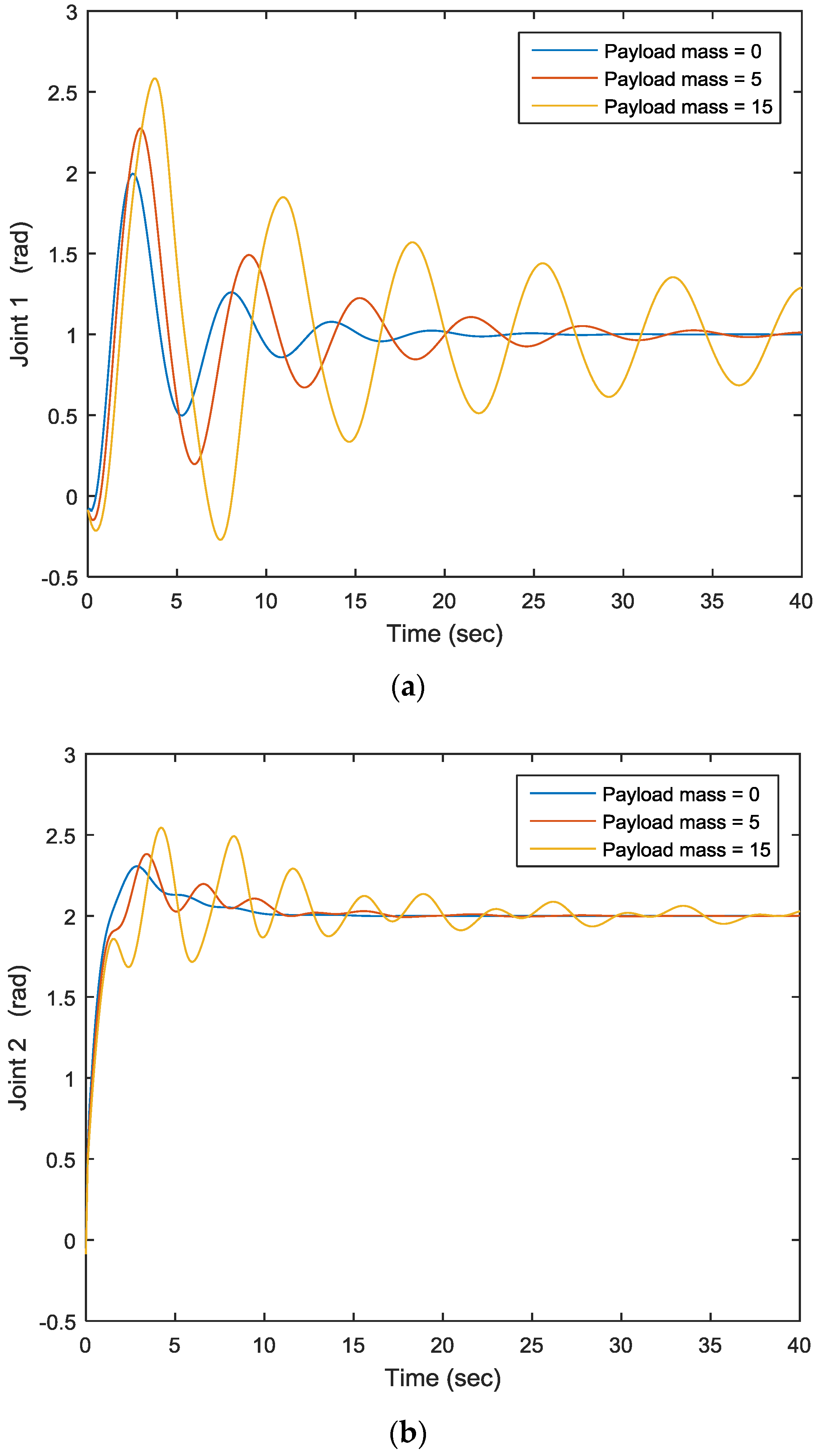
After deriving the acceleration of joints 1 and 2, take the time integral to obtain the velocity of joints 1 and 2, and take another integral to obtain the positon of joints 1 and 2.

$$\left[\begin{array}{l}\stackrel{•}{{\theta }_1}\\ \stackrel{•}{{\theta }_2}\end{array}\right]={\displaystyle \int \left[\begin{array}{l}\stackrel{••}{{\theta }_1}\\ \stackrel{••}{{\theta }_2}\end{array}\right]}dt,\left[\begin{array}{l}{\theta }_1\\ {\theta }_2\end{array}\right]={\displaystyle \int \left[\begin{array}{l}\stackrel{•}{{\theta }_1}\\ \stackrel{•}{{\theta }_2}\end{array}\right]}dt$$

(9)

After applying different payload masses, the joints’ motion outputs are illustrated in Figure 3. For joint 1, when the payload is 0, joint one’s motion is quite steady; however, when the payload increases to 5 and 15, one can see that joint 1’s motion is no longer the same, and the joint output is also going up and down, as shown in Figure 3. The same applies to joint 2. The output of joint motion varies, which decreases the end-effector positioning accuracy of the robotic arm system. In order to address the above problem, model reference control is applied to compensate the payload variation effect. 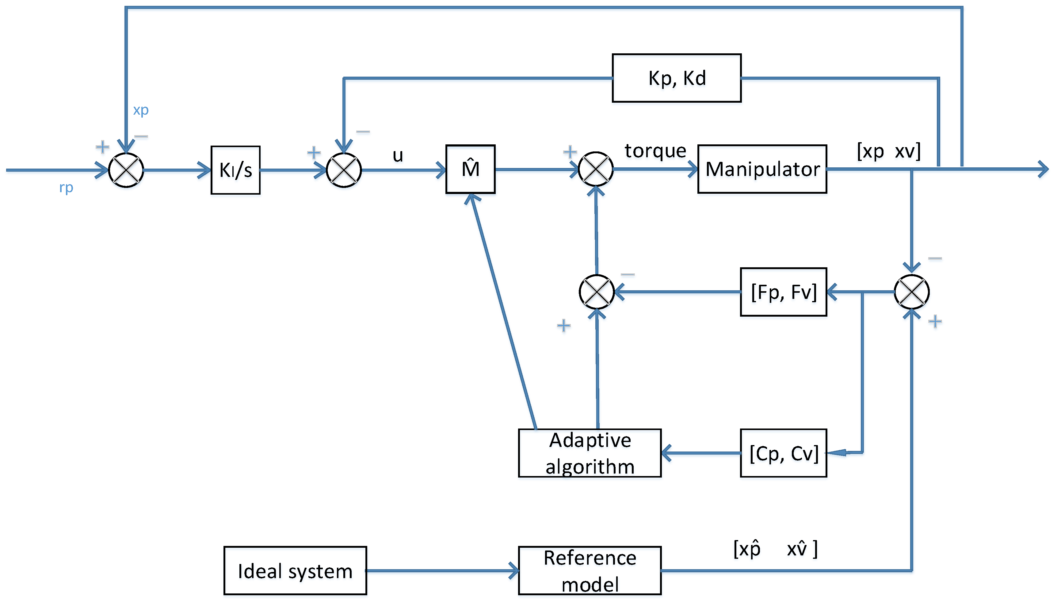Figure 4 shows a model reference control approach. The output of the reference model will be compared with the output of the manipulator (plant), which produces an error (a difference). The error will go through the adaptation mechanism to adjust the parameters of the dynamic model of the manipulator (i.e., the adaptation process section employed the difference in order to generate the input component that goes to the plant). The matrices F_p, F_v, C_p, and C_v are introduced in order to make the system stable [4]. At the same time, the plant’s output compares with the desired model, and one can therefore lead to generate another difference. This difference goes through the integration operation, and subsequently deducts the feedback position and velocity. This action resembles the PID control action. This process’ output, times the terms from the adaptation algorithm, then adding the terms from the adaptation algorithm, is the plant’s input. This operation will resume until the difference between the plant’s output and the reference model’s output equals to zero. The ideal system is cut off from the plant, meaning that the plant variables’ feedback values will not participate in handling the reference model’s input. The input to the reference model will be handled from its own output variables. The ideal system is entirely uninfluenced by the plant’s performance. As with the PID control, the output from the controller can be determined as follows. For the model reference adaptive control approach,

$$ControllerOut=\tau =\stackrel{\wedge }{M}u+\stackrel{\wedge }{V}-F_{p}e-F_v\stackrel{•}{e}$$

(10)

where $u=K_I{\displaystyle \int (r_p-x_p)}-K_p{x}_p-K_d{x}_v$.

The manipulator dynamic equation is:

$$\tau =Ma+V+Gg$$

(11)

So, the output from the manipulator (i.e., acceleration of the joint) is:

$$\stackrel{\wedge }{M}u+\stackrel{\wedge }{V}-F_{p}e-F_v\stackrel{•}{e}=\tau =Ma+V$$

$$\Rightarrow \left[\begin{array}{l}{a}_1\\ a_2\end{array}\right]=\left[\begin{array}{l}\stackrel{••}{{\theta }_1}\\ \stackrel{••}{{\theta }_2}\end{array}\right]=M^{-1}(\stackrel{\wedge }{M}u+\stackrel{\wedge }{V}-F_{p}e-F_v\stackrel{•}{e}-V)$$

(12)

After deriving the acceleration of the joint, take the time integral to obtain the velocity of the joint, and take another integral to obtain the positon of the joint. The adaptive algorithm is derived as follows. We now use the Popov’s asymptotic hyper-stability theorem [4], and set $\stackrel{\approx }{M}=\stackrel{\wedge }{M}-M$. Since:

$${\displaystyle \underset{0}{\overset{T}{\int }}{y}^T(t)}w(t)dt={\displaystyle \underset{0}{\overset{T}{\int }}{y}^T(t)}\stackrel{\approx }{M}u(t)dt+{\displaystyle \sum _{i=1}^3{\displaystyle \underset{0}{\overset{T}{\int }}{y}_i(t)}{x_v}^T}(\stackrel{\wedge }{N_i}-N_i)x_{v}dt$$

(13)

where $y=C_v\stackrel{•}{e}+C_{p}e$, and $w(t)=(\stackrel{\wedge }{M}-M)u(t)+\left[\begin{array}{l}{x_v}^T(\stackrel{\wedge }{N_1}(t)-N_1)x_v\\ {x_v}^T(\stackrel{\wedge }{N_2}(t)-N_2)x_v\\ {x_v}^T(\stackrel{\wedge }{N_3}(t)-N_3)x_v\end{array}\right]$. The first term is used to derive the adaptive algorithm for $M$, and the second term is used to derive the adaptive algorithm for $N$. For the first term:

$$\begin{array}{cc}\hfill {\displaystyle \underset{0}{\overset{T}{\int }}{y}^T(t)}\stackrel{\approx }{M}u(t)dt& ={{\displaystyle \underset{0}{\overset{T}{\int }}\left[\begin{array}{l}{y}_1\\ y_2\end{array}\right]}}^T\left[\begin{array}{cc}{\stackrel{\approx }{m}}_{11}& {\stackrel{\approx }{m}}_{12}\\ {\stackrel{\approx }{m}}_{12}& {\stackrel{\approx }{m}}_{22}\end{array}\right]\left[\begin{array}{l}{u}_1\\ u_2\end{array}\right]dt\hfill \\ & ={\displaystyle \underset{0}{\overset{T}{\int }}[y_1,y_2]}\left[\begin{array}{cc}{\stackrel{\approx }{m}}_{11}& {\stackrel{\approx }{m}}_{12}\\ {\stackrel{\approx }{m}}_{12}& {\stackrel{\approx }{m}}_{22}\end{array}\right]\left[\begin{array}{l}{u}_1\\ u_2\end{array}\right]dt\hfill \\ & ={\displaystyle \underset{0}{\overset{T}{\int }}{\stackrel{\approx }{m}}_{11}}{y}_1{u}_{1}dt+{\displaystyle \underset{0}{\overset{T}{\int }}{\stackrel{\approx }{m}}_{12}(y_1{u}_2+y_2{u}_1)dt}+{\displaystyle \underset{0}{\overset{T}{\int }}{\stackrel{\approx }{m}}_{22}}{y}_2{u}_{2}dt\hfill \end{array}$$

(14)

$\stackrel{\wedge }{M}$ and $\stackrel{\wedge }{N}$ are the adjusted parameters of the dynamic equation of the manipulator, the matrices Fp, Fv, Cp, and Cv are introduced in order to make the system stable [4], and $y(t)$ is the output from the Cp and Cv block. Consider the first term in the above equation, and based on Popov’s asymptotic hyper-stability theorem [4], to prove asymptotic convergence, it must be shown that, for all T ≥ 0, we need to find $\frac{d}{dt}\stackrel{\wedge }{m_{11}}(t)=\frac{d}{dt}\stackrel{\approx }{m_{11}}(t)$, so that ${\displaystyle \underset{0}{\overset{T}{\int }}{\stackrel{\approx }{m}}_{11}}{y}_1{u}_{1}dt\ge -{\gamma }^2$.

Where γ² is a positive constant that is a function of the initial conditions. From ${\displaystyle \underset{0}{\overset{T}{\int }}z{(t)}^T}\stackrel{•}{z(t)}dt=\frac{z{(T)}^{T}z(T)}{2}-\frac{z{(0)}^{T}z(0)}{2}\ge -\frac{z{(0)}^{T}z(0)}{2}=-{{\gamma }_0}^2$, so by selecting $\frac{d}{dt}\stackrel{\wedge }{m_{11}}(t)=\frac{d}{dt}\stackrel{\approx }{m_{11}}(t)=k_{m11}{y}_1{u}_1$, one has

$$\Rightarrow y_1{u}_1=\frac{\stackrel{•}{\stackrel{\approx }{m_{11}}(t)}}{k_{m11}}$$

(15)

Then, ${\displaystyle \underset{0}{\overset{T}{\int }}{\stackrel{\approx }{m}}_{11}}{y}_1{u}_{1}dt={\displaystyle \underset{0}{\overset{T}{\int }}{\stackrel{\approx }{m}}_{11}}\stackrel{•}{{\stackrel{\approx }{m}}_{11}}\frac{1}{k_{m11}}dt=\frac{1}{k_{m11}}{\displaystyle \underset{0}{\overset{T}{\int }}{\stackrel{\approx }{m}}_{11}}\stackrel{•}{{\stackrel{\approx }{m}}_{11}}dt\ge -{\gamma }^2$, in order to make the system stable [4].

Using the same analysis on the other two terms, we obtain

$$\frac{d}{dt}\stackrel{\wedge }{m_{12}}(t)=\frac{d}{dt}\stackrel{\approx }{m_{12}}(t)=k_{m12}(y_1{u}_2+y_2{u}_1),\frac{d}{dt}\stackrel{\wedge }{m_{22}}(t)=\frac{d}{dt}\stackrel{\approx }{m_{22}}(t)=k_{m22}{y}_2{u}_2$$

Derivation for M has finished. Now, using the same approach, we can obtain the adaptive algorithm for N as follows:

$$\frac{d}{dt}\stackrel{\wedge }{n_{12}}(t)=\frac{d}{dt}\stackrel{\approx }{n_{12}}(t)=k_{n12}(2y_1{x}_{v1}{x}_{v2}-y_2{x_{v1}}^2),\frac{d}{dt}\stackrel{\wedge }{n_{22}}(t)=\frac{d}{dt}\stackrel{\approx }{n_{22}}(t)=k_{n22}{y}_1{x_{v2}}^2$$

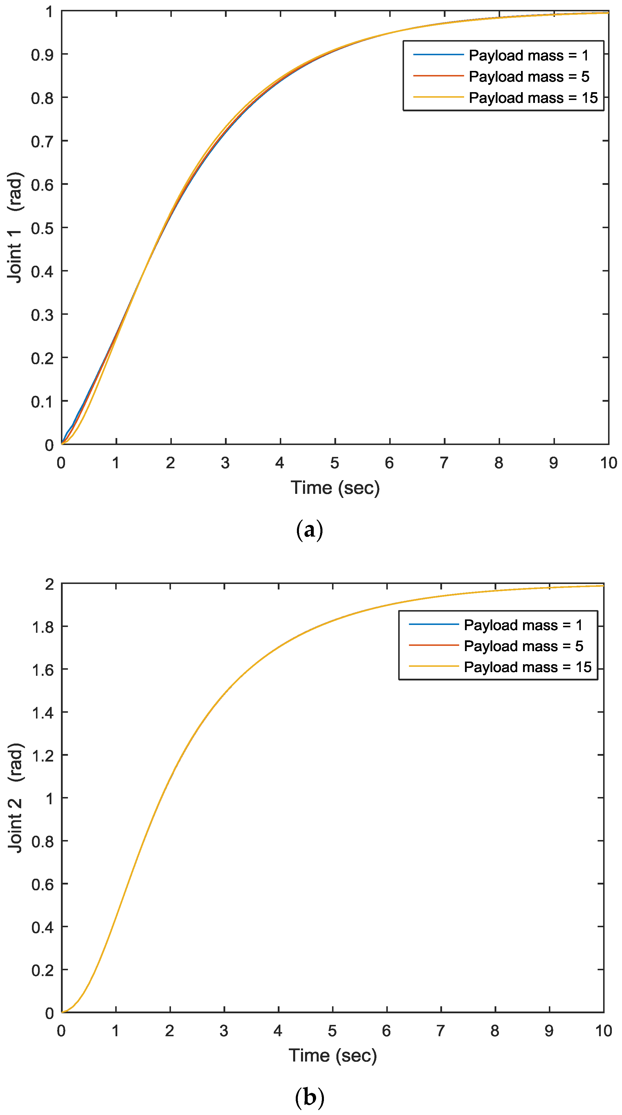
Figure 5 shows the joints’ output under different payload masses. By using the model reference adaptive control approach, three lines coincide with each other under different payload masses; i.e., the payload mass variation effect has been compensated.

2.2. Three-DOF Link Case

For the 3-DOF link case, as shown in Figure 6, by using the Lagrange method, the dynamic equation is obtained as follows. Here, we just give the results.

$$\left[\begin{array}{l}{\tau }_1\\ {\tau }_2\\ {\tau }_3\end{array}\right]=M\stackrel{••}{\theta }+N+Gg=\left[\begin{array}{ccc}{m}_{11}& m_{12}& m_{13}\\ m_{12}& m_{22}& m_{23}\\ m_{13}& m_{23}& m_{33}\end{array}\right]\left[\begin{array}{l}\stackrel{••}{{\theta }_1}\\ \stackrel{••}{{\theta }_2}\\ \stackrel{••}{{\theta }_3}\end{array}\right]+\left[\begin{array}{l}{n}_{11}\\ n_{21}\\ n_{31}\end{array}\right]+\left[\begin{array}{l}{g}_{11}\\ g_{21}\\ g_{31}\end{array}\right]g$$

(16)

where $m_{11}=m_1{a}^2+m_2{r_1}^2+m_3{r_1}^2$, $m_{12}=r_1(m_{2}b+m_3{r}_2)\cos ({\theta }_2-{\theta }_1)$, $m_{13}=m_3{r}_{1}c\cos ({\theta }_1+{\theta }_3)$ $m_{22}=m_2{b}^2+m_3{r_2}^2$, $m_{23}=m_3{r}_{2}c\cos ({\theta }_2+{\theta }_3)$, $m_{33}=m_3{c}^2$ $n_{11}=-r_1(m_{2}b+m_3{r}_2)\sin ({\theta }_2-{\theta }_1){\stackrel{•}{{\theta }_2}}^2-m_3{r}_{1}c\sin ({\theta }_1+{\theta }_3){\stackrel{•}{{\theta }_3}}^2$ $n_{21}=r_1(m_{2}b+m_3{r}_2)\sin ({\theta }_2-{\theta }_1){\stackrel{•}{{\theta }_1}}^2-m_3{r}_{2}c\sin ({\theta }_2+{\theta }_3){\stackrel{•}{{\theta }_3}}^2$ $n_{31}=-m_3{r}_{1}c\sin ({\theta }_1+{\theta }_3){\stackrel{•}{{\theta }_1}}^2-m_3{r}_{2}c\sin ({\theta }_2+{\theta }_3){\stackrel{•}{{\theta }_2}}^2$ a = l₁/2, b = l₂/2, c = l₃/2; r₁ = l₁, r₂ = l₂, r₃ = l₃.

Now apply the PID controller, the controller output is the torque,

$$K_{p}e+K_i{\displaystyle \int e}dt+K_d\stackrel{•}{e}=\left[\begin{array}{l}{\tau }_1\\ {\tau }_2\\ {\tau }_3\end{array}\right]$$

(17)

where error $e=r_p-x_p$.

Knowing the two-link manipulator M and N matrices, the output from the manipulator (i.e., acceleration of joints 1 and 2) can be determined as follows:

$$\left[\begin{array}{l}{\tau }_1\\ {\tau }_2\\ {\tau }_3\end{array}\right]=M\stackrel{••}{\theta }+N+Gg=\left[\begin{array}{ccc}{m}_{11}& m_{12}& m_{13}\\ m_{12}& m_{22}& m_{23}\\ m_{13}& m_{23}& m_{33}\end{array}\right]\left[\begin{array}{l}\stackrel{••}{{\theta }_1}\\ \stackrel{••}{{\theta }_2}\\ \stackrel{••}{{\theta }_3}\end{array}\right]+\left[\begin{array}{l}{n}_{11}\\ n_{21}\\ n_{31}\end{array}\right]+\left[\begin{array}{l}{g}_{11}\\ g_{21}\\ g_{31}\end{array}\right]g$$

(18)

So $K_{p}e+K_i{\displaystyle \int e}dt+K_d\stackrel{•}{e}=\left[\begin{array}{l}{\tau }_1\\ {\tau }_2\\ {\tau }_3\end{array}\right]=M\stackrel{••}{\theta }+N+Gg$ $\Rightarrow \left[\begin{array}{l}\stackrel{••}{{\theta }_1}\\ \stackrel{••}{{\theta }_2}\end{array}\right]=M^{-1}(K_{p}e+K_i{\displaystyle \int e}dt+K_d\stackrel{•}{e}-N)$.

After deriving the acceleration of joints 1 and 2, take the time integral to obtain the velocity of joints 1 and 2, and take another integral to obtain the positon of joints 1 and 2.

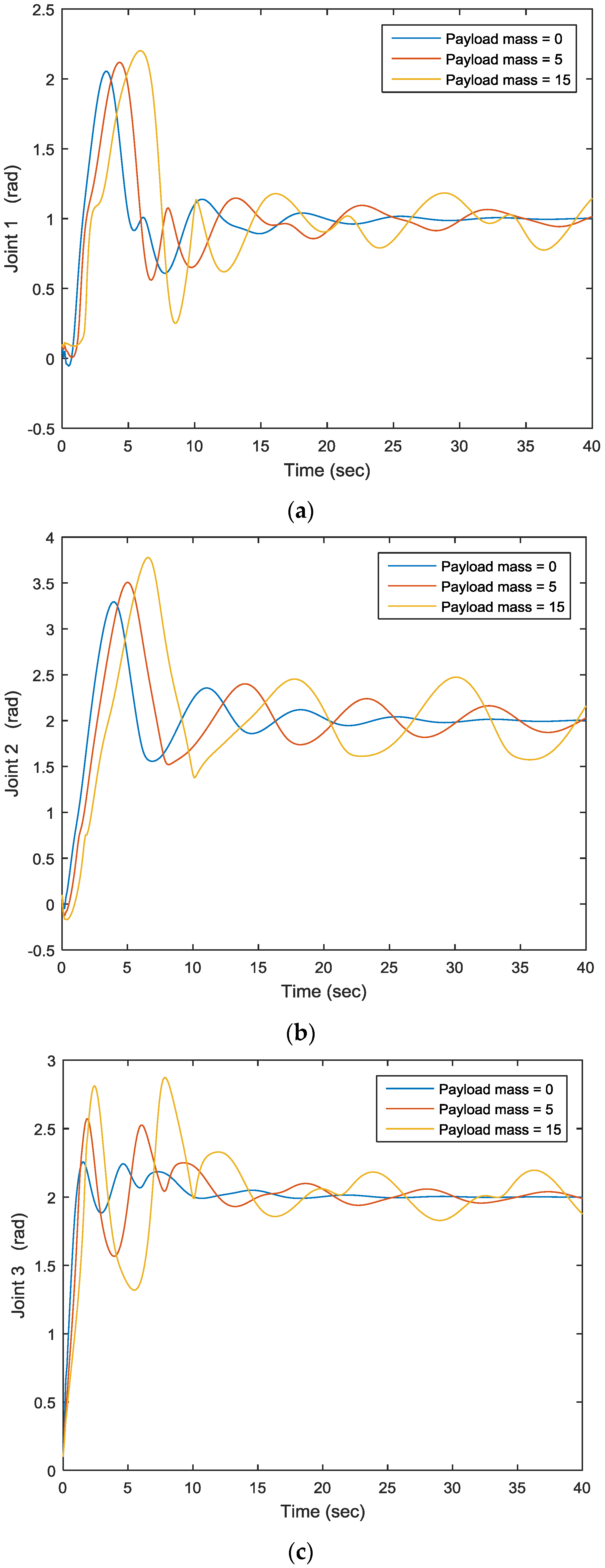
After applying different payload masses, the joints’ motion outputs are illustrated in Figure 7. For joint 1, when the payload is 0, joint one’s motion is quite steady; however, when the payload increases to 5 and 15, one can see that joint 1’s motion is not the same anymore. The same applies to joints 2 and 3. For the model reference adaptive control approach,

$$ControllerOut=\tau =\stackrel{\wedge }{M}u+\stackrel{\wedge }{V}-F_{p}e-F_v\stackrel{•}{e}$$

(19)

where $u=K_I{\displaystyle \int (r_p-x_p)}-K_p{x}_p-K_d{x}_v$.

So, the output from the manipulator (i.e., acceleration of joint) is:

$$\stackrel{\wedge }{M}u+\stackrel{\wedge }{V}-F_{p}e-F_v\stackrel{•}{e}=\tau =Ma+V\Rightarrow \left[\begin{array}{l}{a}_1\\ a_2\\ a_3\end{array}\right]=\left[\begin{array}{l}\stackrel{••}{{\theta }_1}\\ \stackrel{••}{{\theta }_2}\\ \stackrel{••}{{\theta }_3}\end{array}\right]=M^{-1}(\stackrel{\wedge }{M}u+\stackrel{\wedge }{V}-F_{p}e-F_v\stackrel{•}{e}-V)$$

(20)

After deriving the acceleration of the joint, take the time integral to obtain the velocity of the joint and take another integral to obtain the positon of the joint. By using the same approach, the adaptive algorithm is derived as follows:

$$\begin{array}{l}\frac{d}{dt}\stackrel{\wedge }{m_{11}}(t)=\frac{d}{dt}\stackrel{\approx }{m_{11}}(t)=k_{m11}{y}_1{u}_1,\frac{d}{dt}\stackrel{\wedge }{m_{12}}(t)=\frac{d}{dt}\stackrel{\approx }{m_{12}}(t)=k_{m12}(y_1{u}_2+y_2{u}_1)\\ \frac{d}{dt}\stackrel{\wedge }{m_{13}}(t)=\frac{d}{dt}\stackrel{\approx }{m_{13}}(t)=k_{m13}(y_3{u}_1+y_1{u}_3),\frac{d}{dt}\stackrel{\wedge }{m_{22}}(t)=\frac{d}{dt}\stackrel{\approx }{m_{22}}(t)=k_{m22}{y}_2{u}_2\\ \frac{d}{dt}\stackrel{\wedge }{m_{23}}(t)=\frac{d}{dt}\stackrel{\approx }{m_{23}}(t)=k_{m23}(y_3{u}_2+y_2{u}_3),\frac{d}{dt}\stackrel{\wedge }{m_{33}}(t)=\frac{d}{dt}\stackrel{\approx }{m_{33}}(t)=k_{m33}{y}_3{u}_3\\ \frac{d}{dt}\stackrel{\wedge }{n_{12}}(t)=\frac{d}{dt}\stackrel{\approx }{n_{12}}(t)=k_{n12}(2y_1{x}_{v1}{x}_{v2}-y_2{x_{v1}}^2),\frac{d}{dt}\stackrel{\wedge }{n_{13}}(t)=\frac{d}{dt}\stackrel{\approx }{n_{13}}(t)=k_{n13}(2y_1{x}_{v1}{x}_{v3}-y_3{x_{v1}}^2)\\ \frac{d}{dt}\stackrel{\wedge }{n_{22}}(t)=\frac{d}{dt}\stackrel{\approx }{n_{22}}(t)=k_{n22}{y}_1{x_{v2}}^2,\frac{d}{dt}\stackrel{\wedge }{{n_{33}}^1}(t)=\frac{d}{dt}\stackrel{\approx }{{n_{13}}^1}(t)=k_{n33}^1(2y_1{x}_{v2}{x}_{v3}-y_1{x_{v3}}^2)\\ \frac{d}{dt}\stackrel{\wedge }{{n_{33}}^2}(t)=\frac{d}{dt}\stackrel{\approx }{{n_{13}}^2}(t)=k_{n33}^2(2y_2{x}_{v2}{x}_{v3}+y_2{x_{v3}}^2-y_3{x_{v2}}^2).\end{array}$$

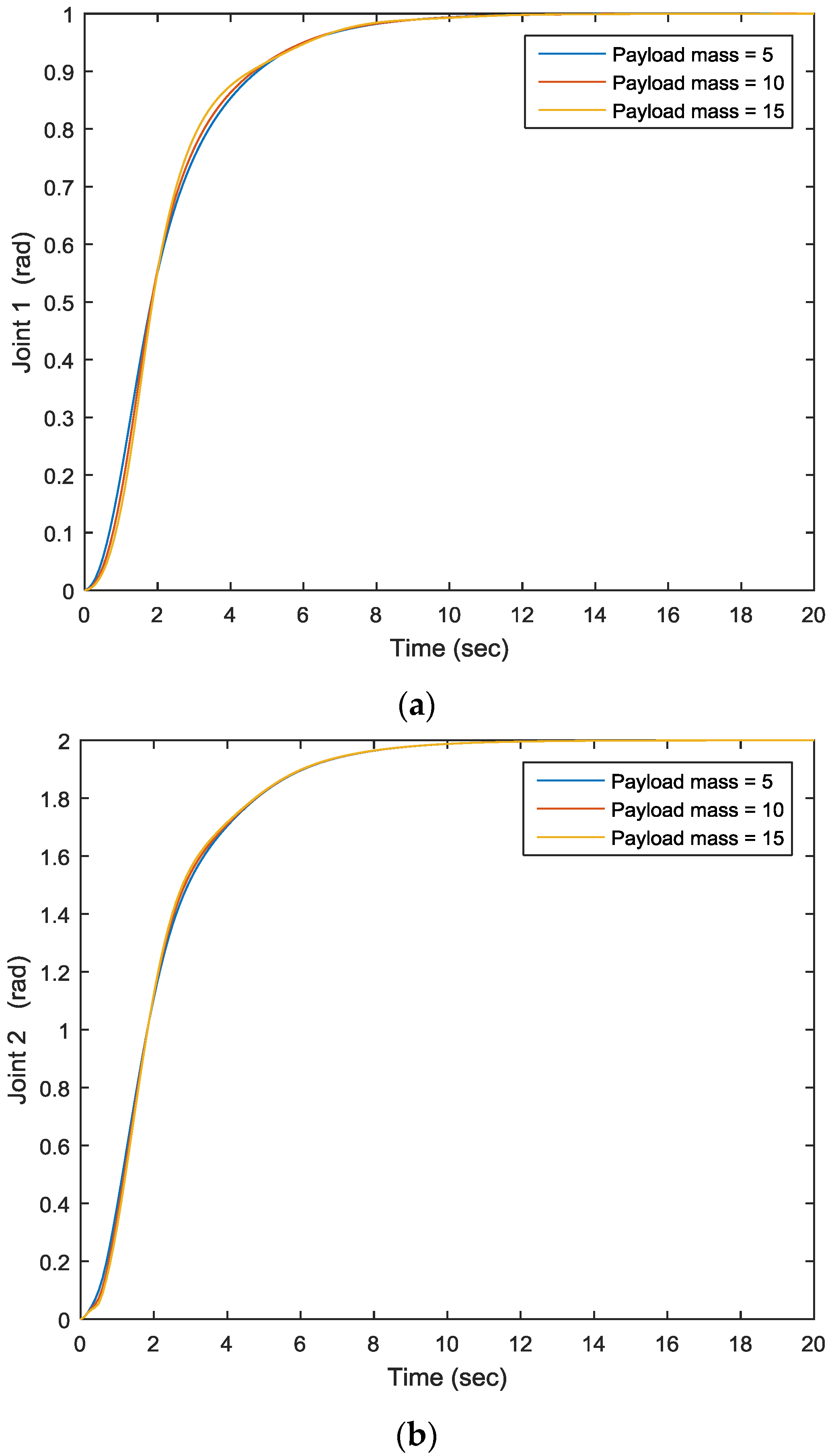
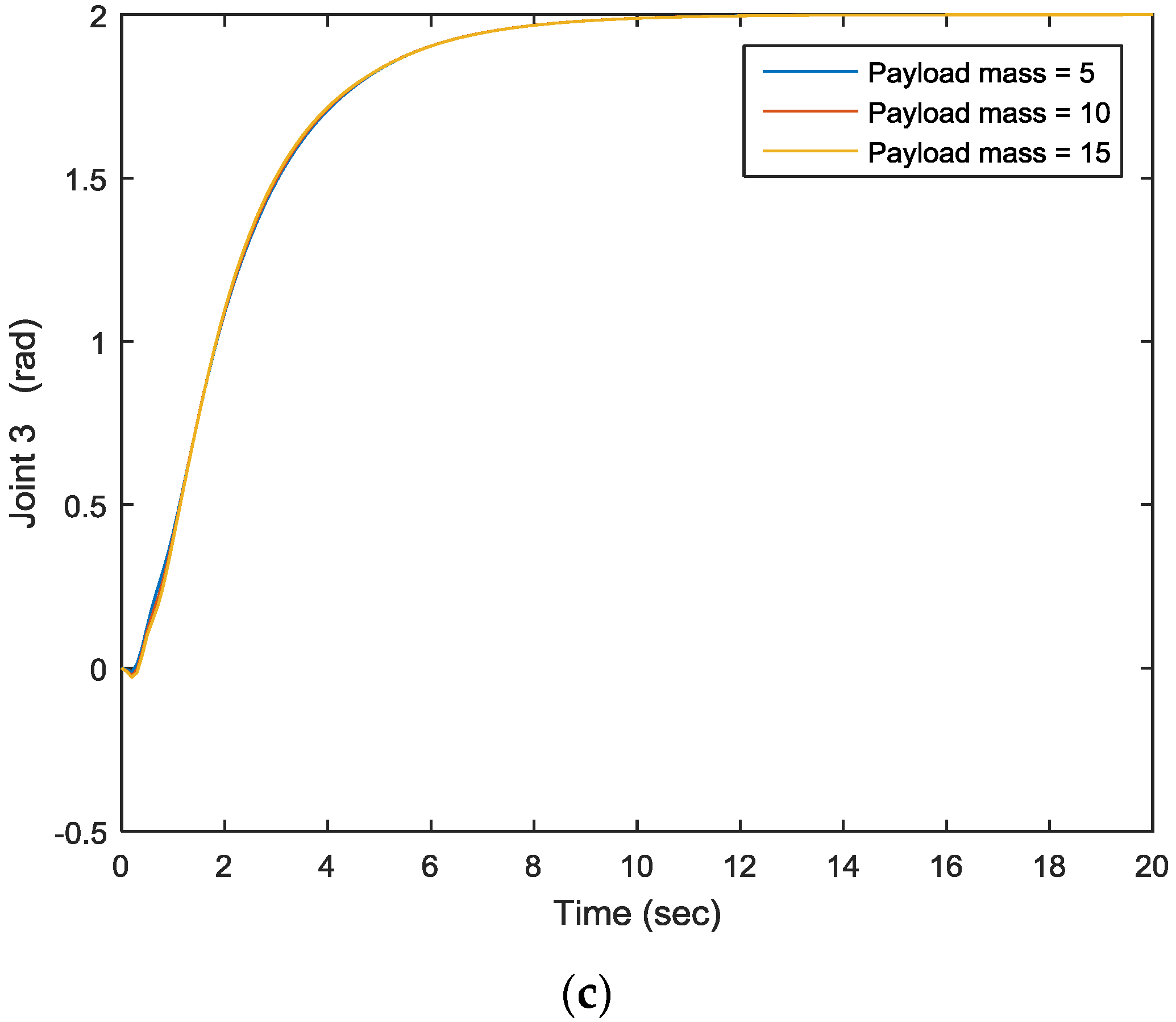
Figure 8 shows the joints’ output under different payload masses. By using the model reference adaptive control approach, the variation effect of payload mass has been resolved. One can see that three lines coincide with each other under different payload masses; i.e., the payload mass variation effect has been compensated.

3. Conclusions

When the end-effector grasps different payload masses, the output of joint motion will vary, which will decrease the positioning accuracy of the end-effector. Based on the model reference adaptive control approach, the payload variation effect can be solved effectively, therefore improving the positioning accuracy. Comparing the simulated results with the behavior of a real kinematic and experimental evaluation will be our future work. In addition, future research will focus on hybrid control design by combining model reference adaptive control and PID control for serial robotic arms.