A Novel Design for Adjustable Stiffness Artificial Tendon for the Ankle Joint of a Bipedal Robot: Modeling & Simulation

Abstract

Bipedal humanoid robots are expected to play a major role in the future. Performing bipedal locomotion requires high energy due to the high torque that needs to be provided by its legs’ joints. Taking the WABIAN-2R as an example, it uses harmonic gears in its joint to increase the torque. However, using such a mechanism increases the weight of the legs and therefore increases energy consumption. Therefore, the idea of developing a mechanism with adjustable stiffness to be connected to the leg joint is introduced here. The proposed mechanism would have the ability to provide passive and active motion. The mechanism would be attached to the ankle pitch joint as an artificial tendon. Using computer simulations, the dynamical performance of the mechanism is analytically evaluated.

1. Introduction

Humanoid robots are expecting to play a major role in the future for performing tasks such as medical care, housework, entertainment, search and rescue, and many other tasks. The robot locomotion is an important point in developing a highly effective robot system. Recently, there have been some robots developed to perform indoor tasks such as cleaning and monitoring. Those robots use wheeled locomotion to move inside the human working environment. However, wheeled locomotion has some limitations, such as climbing the stairs and overcoming obstacles. The use of legged locomotion can overcome the limitations of wheeled locomotion. Moreover, legs are important to make the robot look more human, which would make the robot more adaptable within a human environment [1,2].

Many research achievements have been made to develop humanoid robots capable of coexisting with humans and performing a variety of tasks. For example, a research group in HONDA has developed the humanoid robots—P2, P3, and ASIMO [3]. The Japanese National Institute of Advanced Industrial Science and Technology (AIST) and Kawada Industries, Inc. have developed HRP-2P, HRP-3, and HRP-4 [2]. The Korea Advanced Institute of Science and Technology (KAIST) also developed a 40-DOF humanoid robot HUBO-2 that is capable of walking and running [4]. Waseda University has a long history of developing humanoid robots, from the WABOT-1 in 1973, which was the first humanoid robot in history, to the WABIAN-2R, which is capable of various walking motions similar to human walking [5,6].

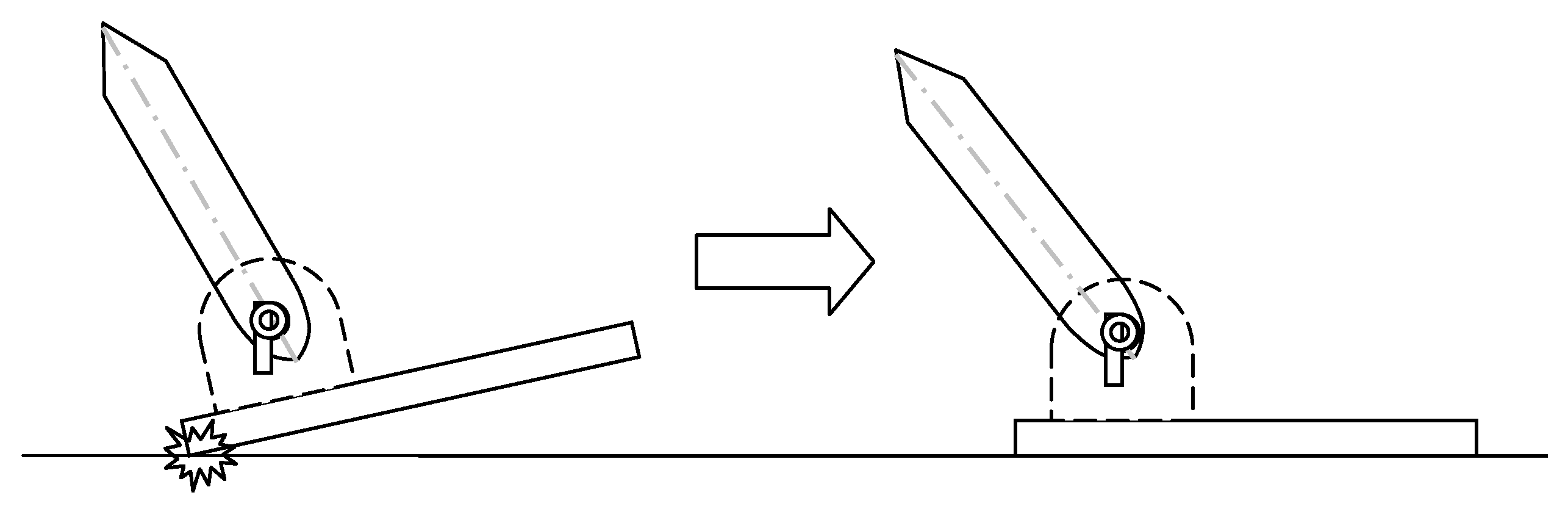
The vast majority of bipedal robots use precise joint position control for locomotion performance. This is called active walking, for which all robot’s actuators are fully powered. Those fully powered robots can do various tasks with reasonable speed and position accuracy at the cost of high control efforts, low energy efficiencies, and, most of the time, unnatural gaits. On the other hand, there are other types of robots that can perform passive walking. They are mainly referred to as passive-dynamic walking robots. These robots have been developed by researchers to mimic human walking. The main goal of building passive-dynamic walking robots is to study the role of natural dynamics in bipedal walking. Passive-dynamic walkers use gravitational energy to walk down a ramp without any actuators [7,8,9,10,11]. They are highly energy efficient but have weak stability in terms of controlling the walking motion.

Recently, to overcome the limitations and disadvantages of both active and passive walking robots, researchers have proposed a hybrid type of walking technique that could include the advantages of both walking types. Researchers are trying to reach a hybrid walking type using two approaches. The first approach is from the active side, which is done by adapting passive dynamic behavior to reduce the amount of torque driven by the actuator. The natural dynamic behavior could be achieved by controlling the joints’ torque and angle trajectory, as in the case of CB and eMOSAIC developed by ATR [12,13]. Another method for adapting natural dynamic behavior is by using actuators with compliant behavior, as in the case of Lucy [14,15]. The second approach is from the passive walking side. In this approach, direct drive or elastic actuators are installed in some of the joints of the passive-dynamic walker. Examples for successful dynamic walking robots with this approach are the Cornell Robot, Denise and Toddler [5,16]. The development of an optimal design of a bipedal robot system that has high stability locomotion with high-energy efficiency has not been achieved.

Inspired by human and animal locomotion, researchers are trying to develop a highly efficient legged locomotion system. Studies conducted on animal locomotion have discovered the effect of the muscle system as the source of driving motion. In addition to the ability of the muscle to provide motion, it has the ability to produce elastic motion [17]. The muscle’s activity could be modeled as a combination of two mechanisms connected in parallel; one mechanism is active, and the other is passive. The active mechanism is acting as an actuator, and the passive mechanism is acting similar to a nonlinear spring [18,19]. The human’s muscle plays a major role in controlling the locomotion with high-energy efficiency [20,21].

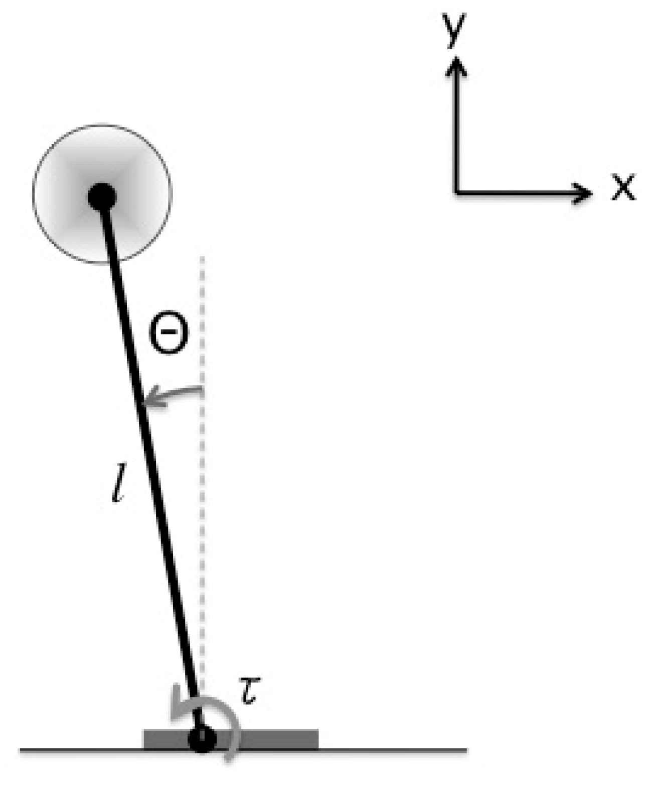
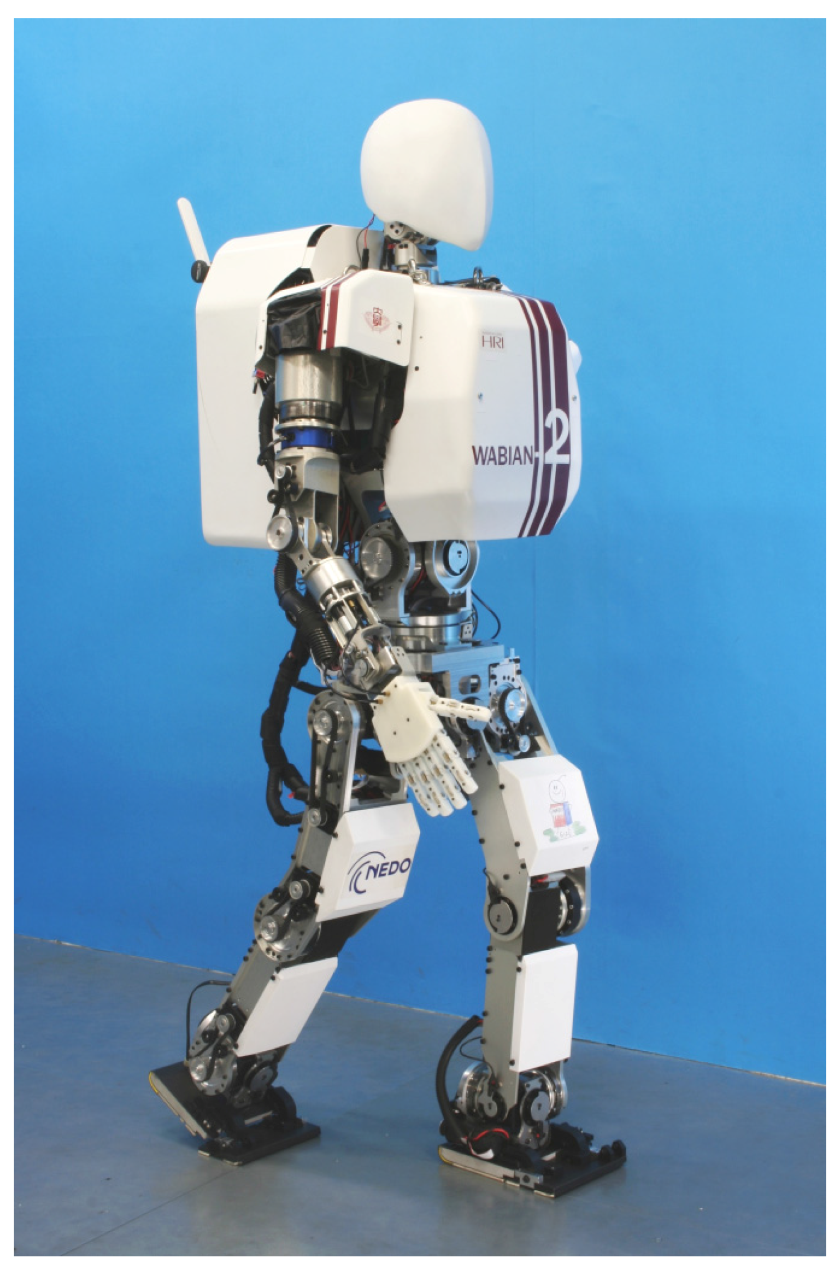
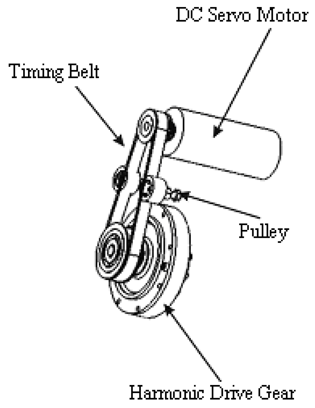
The bipedal humanoid robot WABIAN-2R (Figure 1) was developed in the Takanishi laboratory to be used as a human motion simulator [6]. The WABIAN-2R uses a harmonic drive gear (Figure 2) with a high ratio in order to provide high torque to the leg’s joints for stable walking motion. Such a harmonic drive gear requires high-energy consumption from the motor due to the mechanism's large size, which would probably have high energy loss during motion. We proposed the idea of implementing the passive dynamic walking technique into the WABIAN-2R’s walking motion [22]. Using computer simulations, we were able to simulate semi-passive dynamic walking by adding a controllable stiffness mechanism to the ankle pitch joint of the right leg [23] and by switching between active and passive rotational motion in the ankle pitch joint in both legs [24]. We tried to develop an adjustable stiffness mechanism to be added to the robot’s ankle joint in order to realize the semi-passive dynamic walking technique [25].

Figure 1. The WABIAN-2R.

Figure 1. The WABIAN-2R.

Figure 2. Joint gear system.

Figure 2. Joint gear system.

In order to implement the semi-passive dynamic walking technique into the WABIAN-2R, we need to have a mechanism that is capable of switching between active and passive motion. There were some attempts to develop such a mechanism for a bipedal walking robot in [26], which was a lightweight bipedal robot. However, the development of a mechanism that can provide hybrid motion for a full size humanoid robot has not been done. In this paper, we propose a design for a bi-directional adjustable stiffness mechanism that can be attached to the ankle joint of the WABIAN-2R. The proposed design can provide the capability of switching between active and passive rotational motion. Moreover, the mechanism could provide controllability of the stiffness of the ankle joint. Using computer simulations, we tested the performance of the mechanism and checked its ability to provide passive and active rotational motion. The simulation data tells us the effectiveness of such a mechanism design and the challenges of developing a real hardware prototype.

2. Analysis of the Ankle Joint’s Motion Performance

The ankle joint in the WABIAN-2R is made up of a DC Servomotor, a Harmonic Gear, and a Timing Belt that connect them (Figure 2). In order to reduce the energy used during walking motion, we have proposed replacing the Harmonic drive gear system with a rotational spring mechanism. Using computer simulations, we tested the performance of the ankle joint (this technique was implemented using the right leg only) [22,23,24]. 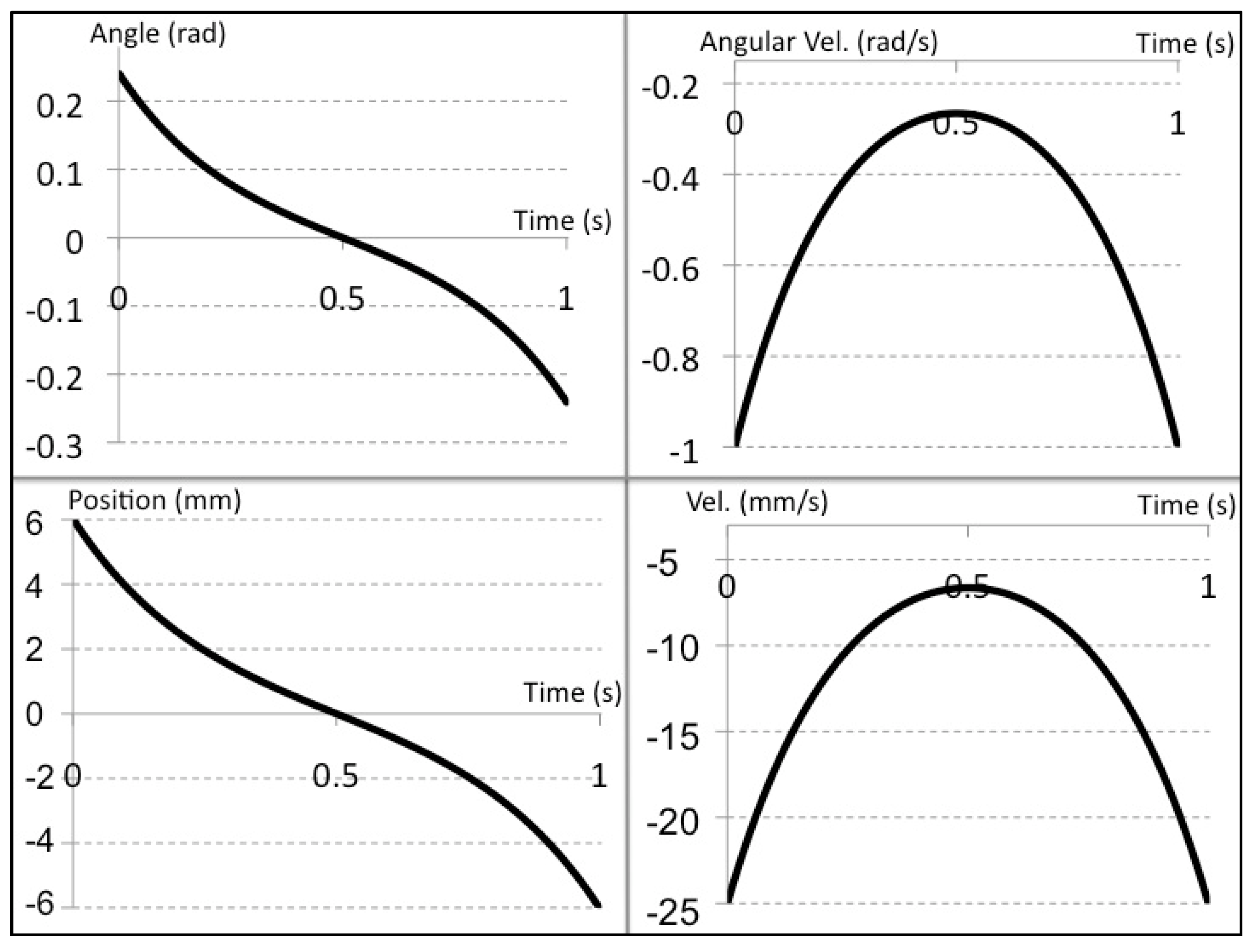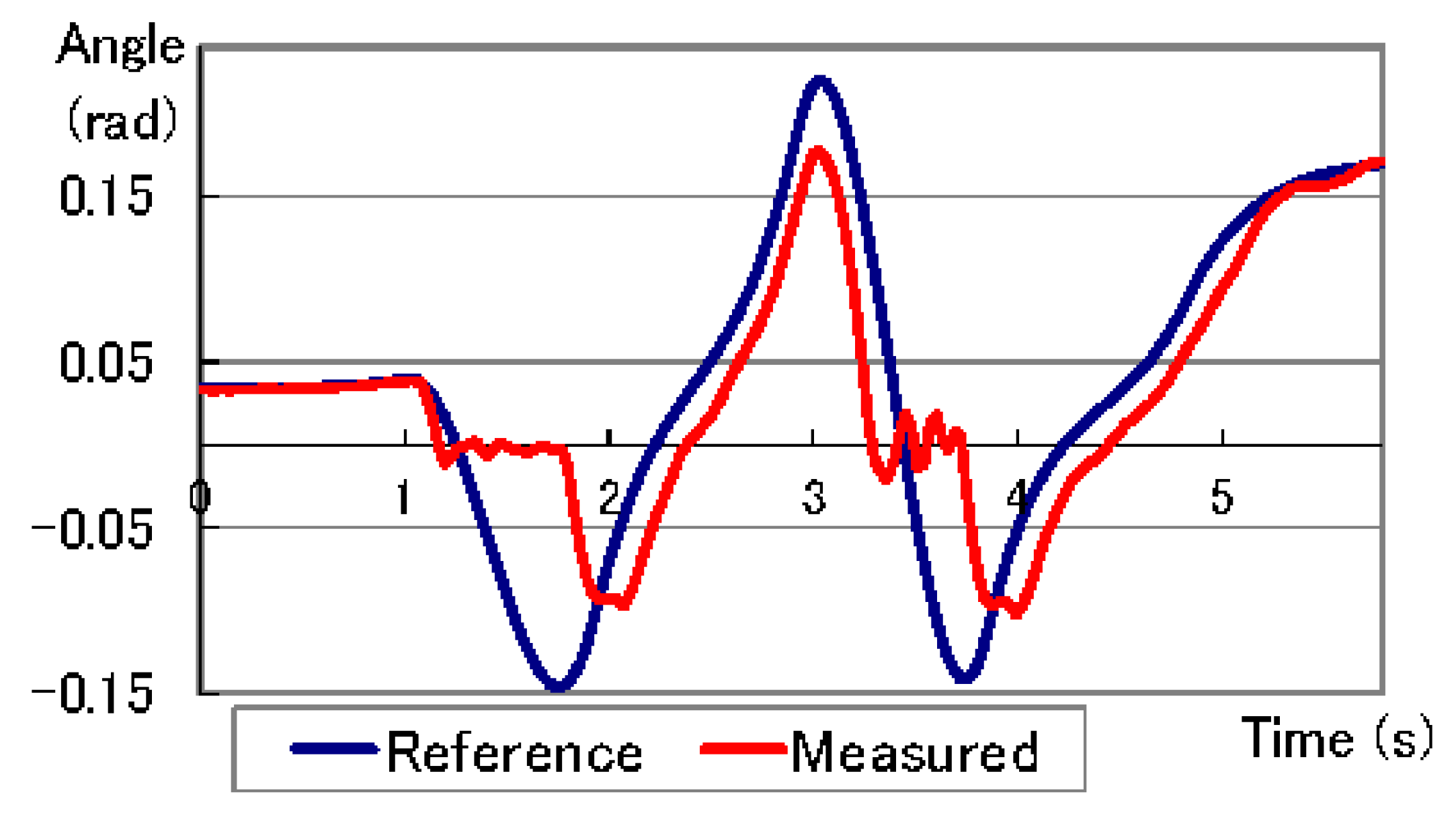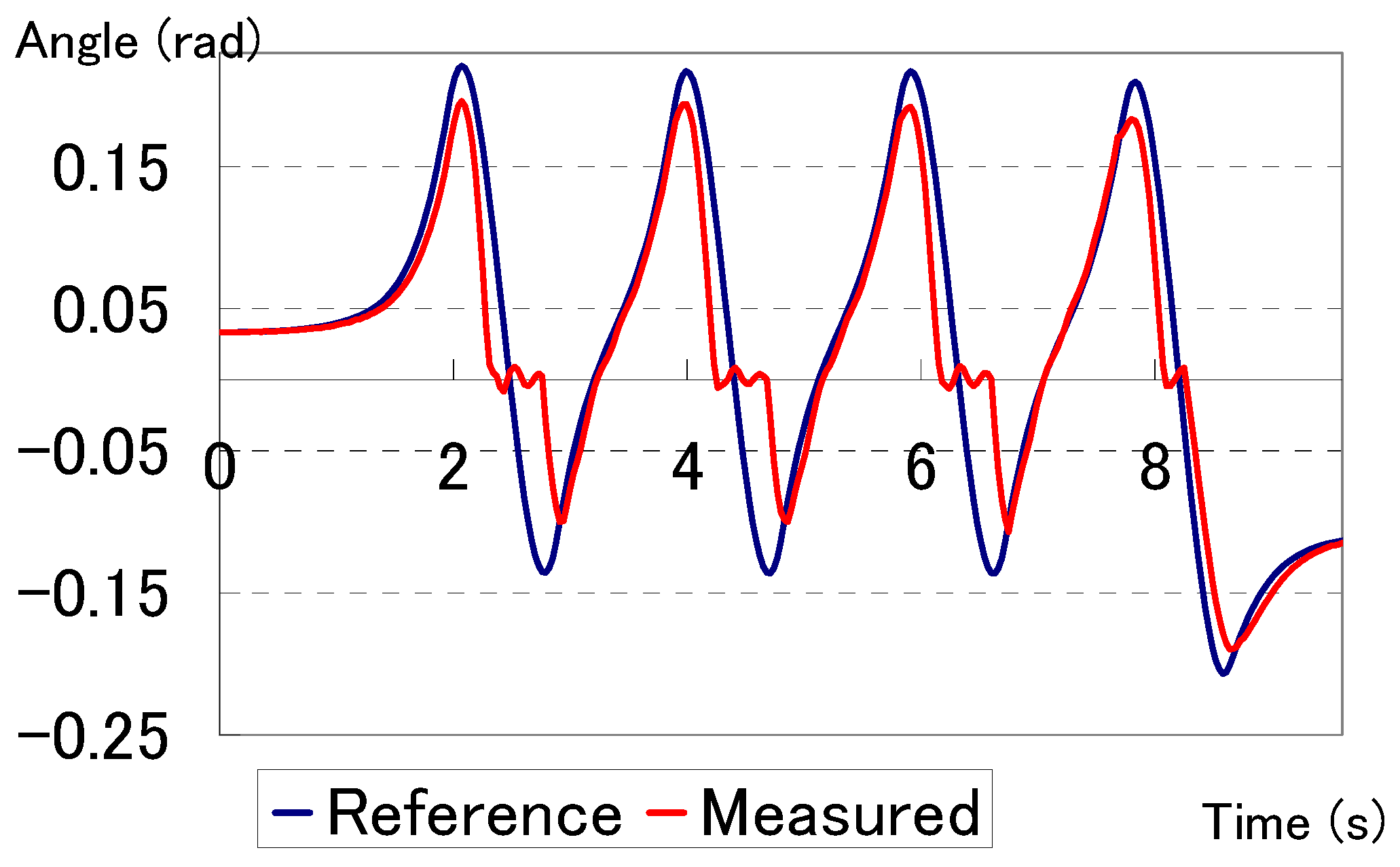Figure 3 shows both the passive motion of the ankle joint position (red line) and the reference position for the walking trajectory in active motion (blue line). 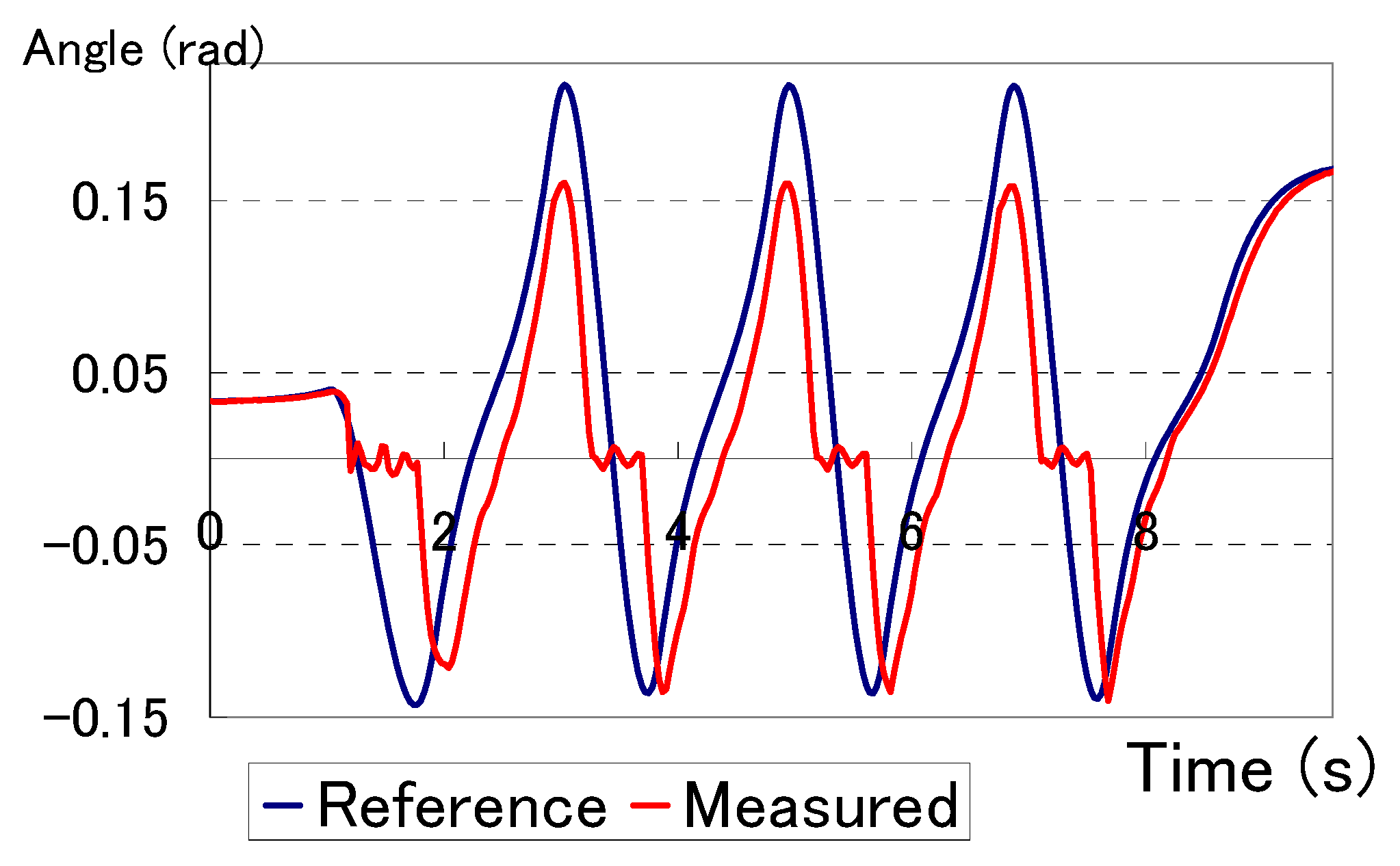Figure 4 and Figure 5 show the ankle joint position in both legs [25], which has a hybrid control that switches between passive and active mode. Using the data we got from the simulation, we were able to determine the parameter values for the developed mechanism. The data show a range of motion within ±0.23 rad; we will use this motion range as our reference when evaluating the ankle joint with the new design.

Figure 3. Position of the right ankle pitch joint for one leg passive walking.

Figure 3. Position of the right ankle pitch joint for one leg passive walking.

Figure 4. Position of the right ankle pitch joint for hybrid walking control.

Figure 4. Position of the right ankle pitch joint for hybrid walking control.

Figure 5. Position of the left ankle pitch joint for hybrid walking control.

Figure 5. Position of the left ankle pitch joint for hybrid walking control.

3. Design of the Bi-Directional Adjustable Stiffness Artificial Tendon

The main characteristic of a leg’s joint is that it should provide enough torque to support the locomotion. Designing an actuated joint that can provide high torque while keeping low energy consumption is a great challenge. One of the most successful research achievements in designing such a joint is the design made in [27]. The actuator design of [27] can provide high torque and low energy consumption for the knee joint of a prosthetic leg. Inspired by the design presented in [27], we proposed a novel design for providing rotational motion for the ankle pitch joint of the WABIAN-2R.

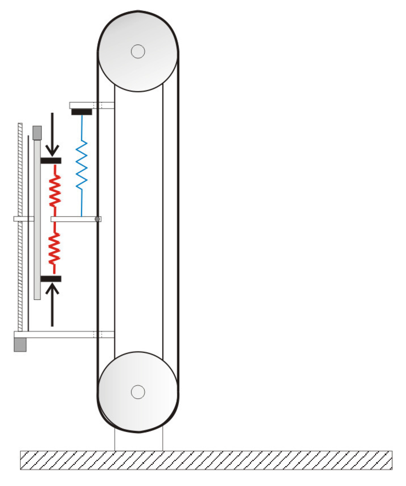
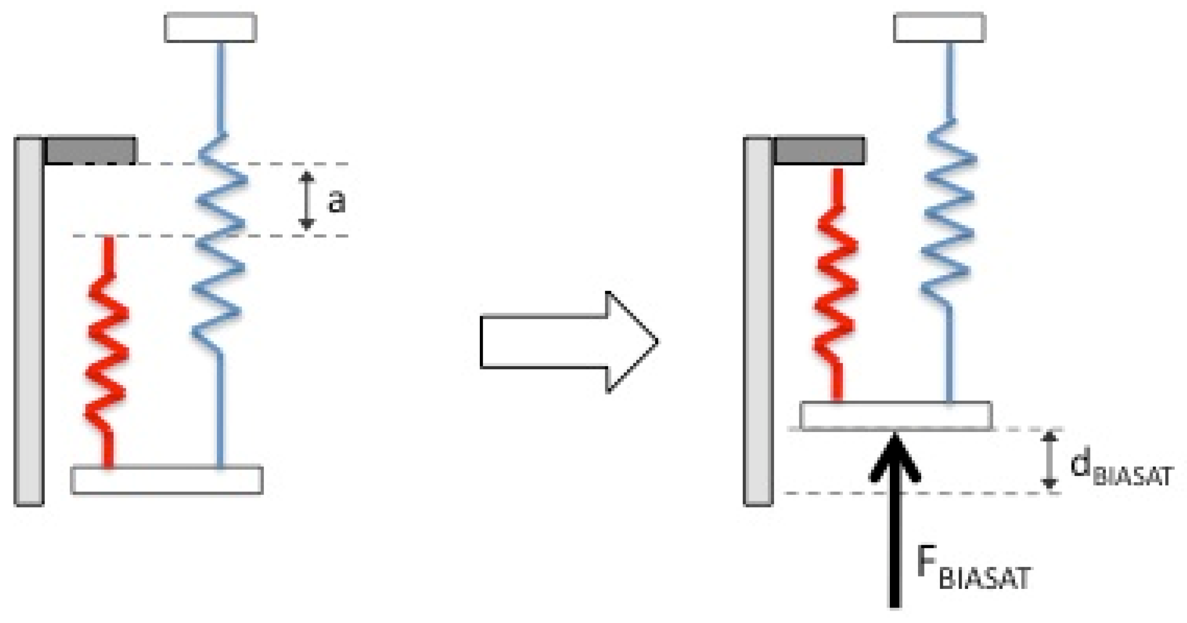
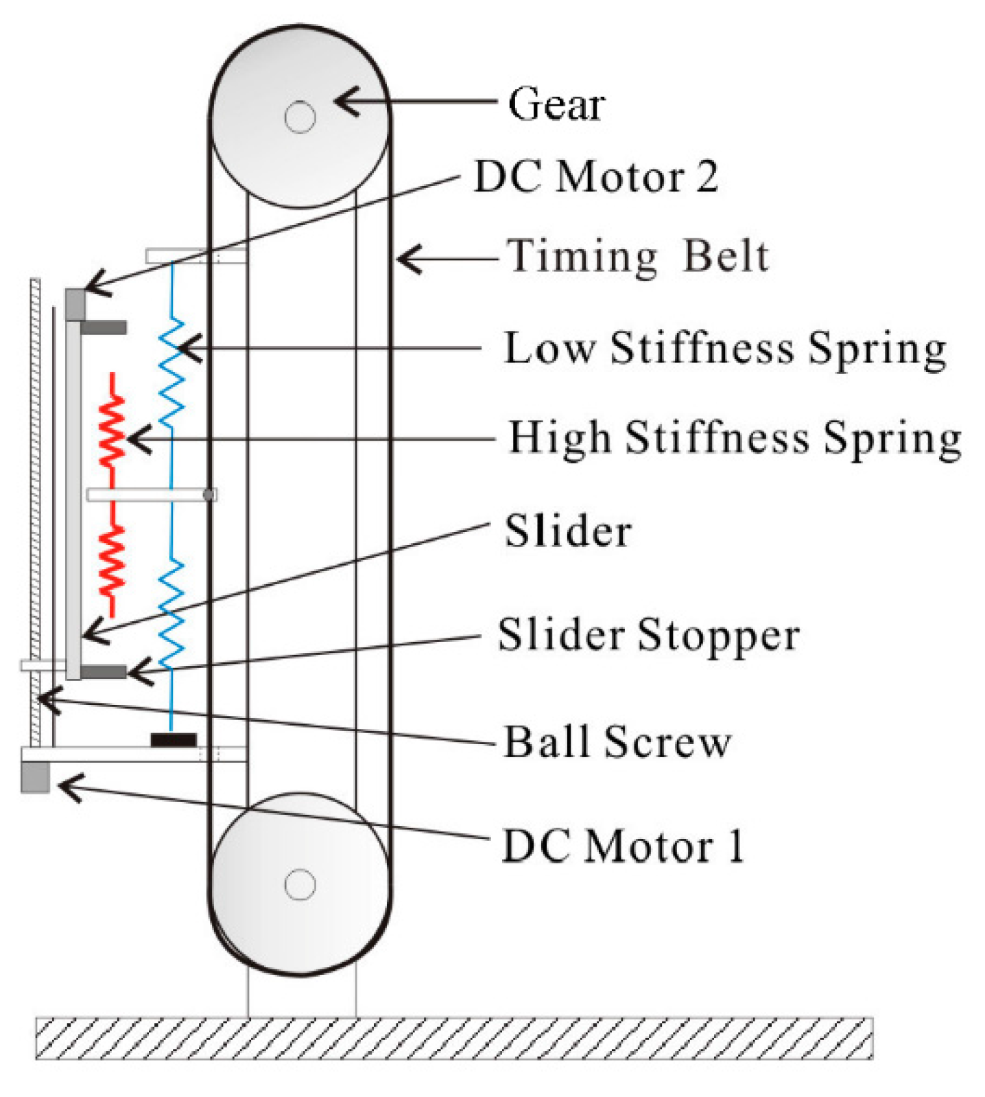
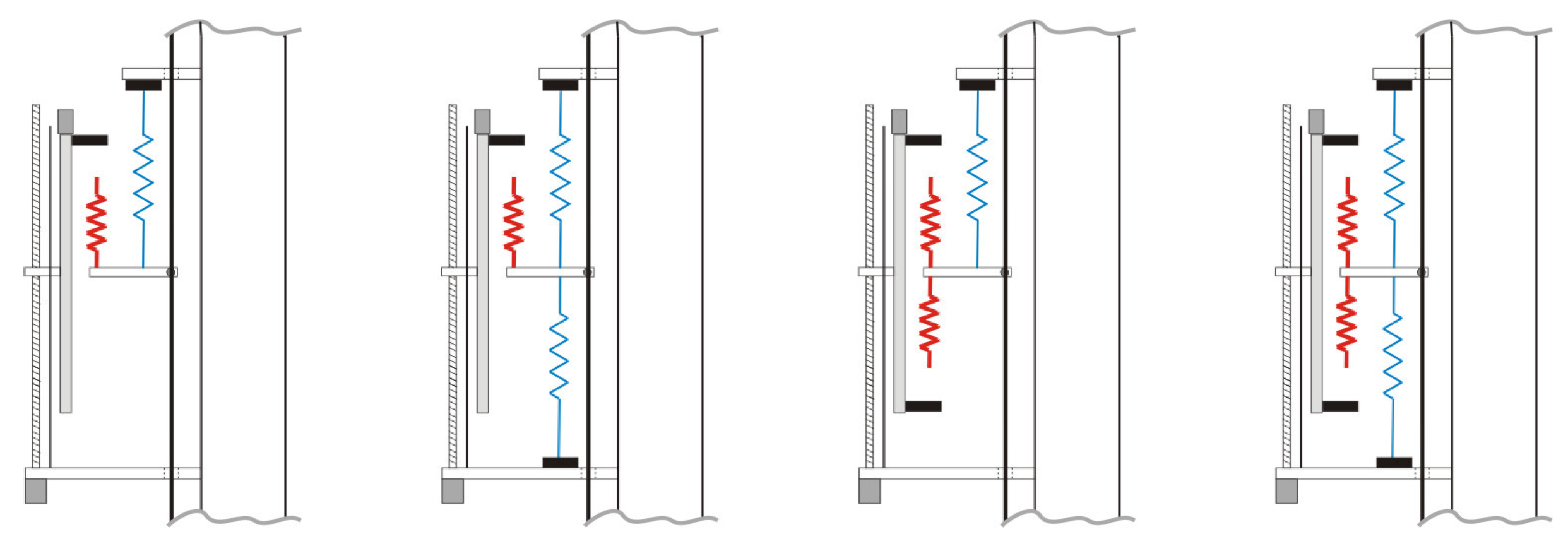
Our proposed design is an adjustable stiffness mechanism that would be able to provide the ankle joint with a hybrid type of rotational motion. The redesigned ankle joint would have the capability of switching between passive and active motion. We called the proposed mechanism a “Bi-directional Adjustable Stiffness Artificial Tendon” (BIASAT). 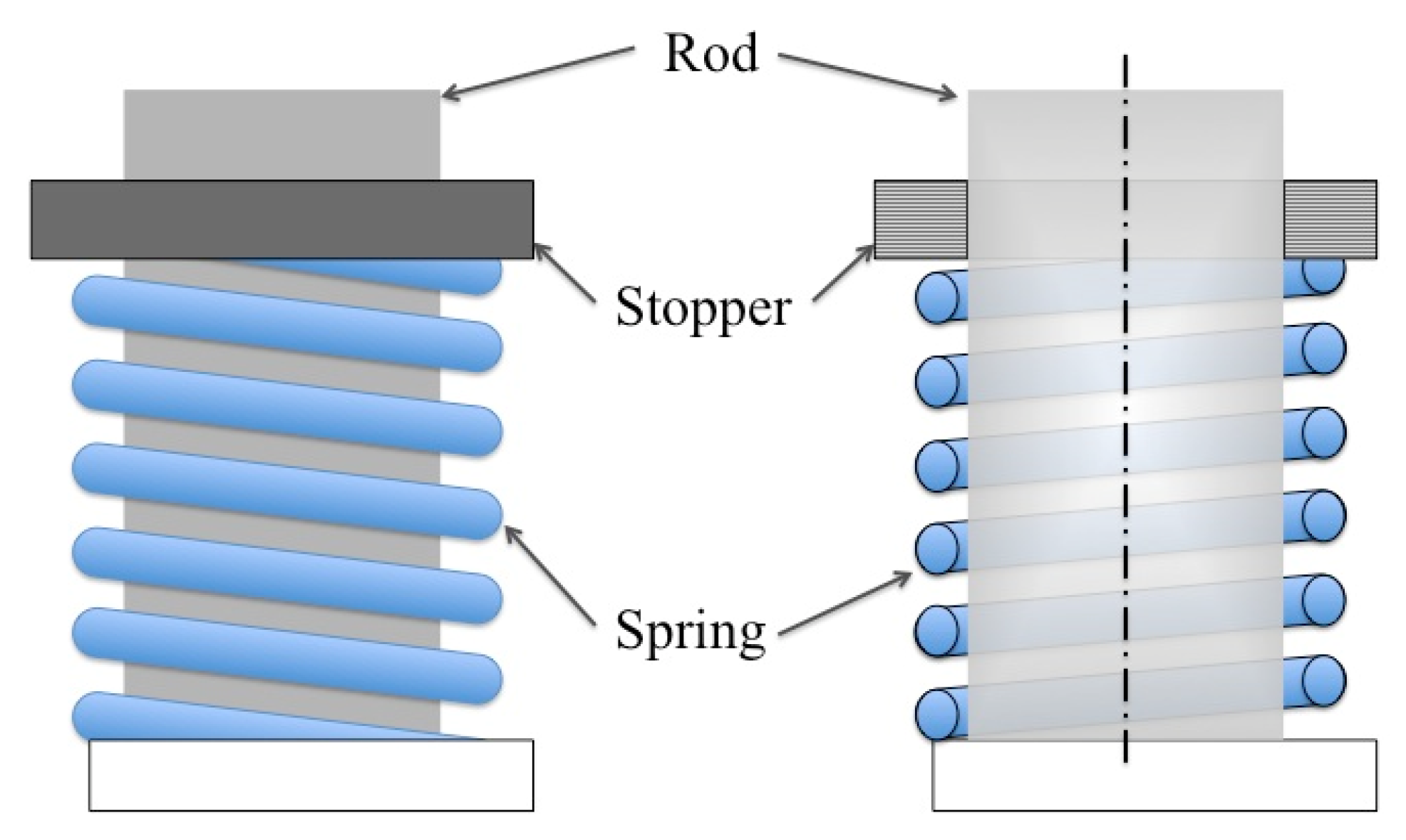As shown in Figure 6, the mechanism consists of two sets of parallel compression springs with different stiffness values and with an offset (Figure 7) connected to the output link. The output link is connected to a timing belt, which goes around the gear directly attached to the ankle pitch joint. A rod is placed inside each spring to keep it upright and to prevent it from bending or slipping (Figure 8). The two springs have an offset between them with a constant value (Figure 7). The input link is connected to Spring 1 (with low stiffness). The input link is also connected to a moveable slider mechanism with a ball screw rotated by an actuator (DC Motor 1) that positions the slider (Figure 6). The slider mechanism differentially adapts the offset between Spring 1 (low stiffness) and Spring 2 (high stiffness). Thus, it increases the stiffness in one direction and at the same time decreases in the other direction. On the other hand, the second actuator (DC Motor 2) can be used to control the position of both stoppers, which can increase or decrease the offset in both direction. Unlike the first actuator, the second actuator can be used to increase the stiffness in both directions. DC Motor 2 has an advantage in the controllability of the tendon stiffness that can control switching between active and passive modes.

Figure 6. Design outline of the BIASAT mechanism attached to the ankle pitch joint.

Figure 6. Design outline of the BIASAT mechanism attached to the ankle pitch joint.

Figure 7. Schematic of the BIASAT mechanism.

Figure 7. Schematic of the BIASAT mechanism.

Figure 8. The model of spring mechanism with the rod.

Figure 8. The model of spring mechanism with the rod.

The distance a, which is the distance between the high stiffness spring endpoint and the slider stopper, is a controllable parameter (Figure 7). The closer the stopper is to the spring, the greater the potential output of the applied force. The applied force, F_BIASAT, could be determined as follows:

$${\mathrm{F}}_{\mathrm{BIASAT}}=\{\begin{array}{cc}{\mathrm{K} }_{\mathrm{s}\mathrm{p}1}{\mathrm{d}}_{\mathrm{BIASAT}}& {\mathrm{d}}_{\mathrm{BIASAT}}<\mathrm{a}\\ {\mathrm{K} }_{\mathrm{s}\mathrm{p}1}\mathrm{a}+\left({\mathrm{K} }_{\mathrm{s}\mathrm{p}1}+{\mathrm{K} }_{\mathrm{s}\mathrm{p}2}\right)\left({\mathrm{d}}_{\mathrm{BIASAT}}-\mathrm{a}\right)& {\mathrm{d}}_{\mathrm{BIASAT}}\ge \mathrm{a}\end{array}$$

(1)

where K_sp1 is the stiffness of Spring 1 (low stiffness), K_sp2 is the stiffness of Spring 2 (high stiffness), a is the offset (distance between the spring endpoint and the stopper), and d_BIASAT is the spring’s deflection at the end point. Equation (1) could be reformed to a dimensionless form in which K_SP2 is replaced by ηK_sp1, which is as follows:

$$\frac{{\mathrm{F}}_{\mathrm{BIASAT}}}{{\mathrm{K} }_{\mathrm{s}\mathrm{p}1}\mathrm{a}}=\{\begin{array}{cc}\frac{{\mathrm{d}}_{\mathrm{BIASAT}}}{\mathrm{a}}& \frac{{\mathrm{d}}_{\mathrm{BIASAT}}}{\mathrm{a}}<1\\ 1+\left(1+\mathsf{\eta }\right)\left(\frac{{\mathrm{d}}_{\mathrm{BIASAT}}}{\mathrm{a}}-1\right)& \frac{{\mathrm{d}}_{\mathrm{BIASAT}}}{\mathrm{a}}\ge 1\end{array}$$

(2)

The force-deflection graph of the BIASAT is illustrated in Figure 8. η is the ratio of the stiffness of Spring 2 to that of Spring 1 (η = [0, 2, 5] in Figure 9). The slopes of the straight lines in Figure 8 represent the stiffness of the BIASAT. The stiffness is suddenly switched from the stiffness of Spring 1, K_sp1, to the stiffness of two parallel springs, (η + 1) K_sp1, at point d_BIASAT = a.

Figure 9. Dimensionless force-deformation graph of BIASAT in passive mode for different η values.

Figure 9. Dimensionless force-deformation graph of BIASAT in passive mode for different η values.

The mechanical design of the BIASAT has the advantage of switching between passive and active modes. Pushing into the two high stiffness springs using DC Motor 2, as shown in Figure 10, sets the control mode of the mechanism. The amount of compression on the spring will determine the amount of potential compliance. The output force, F_BIASAT, can be determined as follows:

$${\mathrm{F}}_{\mathrm{BIASAT}}={\mathrm{K} }_{\mathrm{s}\mathrm{p}1}{\mathrm{d}}_{\mathrm{BIASAT}}+{\mathrm{K} }_{\mathrm{s}\mathrm{p}2}\left(\Delta {\mathrm{d}}_0+\left({\mathrm{d}}_{\mathrm{i}\mathrm{n}}-{\mathrm{d}}_{\mathrm{BIASAT}}\right)\right)-{\mathrm{K} }_{\mathrm{s}\mathrm{p}2}\left(\Delta {\mathrm{d}}_0-\left({\mathrm{d}}_{\mathrm{i}\mathrm{n}}-{\mathrm{d}}_{\mathrm{BIASAT}}\right)\right)$$

(3)

where Δd₀ is the amount of displacement in the high stiffness spring that is cased by DC Motor 2, and d_in is the input displacement made by DC Motor 1. Equation (3) can be rewritten as follows:

$${\mathrm{F}}_{\mathrm{BIASAT}}={\mathrm{K} }_{\mathrm{s}\mathrm{p}1}{\mathrm{d}}_{\mathrm{BIASAT}}+2{\mathrm{K} }_{\mathrm{s}\mathrm{p}2}\left({\mathrm{d}}_{\mathrm{i}\mathrm{n}}-{\mathrm{d}}_{\mathrm{BIASAT}}\right)$$

(4)

Equation (4) shows that the output force, F_BIASAT, depends only on the input position of DC Motor 1 and the measured position of the mechanism, which will be based on the ankle joint angle. However, from a practical point of view, compression springs are not linear. The output force increases sharply when the compressed displacement increases, which means that the amount of stiffness increases. Therefore, to increase the stiffness of ankle joint in the active mode, more compression to the high stiffness spring must be applied.

Figure 10. The active mode of BIASAT mechanism. The stoppers are moved toward the high stiffness spring using DC Motor 2.

Figure 10. The active mode of BIASAT mechanism. The stoppers are moved toward the high stiffness spring using DC Motor 2.

4. BIASAT Mechanism Control

The BIASAT mechanism has the ability to exhibit varying dynamic behavior. The two DC motors can be used to control the positions of the stoppers and the slider. There are two main control modes that we are introducing: passive mode and active mode. In both modes, the stiffness of the ankle joint can be controlled based on the desired motion. The joint’s compliance plays a role in interacting with the surface; when the foot touches the ground, when using active mode, it can be easily adjusted to the surface due to the compliance of the joint (Figure 11).

Figure 11. Foot landing with a compliance ankle joint.

Figure 11. Foot landing with a compliance ankle joint.

4.1. Passive Mode Control

In the passive mode, both DC motors hold their position during the stance phase (Figure 12). The offset, a, can be adjusted during the swing phase before the foot touches the ground. Using DC Motor 1, the slider position is controlled, which will control the offset value. When the offset is increased in one direction, it will be decreased in the opposite direction. This is useful if we want to acceleration the forward velocity by having higher torque in one direction. Using DC Motor 2, we can either increase or decrease the offset in both directions. This is useful if we want to have high torque in the forward direction (the period between the start of foot touchdown and when the leg is fully perpendicular to the foot) and keep a high torque in the opposite direction (the period between a fully perpendicular leg and the end of the stance phase).

Figure 12. Process of a passive step using BIASAT mechanism.

Figure 12. Process of a passive step using BIASAT mechanism.

4.2. Active Mode Control

In the active mode, both DC motors are in motion during the stance phase (Figure 13). The high stiffness springs will be compressed using DC Motor 2, and DC Motor 1 will move the slider, which will move the whole mechanism. The position of DC Motor 1 is based on the desired position for the ankle pitch joint.

Figure 13. Process of an active step using BIASAT mechanism.

Figure 13. Process of an active step using BIASAT mechanism.

5. Dynamic Model of Bipedal Walking Robot

In order to evaluate the performance of the developed mechanism, we performed a simulation of bipedal walking for one step. The simulation was conducted using a simple robot model that consists of a single mass at the hip, two legs, and two feet. The step consists of four stages: Heel Impact, Foot Touchdown, Rebound, and Preload. The first two stages are performed in a double support phase, while the second two phases are in a single support phase (Figure 14).

Figure 14. Modeling of one bipedal walking step.

Figure 14. Modeling of one bipedal walking step.

5.1. Heel Impact

The Heel Impact stage starts after the foot’s heel contacts the surface. During this stage, the ankle joint stores the energy by compressing the springs of the BIASAT mechanism. The model is a 4-bar linkage that has a single mass and one joint with an elastic element (Figure 15). The heel contact point in the swing leg depends on the surface friction to prevent it from slipping. However, we are currently assuming that the friction is very high and there is no slipping in the heel contact point.

Figure 15. Modeling of bipedal robot during the Heel Impact phase.

Figure 15. Modeling of bipedal robot during the Heel Impact phase.

The dynamic equations for the model were formed by separating the model in the hip joint and placing the action and reaction forces on the joint, as shown in Figure 16. The dynamic equation for the support leg will be:

$${\text{Ml}}^2\ddot{\varphi }={\text{-F}}_{\mathrm{R}}\text{l cos}\left(\gamma -\varphi \right)\text{+Mg l sin}\left(\varphi \right)$$

(5)

where F_R is the reaction force that acts on the robot’s body due to the contact between the swing leg and the ground. The F_R passes through the heel joint, since the torque around the heel joint is equal to zero. The dynamic equation for the swing leg will be:

$$\mathsf{\tau }={\mathit{\text{-F}}}_R\mathit{\text{d sin}}\left(\mathsf{\gamma }-\mathsf{\alpha }\right)$$

(6)

where τ is the ankle joint torque that is produced by the BIASAT mechanism, and it is calculated as follows:

$$\mathsf{\tau }=F_{\mathit{\text{BIASAT}}}\mathrm{R}$$

(7)

where R refers to the gear radius that is connected to the timing belt. The mechanism force F_BIASAT is determined by the mechanism parameters as in Equation (1).

Figure 16. Modeling of the Heel Impact phase with the action and reaction force on the hip joint.

Figure 16. Modeling of the Heel Impact phase with the action and reaction force on the hip joint.

The mechanical system is a passive system with no input actuation power. Therefore, the total mechanical energy of the system will be constant during this period. The mechanical energy is calculated as follows:

$$\mathrm{E}=\frac{1}{2}{\text{Ml}}^2{\dot{\varphi }}^2\text{+Mg l cos }\varphi +P_{\mathit{BIASAT}}$$

(8)

where P_BIASAT is the potential energy of the BIASAT mechanism, which is determined as follows:

$${\mathrm{P}}_{\mathrm{BIASAT}}=\{\begin{array}{cc}\frac{1}{2}{\mathrm{K}}_{\mathrm{s}\mathrm{p}1}{\mathsf{\theta }}^2{\mathrm{R}}^2& \mathsf{\theta }\mathrm{R}<\mathrm{a}\\ \frac{1}{2}{\mathrm{K}}_{\mathrm{s}\mathrm{p}1}{\mathsf{\theta }}^2{\mathrm{R}}^2+\frac{1}{2}{\mathrm{K}}_{\mathrm{s}\mathrm{p}2}{\left(\mathsf{\theta }\mathrm{R}-\mathrm{a}\right)}^2& \mathsf{\theta }\mathrm{R}\ge \mathrm{a}\end{array}$$

(9)

The total energy at Heel Impact is determined with:

$$E_0=\frac{1}{2}{\mathit{\text{Ml}}}^2{\dot{\mathsf{\varphi }}}_0^2\mathit{\text{+Mg l cos }}{\mathsf{\varphi }}_0$$

(10)

where Φ₀ is the support ankle angle at Heel Impact. The angular velocity at the end of this period, before Foot Impact, could be estimated. The energy at the end of the stage is determined with:

$${\mathrm{E}}_{\mathrm{f}}=\frac{1}{2}{\text{Ml}}^2{\dot{\varphi }}_{\mathrm{f}}^2\text{+Mg l cos }{\varphi }_{\mathrm{f}}+\frac{1}{2}{K}_{sp1}{\theta }_{\max }^2{R}^2$$

(11)

where Φ_f is the support ankle angle at moment before Foot Impact, which is exactly equal to θ_max, the maximum twisting angle of the ankle joint that is connected to the BIASAT mechanism. Equation (11) can tell us that, if the stiffness value increases, the angular velocity will decrease. The numerical calculation in Figure 17 clearly shows that the angular velocity $\dot{\mathsf{\varphi }}$ goes closely to zero with a very high stiffness value. Since the mechanical energy is assumed to be constant during this stage, which makes E₀ equal to E_f, the angular velocity ${\dot{\mathsf{\varphi }}}_{\mathrm{f}}$ could be estimated based on the angular velocity ${\dot{\mathsf{\varphi }}}_0$ at Heel Impact and joint stiffness as follows:

$${\dot{\varphi }}_{\mathrm{f}}=\sqrt{\frac{{\text{2 E}}_0-K_{sp1}{\theta }_{\max }^2{R}^2}{{\text{Ml}}^2}-2\frac{g}{\mathrm{l}}\text{cos }{\varphi }_{\mathrm{f}}}$$

(12)

Table 1 shows the calculated angular velocity, using Equation (12), and measured angular velocity, from Figure 17, for different stiffness values.

Figure 17. The angular velocity of the ankle joint in the support leg for different stiffness values.

Figure 17. The angular velocity of the ankle joint in the support leg for different stiffness values.

Table 1. Estimated and measured final angular velocity for different stiffnesses.

Spring Stiffness (N/mm)	0	100	300	500	700	870
Calculated Angular Velocity (rad/s)	−1.2735352	−1.198811298	−1.033277201	−0.83556868	−0.573313407	−0.120931885
Measured Angular Velocity (rad/s)	−1.273648705	−1.198207411	−1.030770962	−0.830323912	−0.56210003	−0.009155171

Table 1. Estimated and measured final angular velocity for different stiffnesses.

Spring Stiffness (N/mm)	0	100	300	500	700	870
Calculated Angular Velocity (rad/s)	−1.2735352	−1.198811298	−1.033277201	−0.83556868	−0.573313407	−0.120931885
Measured Angular Velocity (rad/s)	−1.273648705	−1.198207411	−1.030770962	−0.830323912	−0.56210003	−0.009155171

The BIASAT mechanism has the advantage of controlling the stiffness by adjusting the offset distance between the two springs. The energy at the end of the stage is determined as:

$${\mathrm{E}}_{\mathrm{f}}=\frac{1}{2}{\text{Ml}}^2{\dot{\varphi }}_{\mathrm{f}}^2\text{+Mg l cos }{\varphi }_{\mathrm{f}}+\frac{1}{2}{K}_{sp1}{\theta }_{\max }^2{R}^2+\frac{1}{2}{K}_{sp2}{\left({\theta }_{\max }R-a\right)}^2$$

(13)

And the angular velocity before Foot Impact is calculated as:

$${\dot{\varphi }}_{\mathrm{f}}=\sqrt{\frac{{\text{2 E}}_0-K_{sp1}{\theta }_{\max }^2{R}^2-K_{sp2}{\left({\theta }_{\max }R-a\right)}^2}{{\text{Ml}}^2}-2\frac{g}{\mathrm{l}}\text{cos }{\varphi }_{\mathrm{f}}}$$

(14)

The adjustment of the offset position can easily control the angular velocity of the ankle joint. As shown in Figure 18, the angular velocity is decreased when reducing the offset, which increases the total stiffness of the joint. Table 2 shows the calculated angular velocity, using Equation (14), and measured angular velocity, from Figure 18, for different stiffness values.

Figure 18. The angular velocity of the ankle joint in the support leg for different offset positions. Low stiffness spring constant = 50 N/mm. High stiffness spring constant = 800 N/mm.

Figure 18. The angular velocity of the ankle joint in the support leg for different offset positions. Low stiffness spring constant = 50 N/mm. High stiffness spring constant = 800 N/mm.

Table 2. Estimated and measured final angular velocity for different offsets.

Offset Position (mm)	0	1	2	3	4	5
Calculated Angular Velocity (rad/s)	−0.227097328	−0.694595247	−0.916121086	−1.05925401	−1.153553725	−1.2104872
Measured Angular Velocity (rad/s)	−0.193321433	−0.687496608	−0.912832568	−1.057248583	−1.152552058	−1.21005868

Table 2. Estimated and measured final angular velocity for different offsets.

Offset Position (mm)	0	1	2	3	4	5
Calculated Angular Velocity (rad/s)	−0.227097328	−0.694595247	−0.916121086	−1.05925401	−1.153553725	−1.2104872
Measured Angular Velocity (rad/s)	−0.193321433	−0.687496608	−0.912832568	−1.057248583	−1.152552058	−1.21005868

5.2. Foot Touchdown

This stage is the exact moment when the foot toe touches the surface. At this moment, there is a loss of kinetic energy due to the impact of the foot, making the absolute velocity of the body to be:

$${\mathrm{V}}^{+}={\mathrm{V}}^{-}\cos 2{\mathsf{\varphi }}_{\mathrm{f}}$$

(15)

where — represents the moment before impact and + represents the moment after impact (Figure 19). If the step length increased, there would be probably be a great loss of energy due to the large ankle joint angle. However, the energy could be stored in a potential form during the Heel Impact phase that minimizes the velocity before Foot Impact and obviously reduces the loss of kinetic energy.

Figure 19. Modeling of the Foot Touchdown Phase.

Figure 19. Modeling of the Foot Touchdown Phase.

5.3. Single Support Rebound

After the rotational point is shifted from one leg to the other, the whole body will be supported by one leg. At this stage, the dynamic model is simply a single mass link (Figure 20). The dynamic equation of the system is represented as follows:

$${\text{Ml}}^2\ddot{\theta }=\tau +\text{Mg l }\sin \theta$$

(16)

where τ is the ankle joint torque that is produced by the BIASAT mechanism, which is determined by Equation (7). The rotational direction at this stage is in the negative direction (angular velocity is less than zero). The torque produced around the joint also has a negative value. The torque will help the body to move forward against the gravitational force.

Figure 20. Modeling of the Single Support Phase.

Figure 20. Modeling of the Single Support Phase.

5.4. Single Support Preload

At this stage, the dynamic model is the same as the previous stage. However, the torque generated could be different because there might be a different set of spring mechanisms in each direction of the BIASAT mechanism.

6. Simulation Analysis

We conducted several simulations to test the performance of our proposed mechanism using the simple dynamic model. We tested several simulations with different design sets, springs values, offset positions and control modes. We set the gear ratio R for the ankle joint to 25 mm, the leg length l to 0.6 m and the mass m to 60 kg; these values are equivalent to the mass and CoM height of the WABIAN-2R.

6.1. Evaluating the Mechanism Performance in a Uni-Directional

We conducted several simulation experiments to evaluate the techniques of adjustable stiffness mechanism. The purpose of the simulation was to check the effectiveness of using spring mechanisms with different stiffness values connected in parallel. Most of the passive dynamic walkers either use joints with no elasticity or use elastic components with linear behavior. In our simulation, we tested the walking dynamical behavior for three cases: using a passive ankle joint without any springs, using an ankle joint with a low stiffness spring mechanism, and using two spring mechanisms with different stiffness values. The values for the spring constant were 80 and 400 N/mm for the low and high stiffness springs, respectively. The offset position of the high stiffness mechanism was 5 mm.

We measured several data related to the ankle joint that included orientation angle, angular velocity, and torque (Figure 21). In addition to these data, we measured the forward velocity of the CoM (Figure 21). The orientation angle and angular velocity data for the ankle joint shows that there are not many differences between the three cases. The data for the torque clearly shows the difference in the output torque, which is due to use of springs. The effect of the springs can be seen in the behavior of the forward velocity. The results show that we can get a higher forward velocity if there is an output torque in the ankle joint. However, there are not many differences in the forward velocity between both cases where springs are used in the ankle joint. Therefore, we needed to check if there was an effect of the offset position for the high stiffness mechanism.

Figure 21. Simulation data for one-step walking in passive mode. The data is for 3 experimental mechanism sets. Low stiffness spring constant = 80 N/mm. High stiffness spring constant = 400 N/mm. (a) ankle pitch joint angle; (b) ankle pitch joint angular velocity; (c) ankle pitch joint torque; (d) CoM forward velocity.

Figure 21. Simulation data for one-step walking in passive mode. The data is for 3 experimental mechanism sets. Low stiffness spring constant = 80 N/mm. High stiffness spring constant = 400 N/mm. (a) ankle pitch joint angle; (b) ankle pitch joint angular velocity; (c) ankle pitch joint torque; (d) CoM forward velocity.

We conducted several other simulation tests for passive walking using two spring mechanisms connected in parallel. We test the dynamical behavior in different offset a positions: 0, 1, 3, and 5 mm. The data show an effect of the offset changing in the orientation angle and angular velocity of the ankle joint (Figure 22). The torque data show that there are large differences in the peaks when the offset is changed between 0 to 5 mm. The effect is clear on the forward velocity data (Figure 22); the forward velocity at the end of the step increased when the offset position decreased in the adjustable stiffness mechanism. However, the data show that the forward velocity at the end of the step cannot exceed the initial velocity at the beginning of the step. This is due to energy loss caused by the foot impact. We can conclude that by using the spring mechanism in the ankle joint we can save some of the kinetic energy in the period from Heel Impact until Foot Impact and use the stored energy to move forward. However, we might not have acceleration in the forward motion during the step by using an adjustable stiffness mechanism that can only provide torque in one direction. Therefore, we had to test the performance of an adjustable stiffness mechanism bi-directionally.

Figure 22. Simulation data for one-step walking in passive mode. The data is for 4 experimental tests with different offset positions. Low stiffness spring constant = 80 N/mm. High stiffness spring constant = 400 N/mm. (a) ankle pitch joint angle; (b) ankle pitch joint angular velocity; (c) ankle pitch joint torque; (d) CoM forward velocity.

Figure 22. Simulation data for one-step walking in passive mode. The data is for 4 experimental tests with different offset positions. Low stiffness spring constant = 80 N/mm. High stiffness spring constant = 400 N/mm. (a) ankle pitch joint angle; (b) ankle pitch joint angular velocity; (c) ankle pitch joint torque; (d) CoM forward velocity.

6.2. Evaluating the Mechanism Performance in a Bi-Directional

In the same manner that we checked the performance of the adjustable stiffness mechanism uni-directionally, we also tested the same technique bi-directionally. We tested four design sets where no spring was used, one low stiffness spring was used, one high stiffness spring was used, and low and high stiffness springs connected in parallel were used. In all cases two springs were placed in one direction, but are changing for the opposite direction (Figure 23).

We checked the performance of the mechanism for the four design cases and analyzed the output results. It is clear that, by using a high stiffness spring, a high torque was applied in the opposite direction (Figure 24). The forward velocity data show that in the cases where high stiffness spring was used, there was a large deceleration for the velocity at the end of the step, as could be seen in the green and black lines (Figure 24). However, in the first case (green line) where only the high stiffness spring was used, there is a high forward velocity at the middle of the step before the velocity is sharply dropped. The case of the sharp drop in velocity is high torque that is applied in the opposite direction. Adjusting the offset for the high stiffness spring might change the characteristic of this graph (green line). Using the offset control we can change the acceleration of the forward velocity during the step. Therefore, we decided to further analyze the dynamic performance using the third design set (Using High Stiffness Spring only). Using this design set we were able to control the applied torque in the opposite direction that would cause the deceleration of the forward velocity.

Figure 23. 4 Design sets for bi-directional stiffness mechanism. Low stiffness spring constant = 80 N/mm. High stiffness spring constant = 400 N/mm. Offset = 5 mm. (a) No Springs; (b) Low Stiffness; (c) High Stiffness; (d) (Low + High) Stiffness Springs.

Figure 23. 4 Design sets for bi-directional stiffness mechanism. Low stiffness spring constant = 80 N/mm. High stiffness spring constant = 400 N/mm. Offset = 5 mm. (a) No Springs; (b) Low Stiffness; (c) High Stiffness; (d) (Low + High) Stiffness Springs.

Figure 24. Simulation data for one-step walking in passive mode for 4 experimental mechanism sets. Low stiffness spring constant = 80 N/mm. High stiffness spring constant = 400 N/mm. (a) ankle pitch joint angle; (b) ankle pitch joint angular velocity; (c) ankle pitch joint torque; (d) CoM forward velocity.

Figure 24. Simulation data for one-step walking in passive mode for 4 experimental mechanism sets. Low stiffness spring constant = 80 N/mm. High stiffness spring constant = 400 N/mm. (a) ankle pitch joint angle; (b) ankle pitch joint angular velocity; (c) ankle pitch joint torque; (d) CoM forward velocity.

Using the design set that has a high stiffness spring only in its lower side, we conducted several simulations using different offset a positions: 0, 1, 3, and 5 mm, taking in consideration that the offset on the lower side was different from the upper side. In the lower of the offset positions, there was a 5 mm difference, which resulted in the offset positions to be 5, 4, 2 and 0 mm. The data show that there are clear differences in the ankle joint behavior in terms of orientation angle and angular velocity (Figure 25). When the offset position is 0, the torque is high in the direction of motion, and there is almost no torque in the opposite direction. This results in high forward velocity (blue line) that is very close to the initial velocity at Heel Impact. On the other hand, when offset position is 5 mm, the forward velocity sharply drops at the end of the step due to the high torque in the opposite direction (black line). Therefore, the results (Figure 25) can tell us the benefit of this design set which could help to control the acceleration during the step. There is no possibility that we can increase the forward velocity if the walking is in passive mode, but we might keep the forward velocity at the same level for several steps without the need of inputting power to the ankle joint.

Figure 25. Simulation data for one-step walking in passive mode. The data is for 4 experimental tests with different offset positions. Low stiffness spring constant = 80 N/mm. High stiffness spring constant = 400 N/mm. (a) ankle pitch joint angle; (b) ankle pitch joint angular velocity; (c) ankle pitch joint torque; (d) CoM forward velocity.

Figure 25. Simulation data for one-step walking in passive mode. The data is for 4 experimental tests with different offset positions. Low stiffness spring constant = 80 N/mm. High stiffness spring constant = 400 N/mm. (a) ankle pitch joint angle; (b) ankle pitch joint angular velocity; (c) ankle pitch joint torque; (d) CoM forward velocity.

6.3. Evaluating the Mechanism Performance in an Active Mode Control

After we evaluated our mechanism in passive mode, we made some simulation tests for the mechanism performance in active mode. We used the design set that has a single high stiffness spring on the lower side. By compressing the two high stiffness springs from both sides, the mechanism is in active mode (Figure 26). We tested the performance using several compression levels on the high stiffness spring. The spring constant is equal to 400 N/mm, and, when it was compressed harder, we assumed that the stiffness increased. We tried four spring constant values with different scales: 400 × 1, 400 × 10, and 400 × 10² N/mm. The input for the ankle joint control is shown in Figure 27; the joint’s orientation is set based on the slider position that is controlled using DC Motor 1.

The simulation data show that there is a vibration in the joint’s motion (Figure 28). There is a lot of vibration when higher stiffness is used (green line). This is caused by high torque, which can be produced by high stiffness (Figure 28). The performance of the slider motion (Figure 29) was controlled by DC Motor 1. The data show a large error between the reference position (DC Motor 1 position) and the actual position (slider position) in case of low stiffness (blue line), but the error goes to zero when the stiffness is increased (green line). This tells us that in order to have an accurate position and velocity control of the ankle joint, high stiffness is needed, which could be achieved by a stronger compression of the high stiffness springs.

Figure 26. The BIASAT mechanism in active mode control that is used for simulation analysis.

Figure 26. The BIASAT mechanism in active mode control that is used for simulation analysis.

Figure 27. Input data for the Ankle Pitch joint in active mode. (a) ankle pitch joint angle; (b) ankle pitch joint angular velocity; (c) Slider Position; (d) slider velocity.

Figure 27. Input data for the Ankle Pitch joint in active mode. (a) ankle pitch joint angle; (b) ankle pitch joint angular velocity; (c) Slider Position; (d) slider velocity.

Figure 28. Simulation data for ankle joint during one-step walking in active mode. The data is for 3 experimental tests with different high stiffness scales. Low stiffness spring constant = 80 N/mm. High stiffness spring constant = 400 N/mm. (a) ankle pitch joint angle; (b) ankle pitch joint angular velocity; (c) ankle pitch joint torque; (d) CoM forward velocity.

Figure 28. Simulation data for ankle joint during one-step walking in active mode. The data is for 3 experimental tests with different high stiffness scales. Low stiffness spring constant = 80 N/mm. High stiffness spring constant = 400 N/mm. (a) ankle pitch joint angle; (b) ankle pitch joint angular velocity; (c) ankle pitch joint torque; (d) CoM forward velocity.

7. Implementation Challenges

In light of the simulation analysis we conducted on the performance of the Bi-directional Adjustable Stiffness Artificial Tendon (BIASAT), we expect that such a mechanism could help to increase the energy efficiency of bipedal walking. However, there are several challenges to practically implement or build such a mechanism.

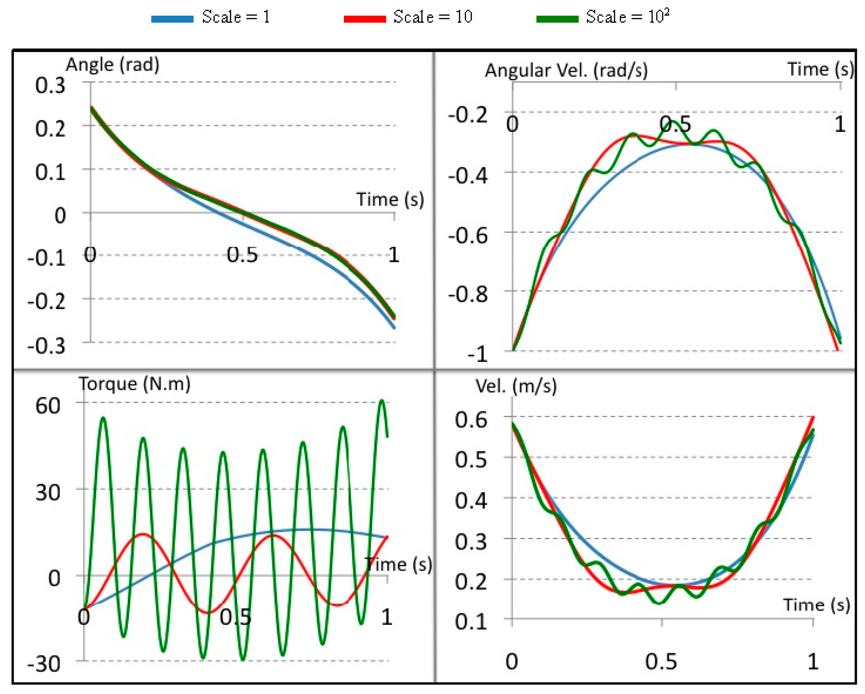
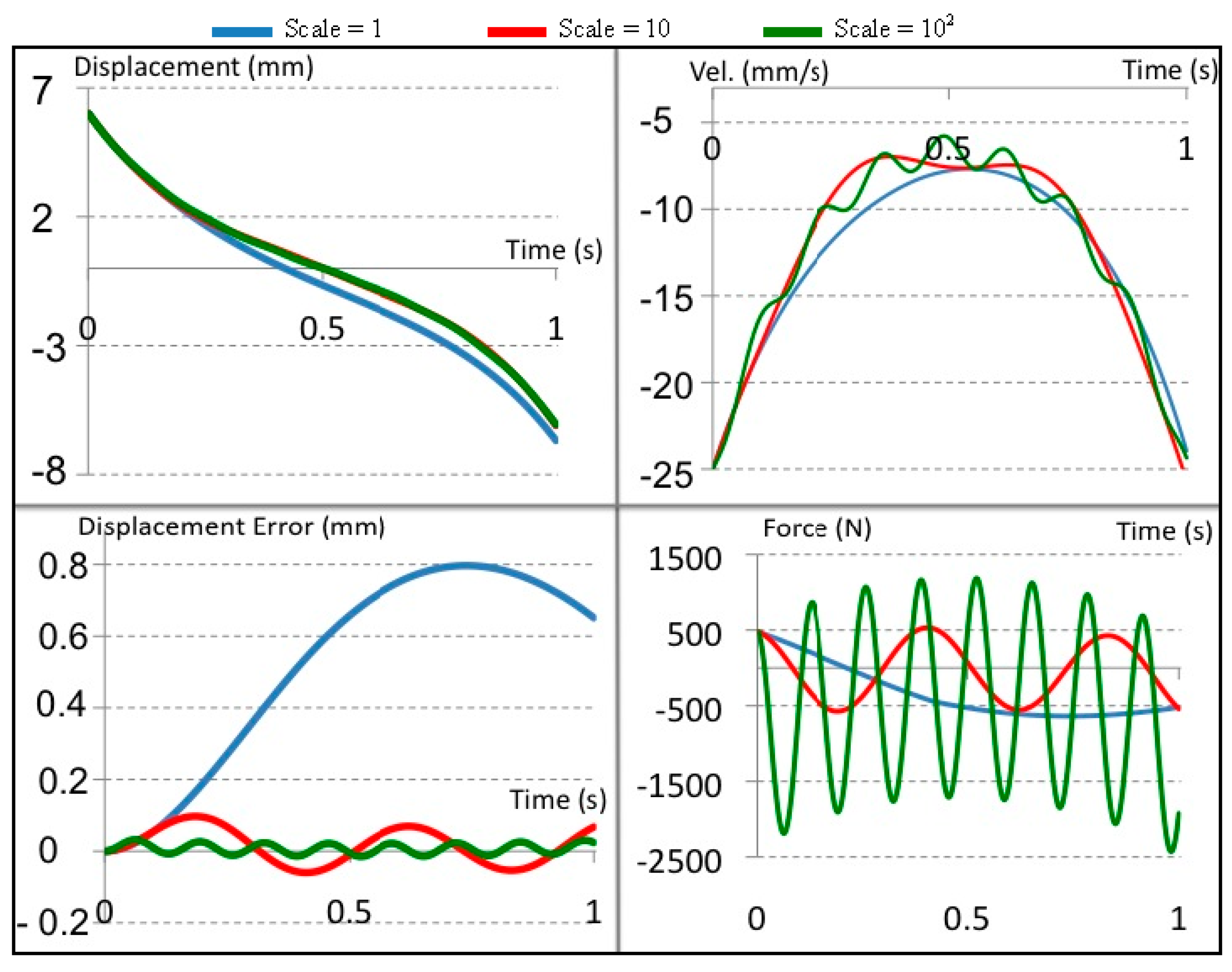
One of the main challenges is the limitation of actuation output force. As it is shown in Figure 29, the force that the DC Motor needs to apply might reach 2.5 kN. It might be too large an amount of applied force for a small size actuator to produce. Even if a rotational motor with a ball screw was used, as we used in our design, the translational speed would have to be very low in order to support such a strong force. It might require a very high rotational speed to move the slide and keep the support of the large force.

Another challenge is to find a suitable spring device. Based on our work in [25], finding a spring in a small size that could have a high stiffness could be difficult. We might need to carefully determine a spring constant value that is suitable for the locomotion characteristic of the bipedal robot.

The mechanical design of such a device might be easy to propose in this paper (see Figure 6), but, practically, it will require many components that do not appear in the basic design. The actuator and the spring sizes might need to be much larger. To assemble so many components with a large size within limited space is a real challenge.

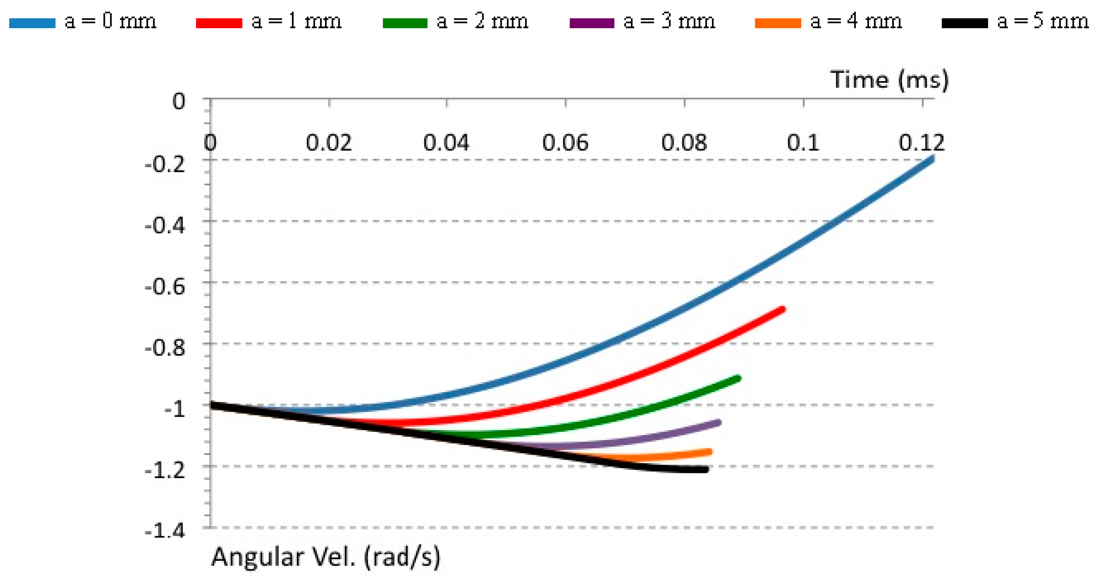
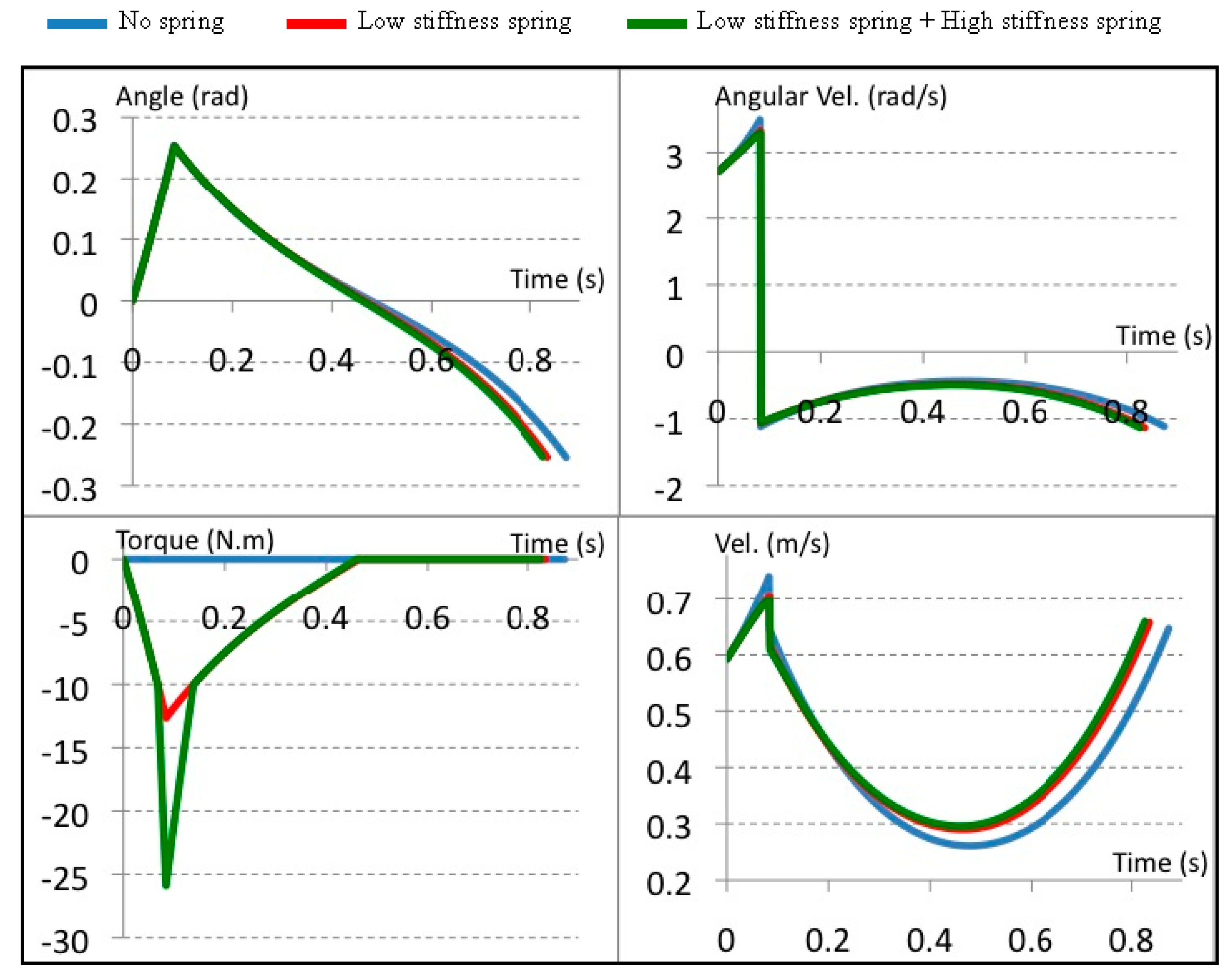
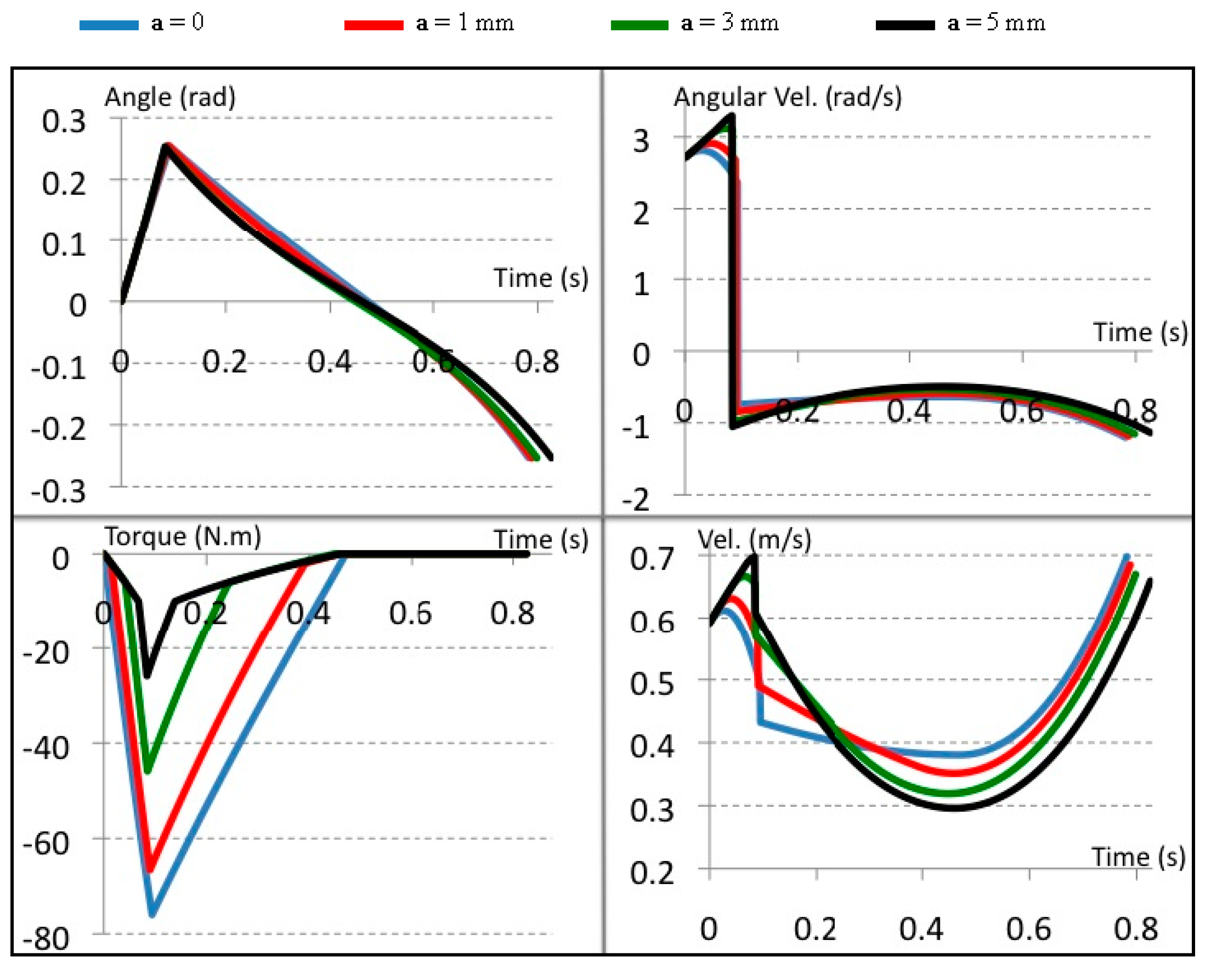
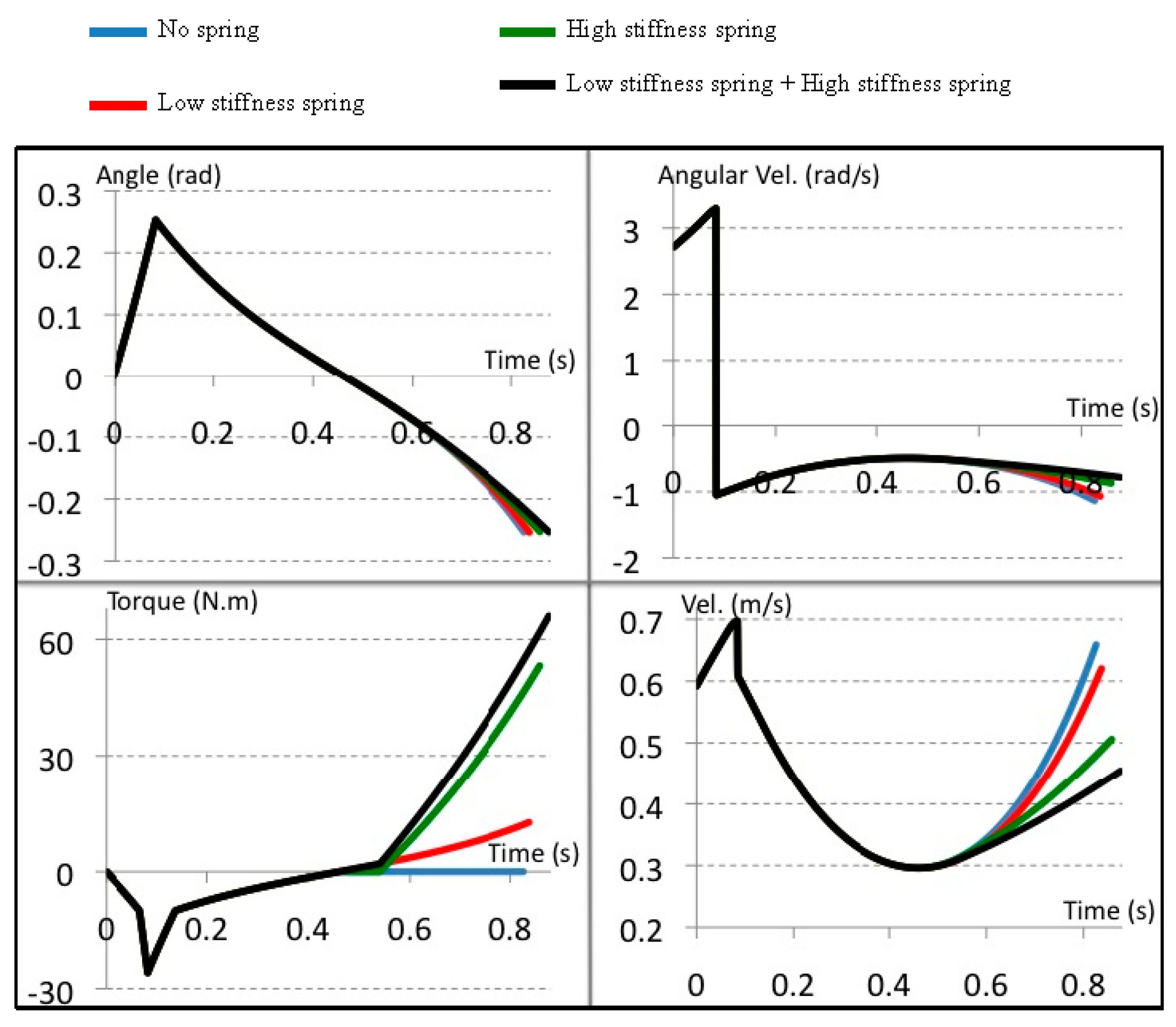
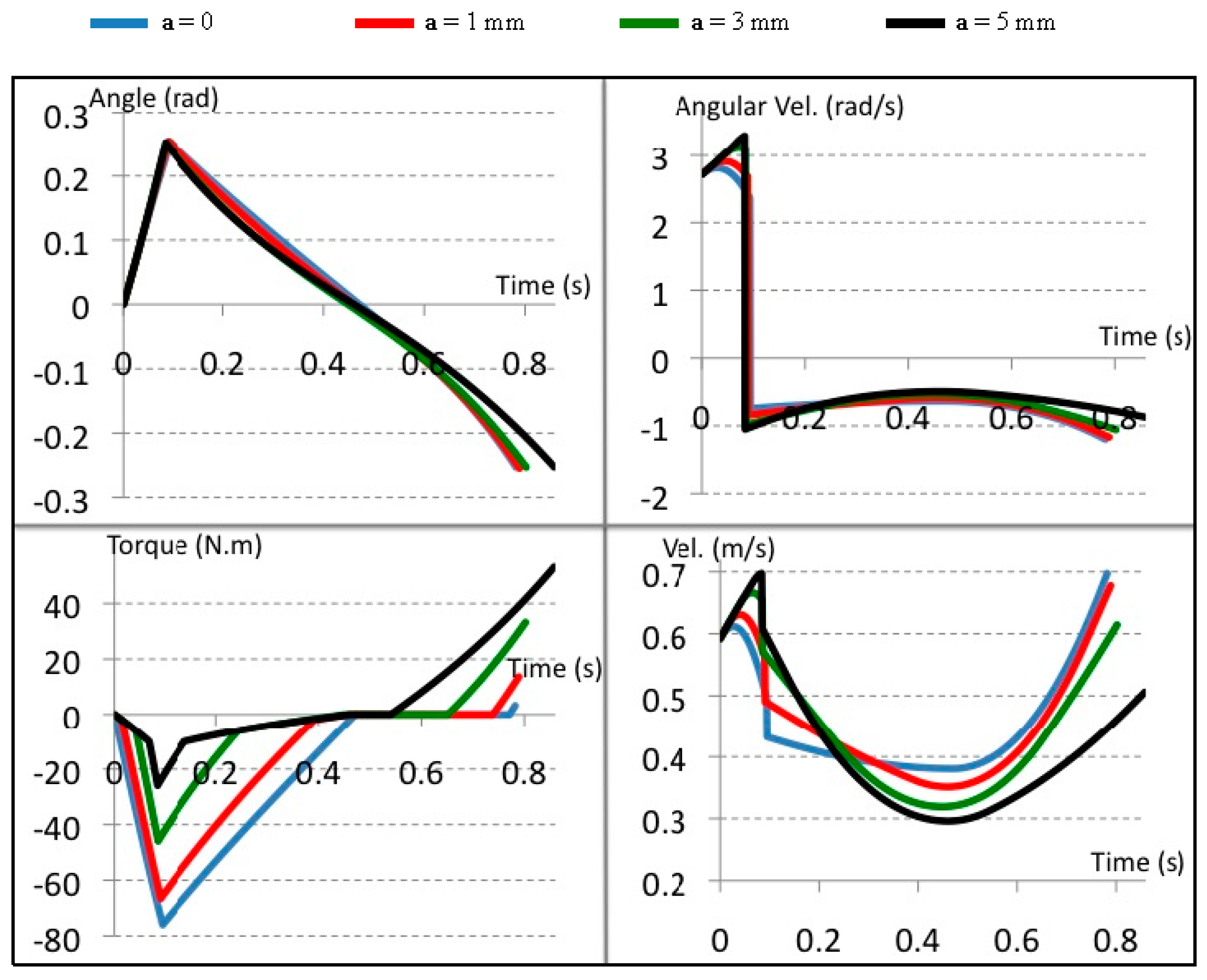
Figure 29. Simulation data for Slider motion during one-step walking in active mode. The data is for 3 experimental tests with different high stiffness scales. Low stiffness spring constant = 80 N/mm. High stiffness spring constant = 400 N/mm. (a) ankle pitch joint angle; (b) ankle pitch joint angular velocity; (c) ankle pitch joint torque; (d) CoM forward velocity.

Figure 29. Simulation data for Slider motion during one-step walking in active mode. The data is for 3 experimental tests with different high stiffness scales. Low stiffness spring constant = 80 N/mm. High stiffness spring constant = 400 N/mm. (a) ankle pitch joint angle; (b) ankle pitch joint angular velocity; (c) ankle pitch joint torque; (d) CoM forward velocity.

Generally, the current study will only provide us with the basic idea for this technique. The implementation of such a technique will require more advanced technology in terms of, say, actuators and materials, that is not currently available. Nevertheless, the current research work presented in this paper could be a helpful guideline for the development of an effective bipedal humanoid robot.

8. Conclusions and Future Work

A new design for a bi-directional adjustable stiffness artificial tendon was introduced in this research work. It was shown that the mechanism could be used to control the rotational motion around the ankle pitch joint. It was also shown that it has the capability of switching between passive and active modes. Several simulation tests were conducted to evaluate the performance of the mechanism based on numerical analysis. The analysis shows that the proposed mechanism design can help to make a motion with a passive joint. However, the analysis of the simulation results led us to the discovery of certain difficulties that would no doubt occur in the actualization of the mechanism and its application to a real robot.

More simulation will be needed to better evaluate the design of the BIASAT. The development of a prototype for this mechanism is an important step toward checking the difficulties of building such a mechanism. Moreover, the testing of it on a real robot should be taken into consideration in order to realize the ability of having a biped robot that can switch between passive and active walking.

References

1. Fukuda, T.; Hasegawa, Y.; Sekiyama, K.; Aoyama, T. Multi-Locomotion Robotic Systems; Springer Berlin Heidelberg: Berlin, Germany; Heidelberg, Germany, 2012. [Google Scholar]
2. Kajita, S.; Hirukawa, H.; Harada, K.; Yokoi, K. Introduction to Humanoid Robotics; Springer: Berlin, Germany; Heidelberg, Germany, 2014. [Google Scholar]
3. Sakagami, Y.; Watanabe, R.; Aoyama, C.; Matsunaga, S.; Higaki, N.; Fujimura, K. The intelligent ASIMO: System overview and integration. In Proceedings of the IEEE/RSJ International Conference on Intelligent Robots and Systems 2002, Piscataway, NJ, USA, 20 September–4 October 2002; pp. 2478–2483.
4. Cho, B.-K.; Kim, J.-H.; Oh, J.-H. Online Balance Controllers for a Hopping and Running Humanoid Robot. Adv. Robot. 2011, 25, 1209–1225. [Google Scholar] [CrossRef]
5. Kajita, S.; Espiau, B. Legged Robots. In Handbook of Robotics; Springer: Berlin, Germany; Heidelberg, Germany, 2008; Part B; pp. 361–389. [Google Scholar]
6. Omer, A.M.M.; Ogura, Y.; Kondo, H.; Morishima, A.; Carbone, G.; Ceccarelli, M.; Lim, H.-O.; Takanishi, A. Development of a Humanoid Robot Having 2-DOF Waist and 2-DOF Trunk. In Proceedings of the Humanoid 2005 Conference, Tsukuba, Japan, 5 December 2005.
7. McGeer, T. Passive dynamic walking. Int. J. Robot. Res. 1990, 9, 62–82. [Google Scholar] [CrossRef]
8. Coleman, M.; Ruina, A. An uncontrolled toy that can walk but cannot stand still. Phys. Rev. Lett. 1998, 80, 3658–3661. [Google Scholar] [CrossRef]
9. Garcia, M.S. Stability, Scaling, and Chaos in Passive Dynamic Gait Models. Ph.D. Thesis, Cornell University, Ithaca, NY, USA, 1999. [Google Scholar]
10. Collins, S.H.; Wisse, M.; Ruina, A. A three-dimensional passive-dynamic walking robot with two legs and knees. Int. J. Robot. Res. 2001, 20, 607–615. [Google Scholar] [CrossRef]
11. Wisse, M.; Frankenhuyzen, J.V. Design and construction of mike; a 2D autonomous biped based on passive dynamic walking. In Adaptive Motion of Animals and Machines; Springer: Tokyo, Japan, 2006; pp. 143–154. [Google Scholar]
12. Cheng, G.; Hyon, S.-H.; Morimoto, J.; Ude, A.; Hale, J.; Colvin, G.; Scroggin, W.; Jacobsen, S. CB: A humanoid research platform for exploring neuroscience. J. Adv. Robot. 2007, 21, 1097–1114. [Google Scholar] [CrossRef]
13. Sugimoto, N.; Morimoto, J.; Hyon, S.-H.; Kawato, M. The eMOSAIC model for humanoid robot control. Neural Netw. 2012, 30, 8–19. [Google Scholar] [CrossRef] [PubMed]
14. Verrelst, B.; van Ham, R.; Vanderborght, B.; Vermeulen, J.; Lefeber, D.; Daerden, F. Exploiting adaptable passive behaviour to influence natural dynamics applied to legged robots. Robotica 2005, 23, 149–158. [Google Scholar] [CrossRef]
15. Vanderborght, B. Dynamic Stabilisation of the Biped Lucy Powered by Actuators with Controllable Stiffness; Springer: Berlin, Germany; Heidelberg, Germany, 2010. [Google Scholar]
16. Wisse, M. Essentials of Dynamic Walking: Analysis and Design of Two-Legged Robots. Ph.D. Thesis, T.U. Delft, Delft, The Netherlands, 2004. [Google Scholar]
17. Dickinson, M.H.; Farley, C.T.; Full, R.J.; Koehl, M.A.R.; Kram, R.; Lehman, S. How Animals Move: An Integrative View. Science 2000, 288, 100–106. [Google Scholar] [CrossRef] [PubMed]
18. Rosenbaum, D.A. Human Motor Control; Academic Press: Cambridge, MA, USA, 2009. [Google Scholar]
19. Winter, D.A. Biomechanics and Motor Control of Human Movement; Wiley: Hoboken, NJ, USA, 2009. [Google Scholar]
20. Ishikawa, M.; Komi, P.V.; Grey, M.J.; Lepola, V.; Bruggemann, G.-P. Muscle-tendon interaction and elastic energy usage in human walking. J. Appl. Physiol. 2005, 99, 603–608. [Google Scholar] [CrossRef] [PubMed]
21. Biewener, A.A.; Farley, C.T.; Roberts, T.J.; Temaner, M. Muscle mechanical advantage of human walking and running: Implications for energy cost. J. Appl. Physiol. 2004, 97, 2266–2274. [Google Scholar] [CrossRef] [PubMed]
22. Omer, A.M.M.; Ghorbani, R.; Lim, H.-O.; Takanishi, A. Simulation of Semi-Passive Dynamic Walking for Humanoid Robots. In Proceedings of the 8th International Conference on Humanoid Robot, Daejeon, Korea, 1–3 December 2008; pp. 541–544.
23. Omer, A.M.M.; Ghorbani, R.; Lim, H.-O.; Takanishi, A. Semi-Passive Dynamic Walking for Biped Walking Robot Using Controllable Joint Stiffness Based on Dynamic Simulation. In Proceedings of the International Conference on Advanced Intelligent Mechatronics, Singapore, 14–17 July 2009; pp. 1600–1605.
24. Omer, A.M.M.; Ghorbani, R.; Lim, H.-O.; Takanishi, A. Simulation based study of a semi-passive dynamic walking for a human size humanoid robot. In Proceedings of the 12th International Conference on Climbing and Walking Robots and the Support Technologies for Mobile Machines, Istanbul, Turkey, 9–11 September 2009; pp. 653–660.
25. Omer, A.; Sulaiman, T.; Ghorbani, R.; Hashimoto, K.; Lim, H.-O.; Takanishi, A. Development of Adjustable Stiffness Mechanism for Bipedal Walking Robot. In Proceedings of the 2nd IFToMM Asian Conference on Mechanism and Machine Science, Tokyo, Japan, 12–14 November 2012. Paper ID 117.
26. Koganezawa, K.; Matsumoto, O. Active/passive hybrid walking by the biped robot TOKAI ROBO-HABILIS 1. In Proceedings of the IEEE/RSJ International Conference on Intelligent Robots and Systems, Lausanne, Switzerland, 30 September–4 November 2002; pp. 2461–2466.
27. Rouse, E.J.; Mooney, L.M.; Herr, H.M. Clutchable series-elastic actuator: Implications for prosthetic knee design. Int. J. Robot. Res. 2014, 33, 1611–1625. [Google Scholar] [CrossRef]