
Trajectory Tracking Control Based on a Composite Disturbance Observer for Unmanned Autonomous Helicopters under Multiple Disturbances

1
College of Automation Engineering, Nanjing University of Aeronautics and Astronautics, Nanjing 211106, China
2
School of Information Science and Technology, Nanjing Forestry University, Nanjing 210037, China
*
Author to whom correspondence should be addressed.
Machines 2024, 12(3), 201; https://doi.org/10.3390/machines12030201
Submission received: 16 January 2024
/
Revised: 14 March 2024
/
Accepted: 16 March 2024
/
Published: 19 March 2024
(This article belongs to the Section Vehicle Engineering)
Abstract
:This paper studies the trajectory tracking anti-disturbance control of unmanned autonomous helicopters (UAHs) under matched disturbances and mismatched ones. Firstly, the six-degrees-of-freedom UAH nonlinear system is simplified via feedback linearization to handle strong coupling, in which the multiple disturbances are composed of modeled disturbances and time-varying bounded ones. Secondly, in order to estimate these disturbances, a new design method of a composite disturbance observer is proposed. On the one hand, for the mismatched disturbances, a normal disturbance observer (DO) combined with a backstepping control are utilized to handle their negative effect. On the other hand, two refined disturbance observers (RDOs) are constructed to estimate the matched disturbances, in which the coupling estimations are involved. Then, by designing two anti-disturbance composite controllers, the boundedness of the tracking errors is guaranteed by using the Lyapunov stability theory. Finally, some numerical simulations are provided to demonstrate the effectiveness and advantage of the proposed control scheme.
1. Introduction
Normally, as a common type of aircraft, unmanned autonomous helicopters (UAHs) have been widely utilized in various industrial and military fields [1,2]. However, the strong coupling and underactuation, cased by strong nonlinearity, have brought great challenges to study the flight control of the UAH. In recent years, research on UAH control systems has achieved a large number of elegant results [1,2,3,4,5]. For instance, in [3], the uncertain terms in the UAH system were approximated via neural networks, and an integral backstepping method combined with a sliding mode control were proposed by considering input saturation. In [4], an adaptive sliding mode fault-tolerant control strategy was proposed for the quadrotor UAV with variable loads, which can compensate for the faults via a neural network approximator. In [5], a flight boundary protection algorithm was presented for the UAH system under uncertainties, by considering the possibility of boundary constraints. However, during the actual flight, the UAHs would be unavoidably affected by the unpredicted disturbances due to unfavorable factors from the UAH system itself to outside environments, which might reduce control performance or even lead to crashing. Yet, some existent control strategies of UAH motions do not wholly consider the influence of complicated outside disturbances. Therefore, how to fully tackle the disturbances and inject their negative effects plays an important role in improving the control performance of UAH systems.
In recent years, anti-disturbance control has drawn much attention from many researchers. In particular, among these proposed methods, because the disturbance observer-based control (DOBC) estimates the disturbance and compensates it in a feedforward manner, it has been widely utilized to tackle anti-disturbance control for UAH systems since it can effectively eliminate the disturbance without sacrificing control performance [6,7,8,9,10,11,12]. It is worth noting that, according to the channel where the disturbance occurs, the disturbances in UAH system can be divided into matched disturbances and mismatched ones. On the one hand, since the matched disturbance exists in the control channel, based on the DOBC method, the disturbance estimation can be directly incorporated into the controller design to eliminate the negative effect. In [6], a nonlinear model predictive controller and disturbance observer (DO) were proposed to derive the optimal performance of UAH trajectory tracking control. In [7], the UAH system was divided into two subsystems, in which the matched disturbance was compensated by using the DOBC approach. In [8], an anti-disturbance feedback controller was designed by treating model uncertainty and disturbance as compounded disturbance and further deriving the estimation by using the DO. On the other hand, since the mismatched disturbance does not exist in the control channel, it cannot be completely suppressed by an anti-disturbance controller. In [9], as for mismatched random disturbance, its influence was suppressed by combining a nonlinear DOBC and feedback control. In [10], a finite-time DO was designed to tackle the mismatched disturbance. In [11,12], the DOBC and backstepping control were combined and utilized to suppress the mismatched disturbance. Meanwhile, owing to complexities of flying environments, the UAH systems may suffer various unfavorable factors. Then, in [13], a composite fault-tolerant control scheme was proposed for a stochastic system under the faults and disturbances, in which random disturbances were modeled as an exogenous system. In [14], a periodic piecewise system suffered from both matched disturbance and a mismatched one, in which a periodic piecewise DO was proposed to estimate the matched disturbance and a performance index was designed to suppress the mismatched one. In [15], a DO design called refined disturbance observer (RDO) was proposed, consisting of the DO and extended state observer (ESO), in which the DO was used to estimate the modeling error and the ESO was exploited to estimate the bounded disturbance. However, except for the faults and modeling errors, these above results aimed to tackle single types of disturbance, such as the norm-bounded disturbance or modeled one. However, based on statistic data and measurable information, only part of the disturbance imposed on the UAH system can be modeled or predicted, while the rest can be regarded as the time-varying bounded one. To the best of our knowledge, few works have considered the anti-disturbance control for the UAH systems under a modeled disturbance and a norm-bounded one, which remains important and challenging.
Meanwhile, as for the UAH systems, many existent control methods have been established based on approximate linearized systems and linear control techniques, such as PID control [16,17], LQR control [18,19], and control [20,21]. Normally, the linearized UAH systems cannot accurately describe all the motions of the UAH system, and the linear control approaches cannot meet the high robust requirements in practice. Yet, the nonlinearity and underactuation of the UAH system lead to significant challenges in proposing the control strategy. In order to solve this problem, a new feedback linearization method was proposed to simplify the nonlinear UAH systems. In [22,23], the approximate feedback linearization method was used to simplify the UAH system by choosing the outputs as the position and yaw angles. In [24,25], the UAH system was simplified by applying the feedback linearization to tackle the heave dynamics and decouple the roll with pitch dynamics. Meanwhile, since the backstepping method can be utilized to control uncertain control systems, it was widely utilized to analyze the control issue of UAH systems. In [26], an adaptive neural network backstepping control scheme was proposed for the UAH system. In [27], the optimal control and backstepping control were combined to study the tracking control for the UAH system. In [28], a feedforward–feedback composite control scheme was proposed based on the generalized PI observer and backstepping control. However, as for the full degree-of-freedom UAH system, initially, since it processes underactuation, strong coupling, high orders, and nonlinearity, a feedback linearization method needs to be proposed to simplify the nonlinear UAH system by selecting suitable outputs and involving multiple disturbances; secondly, as for the anti-disturbance control for the simplified UAH system, some improvements on existent DOBC methods need to be imposed since multiple disturbances are involved, which can further combine a backstepping control to the present controller design.
Motivated by the above discussions, by exploiting an improved DOBC method, feedback linearization, and backstepping control, this work investigates the tracking control for the 6-DOF UAH system under multiple disturbances. The main contributions of this work are listed as follows:
- In practice, the UAH always suffers from different types of outside disturbances. Then, as for the simplified UAH system under matched disturbances and mismatched ones, based on the statistic data and experiences, the disturbances are divided into the modeled parts and the bounded time-variable ones. In order to derive the estimations, a composite observer design strategy is initially proposed, in which the normal DO is utilized to estimate the mismatched disturbance, and the improved RDOs are exploited to estimate the matched disturbance including the modeled part and the bounded one. In comparison with some existent works, our proposed disturbance observer can be more effective in tackling more complicated disturbances.
- Based on above estimations and tracking control target, the backstepping control approach is employed to reject the mismatched disturbance, while as for the matched disturbances, two anti-disturbance composite controllers are put forward to reject these disturbances and ensure that the UAH tracks the reference signals. Then, a co-design method of the observer gains and controller ones are established in terms of a set of inequalities. Therefore, by choosing suitable parameters, our proposed control scheme can not only compensate for outside disturbances, but also guarantee that tracking errors are in a reasonable range, as small as possible.
The mathematical model of UAH system and some preliminaries are presented in Section 2. Section 3 states related works about anti-disturbance control for the UAH system. Section 4 introduces approximate feedback linearization model of UAH system. The anti-disturbance backstepping controller is designed in Section 5. The simulation experiments are conducted in Section 6 to demonstrate the feasibility of the proposed methods. Finally, Section 7 states our conclusions.
Notation 1.
I is an identity matrix with appropriate dimensions. , , and are the abbreviations of trigonometric functions , , and , respectively. denotes the rth order time derivative of the function . represents the Euclidean norm for a matrix A. represents the eigenvalues of the matrix (A).
2. Problem Formulation and Preliminaries
In this section, the 6-DOF UAH nonlinear system is described, based on which a simplified UAH system under multiple disturbances is established via a feedback linearization method. In what follows, the problem formulations and preliminaries are presented.
2.1. Problem Formulations
The UAH model in this work mainly involves the ground coordinate system and the aircraft coordinate system, whose coordinate axis is shown in Figure 1. Based on this figure, we consider the 6-DOF model for the UAH system [29], described as follows:
where and represent the position vector and velocity vector in the inertial frame, respectively; is a unitary vector, m is the mass of the UAH, g is the gravitational acceleration; and represent the Euler angle vector and the angular rate one in the body frame, respectively. represents the collective pitch of the UAH, and denotes the control input vector. and satisfy the term , where is the main rotor thrust, and satisfy the term , where is the moment vector. denotes the inertia matrix. The rotation matrix from the body frame to the inertial frame is defined as
where , , and denote the roll angle, pitch angle and yaw angle, respectively; , , and represent the roll angular rate, pitch angular rate and yaw angular rate, respectively; and represent the Euler angle vector and the angular velocity one. The attitude kinematic matrix is defined as
and the derivative of is presented as
where the is given as follows:
2.2. Preliminaries
Assumption 1
([5]). During the UAH flying procedure, the pitch angle and roll angle need to satisfy and .
Lemma 1
([9]). For any scalars , , and given vectors x and y with appropriate dimensions, the inequality holds
where .
Remark 1.
Throughout the flight process, the roll angle and the pitch angle cannot cross the interval for the UAH system; otherwise, it would be overturned. On the other hand, from the UAH system model, the angles meet the above condition to make the matrices and nonsingular. Thus, Assumption 1 is reasonable in practice.
3. Related Works
The main focus of this work aims to study the anti-disturbance control for the UAH system under outside disturbances based on the combination of DOBC and backstepping control. The problem can be divided into two aspects: the suppression of multiple types of outside disturbances and the design of the tracking controller for the UAH system. In terms of anti-disturbance control under multiple disturbances, Ref. [13] proposed a fault-tolerant control scheme for stochastic systems under faults and disturbances, which did not involve the disturbance estimation. Ref. [14] exploited the disturbance observer to estimate the matched disturbance and used the performance index to suppress the mismatched one. Yet, as for the anti-disturbance issues in UAH systems, most existent control schemes based on the DOBC method paid much research attention to single type of the disturbance. That is to say, some works aimed to investigate the time-variable bounded disturbances, while the others assumed that the disturbance was strictly generated by an outside system based on the assumption that the information about the disturbance is exactly known [9,22,23,26,27,28]. It is worth noting that, owing to the complexities of flying environments, only part of the data of outside disturbance can be measured and counted, which can be modeled as an exogenous system, while the rest cannot be modeled but satisfies the bounded time-varying condition. Therefore, it is more practical and significant to investigate the anti-disturbance control for the UAH system under multiple types of disturbances.
4. Approximate Feedback Linearization Model of UAH System
The control target of this work aims to guarantee that the UAH tracks the desired position and the yaw angle . The exact input–output linearization cannot linearize the whole system. Thus, the approximate feedback linearization technique is utilized to simplify the UAH system (1). Based on [10], two variables and are introduced to guarantee that the UAH system can be linearized with the input–output feedback linearization method. Then, the UAH system (1) is rewritten as [10]:
where the term is replaced by the main rotor thrust . Let and be inputs, and choose and as outputs. The relative degree of the system (5) is , and its dimension is , namely , which means that the system (5) can be transformed into a new system. One new control input is defined, where .
By exploiting the feedback linearization method in [10] and considering the existence of multiple disturbances, the simplified UAH system can be further written as
where , , , , , , and . Disturbances , , and are described by using an exogenous system, while and are time-varying bounded ones. Then, partial variables are given as
Assumption 2
([15]). The modeled disturbances are described by the following exogenous model:
where is the internal variable. and are the known matrices with appropriate dimensions.
Assumption 3
([13]). The time-varying bounded disturbances and are differentiable, i.e.,
where is unknown but bounded; that is to say, there exist positive constants and such that
Assumption 4
([30]). The parameter matrices and for any make observable, where .
Remark 2.
In practical flight, the disturbances imposing on the UAH system are complicated and unpredictable. Yet, based on available information and statistical data, part of the disturbances can be described by using the outside model, while the rest of the disturbances, although they cannot be modeled, typically satisfy the time-varying bounded condition. Yet, as for the anti-disturbance issue on the UAH system, most existent works have treated the outside disturbance as a unified one and proposed a normal DO or an ESO to derive the estimation and execute the compensation [6,7,8,9,10,11,12], which is available but not effective enough. Therefore, it is more reasonable and meaningful to estimate the disturbances for UAV systems by designing the composite disturbance observers (CBOs), which can greatly improve the efficiency of the compensation and tracking performance [15].
In order to facilitate forthcoming discussions, as for UAH systems (6), this work only considers the situation that the matched disturbances include two types of disturbances, while the mismatched disturbance only consists of the modeled one. Then, in what follows, the DO and backstepping control are combined to handle the mismatched disturbance , while the CBO based backstepping control is exploited to tackle the disturbances , , , and . The designing process of the anti-disturbance flight controller is shown as a diagram in Figure 2.
5. Composite Disturbance Observer and Flight Controller of the UAH System
5.1. Anti-Disturbance Backstepping Controller Based on Disturbance Observer
We define the tracking variables and as
where and are the virtual control laws in the form of
where denotes the controller parameter. Then, we choose one Lyapunov function for as
According to (9)–(12), the derivative of (13) is presented as
We define the tracking variable as
where is the virtual control law designed as
where denotes the controller parameter, and is the estimation of , which will be compensated by using . The disturbance observer of is built as
where is the estimation of , is an auxiliary variable, and denotes the observer gain. Defining the error vector , the derivative of can be obtained as
We choose the Lyapunov function concerning as
The derivative of (19) is obtained from (15), (16), and (18):
5.2. Anti-Disturbance Backstepping Controller Based on Refined Disturbance Observer
We define the tracking variable as
where is the virtual control law and expressed as
where denotes the virtual controller parameter. We choose the Lyapunov function on as
In view of (22), the derivative of (23) is obtained as
From the dynamics , the controller can be designed as
where the controller parameter , and and are the estimations of and , respectively. To estimate the disturbances and , a refined disturbance observer (RDO) based on the CBO and state observer is designed as
where and are the estimations of and , respectively; is the auxiliary variable; , , and are the gains of the RDO. Defining the error vectors , , and , the dynamics of their derivatives are obtained as
We define as the error vector of the RDO. According to (27)–(29), the derivative of is expressed as
where the matrix parameters are denoted as
Then, we choose the Lyapunov function concerning as
where is a definitely positive matrix of suitable dimensions. According to (25) and (30), the derivative of (31) is given by
We define the variables and as
where and are the virtual control laws represented by
with representing the controller parameter. We choose the Lyapunov function concerning as
Then, the derivative of (37) is given by
From the dynamics , the controller is designed as
where the controller parameter , and and are the estimations of and , respectively. To estimate the disturbances and , another RDO is built as follows:
where and are the estimations of and , respectively; is the auxiliary variable; , , and are the gains of the RDO. We define the error vectors , , and . The derivatives of these observer errors are obtained as
We define as the error vector. According to (41)–(43), the derivative of is expressed as
where the matrix parameters are organized as
We choose the Lyapunov function on as
where is a definitely positive matrix of appropriate dimensions. According to (39) and (44), the derivative of (46) is given by
5.3. Stability Analysis
In this subsection, a stability criterion is summarized in the following theorem. Based on the combination of the approximate feedback linearization, backstepping control, and refined disturbance observer including the DO and CDO, the tracking errors can be restricted within the reasonable range, i.e., the UAH system (1) can track the predefined signals of the position and yaw angles.
Theorem 1.
Consider the UAH system (6) under multiple disturbances, including the modeled disturbance (7) and the bounded one (8). Design the controllers in (25) and (39), the disturbance observer (17), and the refined disturbance observers in (26) and (40). The tracking errors for the UAH system are uniformly bounded in the reasonable small range, if there exist suitable matrices , and constants , such that the following inequalities hold:
Proof.
Based on (13), (19), (23), (31), (37), and (46), we define an augmented Lyapunov function as
Combining (14), (20), (24), (32), (38), and (47), the derivative of (48) is expressed as
In view of Lemma 1, the following inequalities can be deduced:
We choose the suitable matrix such that the term is a Hurwitz formula, and the following inequality is true:
where . On the other hand, there exist the suitable constants , , , , , and , such that the following inequalities hold:
Hence, the derivative of can be rewritten as
where
Then, (51) can be obtained as
where
In summary, the tracking errors are uniformly bounded, and this completes the proof. □
Remark 3.
Based on the Lyapunov stability theory, Theorem 1 can ensure that the trajectory tracking error is uniformly bounded within a reasonable small range. However, in some typical control targets, the bounded tracking error for the UAH flight cannot meet the practical requirements when the tracking accuracy is highly demanded. Then, if the derivatives of the disturbances are satisfied to be energy-bounded, the tracking error can asymptotically converge to zero by combining the proof of Theorem 1 and control.
6. Simulated Example
In this section, some simulations are provided to demonstrate the effectiveness of the proposed control strategy. During the simulation, the hardware environment for this experiment was DESKTOP-BCQI0VS, which was made by ASUS from China, and the processor was the 11th Gen Intel Core i7-11700 with 2.50 GHz. The simulation was conducted on MATLAB R2021a and Simulink integrated with MATLAB R2021a.The related parameters that the UAH system can refer to [29], are given as follows:
Since the tracking target is studied in this work, the anti-disturbance controller needs to ensure that the UAH system tracks the desired position and the yaw angles. Then, the desired signals are given as
and the initial values of the UAH system are selected as and . On the other hand, the parameters of the exogenous models describing the disturbances , , and are presented as follows:
The time-varying bounded disturbances and are presented as follows:
Moreover, the controller gains are selected as , and . According to Theorem 1, the the DO and RDO gains can be chosen as
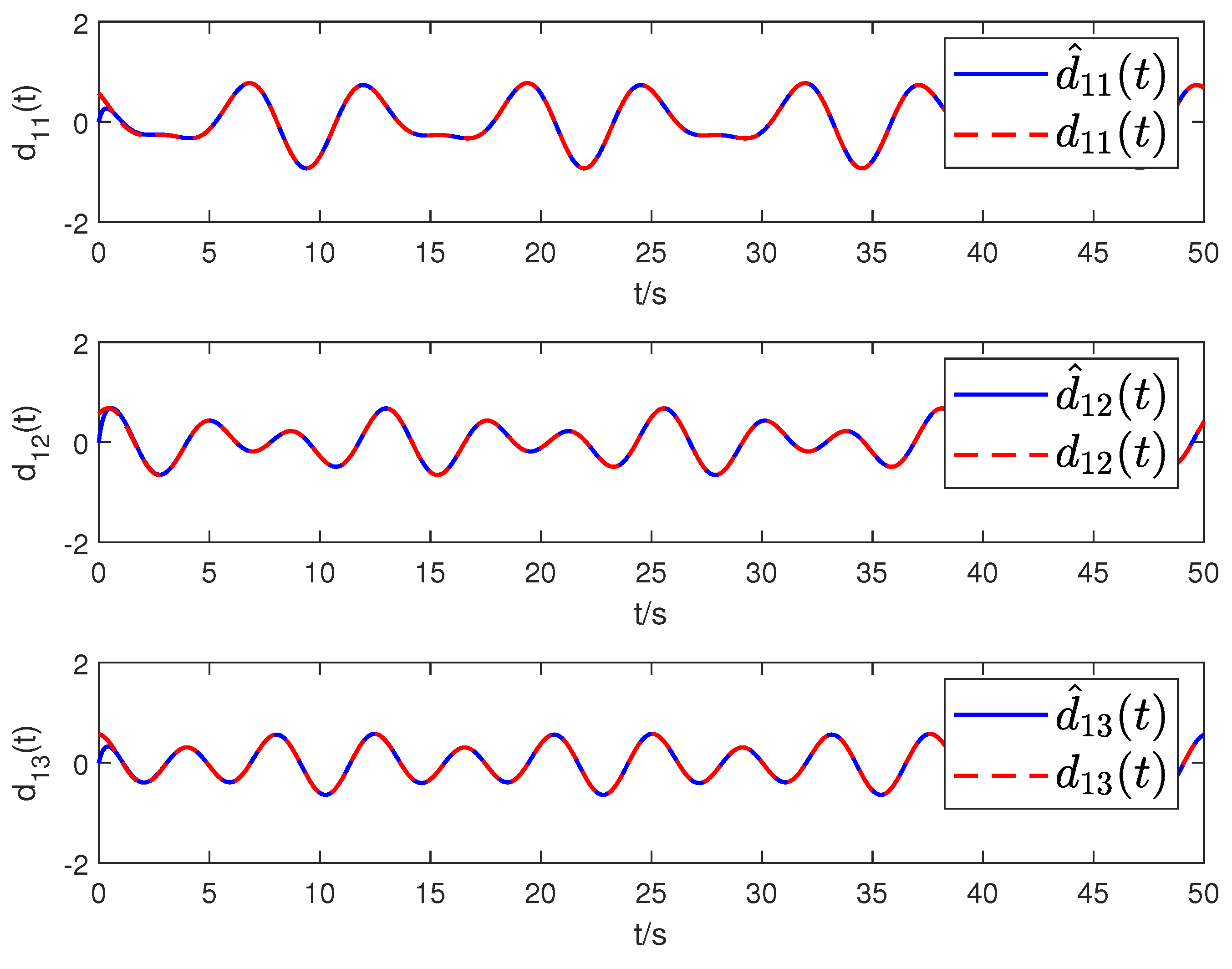
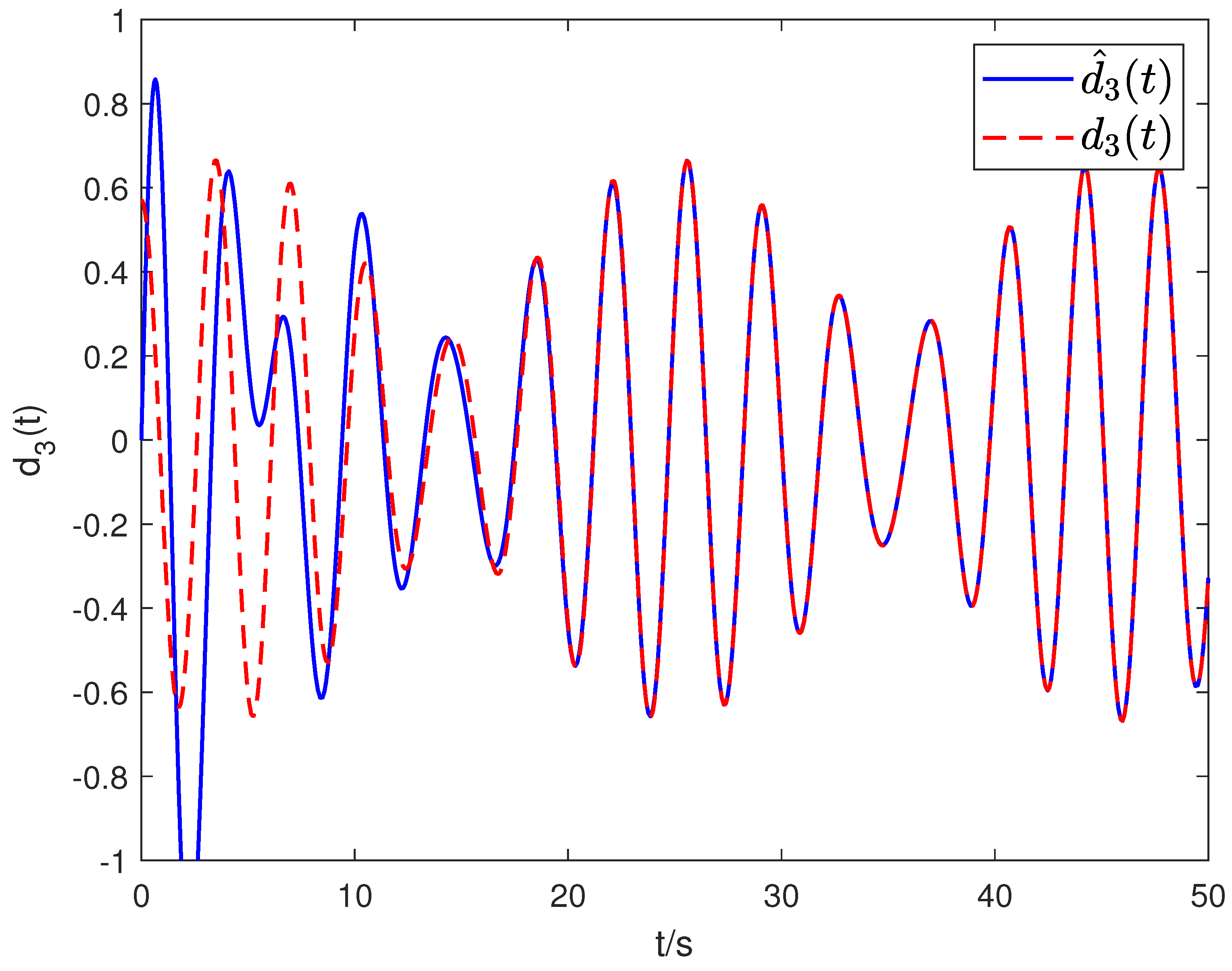
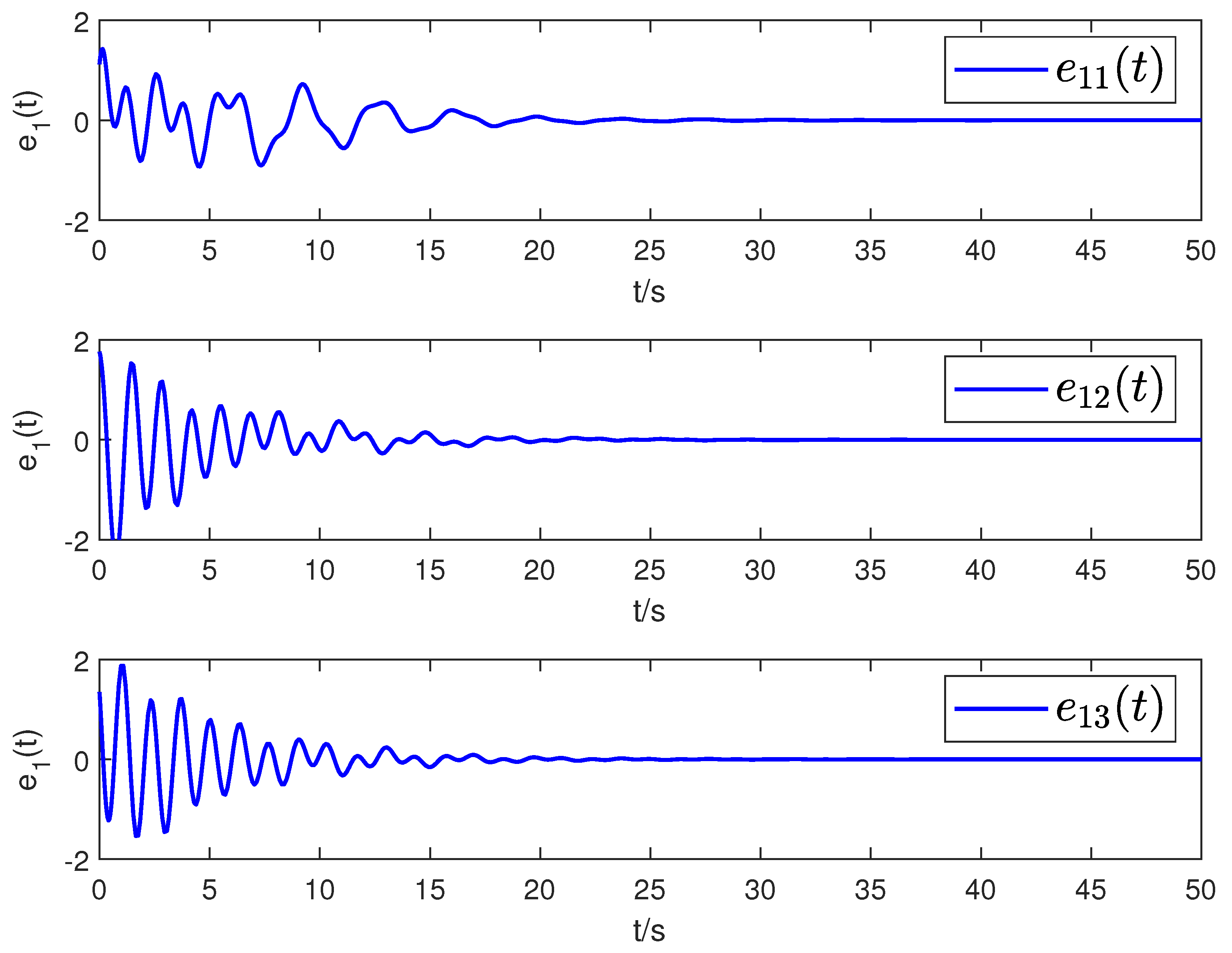
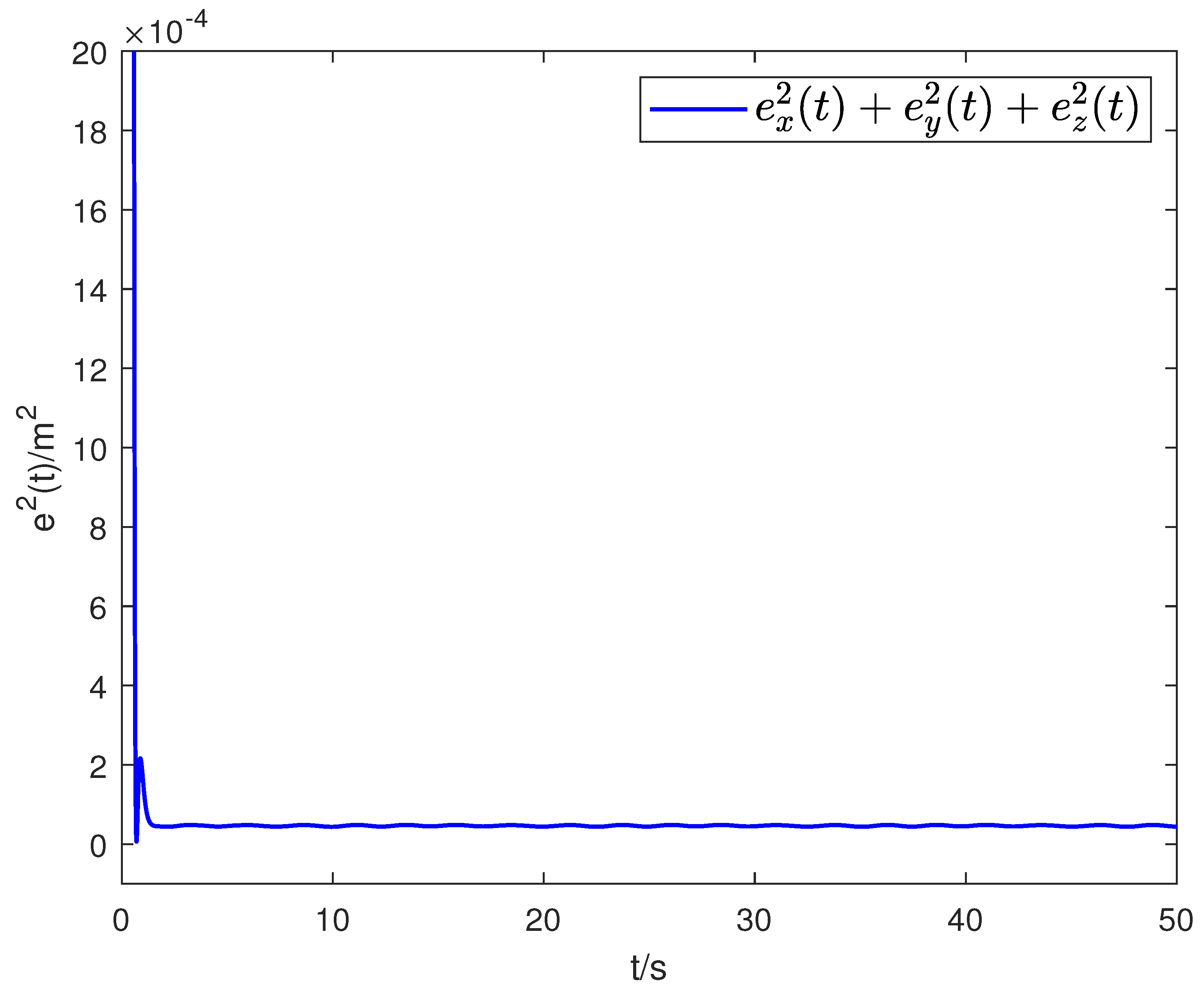
The simulated results are presented in Figure 3, Figure 4, Figure 5, Figure 6, Figure 7, Figure 8, Figure 9, Figure 10, Figure 11, Figure 12, Figure 13, Figure 14 and Figure 15. The modeled disturbances and their estimations are shown in Figure 3, Figure 4 and Figure 5, while the time-variable bounded disturbances with their estimations are presented in Figure 6 and Figure 7. Based on these figures, it is verified that these disturbances can be effectively estimated, which is further supported by the estimating errors in Figure 8 and Figure 9. In Figure 8 and Figure 9, the estimation errors and are converge to zero over time. Except for the disturbance estimations, we further give some simulations on the UAH states and tracking errors, from which not only the effectiveness but also the superiority can be presented to verify our proposed scheme. Initially, for convenience, we denote the position tracking error and the tracking error of yaw angle as follows:
Then, by using the RDO-based controller in this work, the simulations in Figure 10, Figure 11, Figure 12 and Figure 13 show that the responses of the position and the yaw angle can track the desired signals, which can be further checked in Figure 14. Moreover, in order to show the advantages of our designed controller based on the RDO and DO, we also utilized the DOBC method to obtain the anti-disturbance tracking controller, in which the disturbances are regarded as the unified ones. From the Figure 10, Figure 11, Figure 12, Figure 13, Figure 14 and Figure 15, it can be verified that the tracking performance by the RDOBC is much better than the one by the DOBC, which means that our methods can achieve higher tracking efficiency in terms of smaller amplitude and better stability.
Now, in order to further compare our method with the DOBC in [10], based on the Figure 10, Figure 11, Figure 12 and Figure 13, we chose two typical moments () to derive exact values of the tracking errors, which are summarized in Table 1. From this table, on the one hand, at , the values of the tracking errors obtained by our method are , and , while the ones of the tracking errors obtained by the DOBC in [10] are derived as and . On the other hand, when , the values of the tracking errors obtained by our method are given as and , while the ones of the tracking errors obtained by the DOBC in [10] are computed as and . Then, based on Table 1, no matter whether or , the tracking efficiency achieved by our method is significantly higher than the one by the DOBC method in [10], which further demonstrates the superiority of our proposed method. Moreover, we provide some comparisons based on mean squared errors (MSEs) to further highlight our control scheme, as shown in Table 2. From Table 2, our method still obtain much smaller MSEs than that of the DOBC, indicating that our approach achieves better tracking performance.
Meanwhile, since the term is included into the observers in (26), it means that the estimations of do not only depend on the main rotor thrust , but also need its time derivative . However, in practical situations, when using sensors to collect the information on main rotor thrust and its derivative, it is inevitable that the measurement noises are existent. These noise effects will directly impact the estimation accuracy of the observers in (26), thereby affecting the tracking performance of the UAH system. In order to further illustrate the results of this work, based on above selected parameters, it was assumed that the sensor measurements are affected by white noise with its power ranging from . The simulation results are shown in Figure 16 and Figure 17 to illustrate our proposed observer and controller. From Figure 16 and Figure 17, despite being influenced by the white noise, even though the estimation error in Figure 16 and the tracking error in Figure 17 exhibit oscillations, they are still limited within reasonable small ranges, indicating that the observer and controller proposed in this work still remain effective.
7. Conclusions
In this work, the issue of trajectory tracking control has been investigated for full degree-of-freedom UAH systems under multiple disturbances. Firstly, in order to simplify the procedure of controller design, an approximate feedback linearization method was adopted to simplify the nonlinear UAH system. Secondly, two types of disturbance observers were utilized to describe the mismatched disturbance and matched ones, in which the matched disturbances were divided into the modeled part and the variable-bounded one. Thirdly, an anti-disturbance trajectory tracking controller was proposed on the basis of backstepping control and disturbance estimations, which can ensure the bounded stability of the tracking error. Finally, some simulations and comparisons were conducted to demonstrate the proposed control strategy.
Based on the proposed methods in this work, some illustrations are presented in what follows. Initially, as for quantitative analysis, our control scheme can achieve better efficiency of tracking errors by increasing multiple percentages at and when compared with the ones obtained by the DOBC method; secondly, the advantage of our control scheme mainly depends on the division of outside disturbances into the modeled part and bounded one; a new design of a composite DO was presented to derive tighter estimations and an effective tracking controller was proposed; thirdly, the disadvantage of our methods includes the lack of good robustness, since the parameter uncertainties and modeling error are not involved; fourthly, the limitation of this work manifests in the fact that our anti-disturbance scheme can only tackle the disturbances with simple characteristics, while more complicated ones cannot be dealt with, such as strong airflow, strong gusts, wind shear, and turbulence. Therefore, in the future, we will investigate the issue of anti-disturbance control for the UAH system under more complicated disturbances, such as jumping disturbances, stochastic disturbances, and so on.
Author Contributions
Conceptualization, S.P. and T.W.; methodology, S.P.; software, S.P.; validation, S.P., T.W., H.Z. and T.L.; formal analysis, T.W. and H.Z.; investigation, T.W. and H.Z.; writing—original draft preparation, S.P.; writing—review and editing, H.Z. and T.L. All authors have read and agreed to the published version of the manuscript.
Funding
This work was supported by the National Natural Science Foundations of China (Nos. 62073164, 61922042), Aeronautical Science Foundation of China (No. 2023Z032052001), and Project of Graduate Research and Practice Innovation of Nanjing University of Aeronautics and Astronautics (No. xcxjh20230319).
Data Availability Statement
The datasets generated during the current work are available from the corresponding author on reasonable request.
Conflicts of Interest
The authors declare no conflicts of interest.
References
- Wu, B.; Wu, J.; He, W.; Tang, G.; Zhao, Z. Adaptive neural control for an uncertain 2-DOF helicopter system with unknown control direction and actuator faults. Mathematics 2022, 10, 4342. [Google Scholar] [CrossRef]
- Hachiya, D.; Mas, E.; Koshimura, S. A reinforcement learning model of multiple UAVs for transporting emergency relief supplies. Appl. Sci. 2022, 12, 10427. [Google Scholar] [CrossRef]
- Wan, M.; Chen, M.; Lungu, M. Integral backstepping sliding mode control for unmanned autonomous helicopters based on neural networks. Drones 2023, 7, 154. [Google Scholar] [CrossRef]
- Yang, P.; Wang, Z.; Zhang, Z.; Hu, X. Sliding mode fault tolerant control for a quadrotor with varying load and actuator fault. Actuators 2021, 10, 323. [Google Scholar] [CrossRef]
- Ma, H.; Chen, M.; Feng, G.; Wu, Q. Disturbance-observer-based adaptive fuzzy tracking control for unmanned autonomous helicopter with flight boundary constraints. IEEE Trans. Fuzzy Syst. 2023, 31, 184–198. [Google Scholar] [CrossRef]
- Liu, C.; Chen, W.; Andrews, J. Tracking control of small-scale helicopters using explicit nonlinear MPC augmented with disturbance observers. Control Eng. Pract. 2012, 20, 258–268. [Google Scholar] [CrossRef]
- Ullah, I.; Pei, H. Sliding mode tracking control for unmanned helicopter using extended disturbance observer. Arch. Control Sci. 2019, 29, 169–199. [Google Scholar]
- He, Y.; Pei, H.; Sun, T. Robust tracking control of helicopters using backstepping with disturbance observers. Asian J. Control 2014, 16, 1387–1402. [Google Scholar] [CrossRef]
- Li, Y.; Chen, M.; Shi, P.; Li, T. Stochastic anti-disturbance flight control for helicopter systems with switching disturbances under markovian parameters. IEEE Trans. Aerosp. Electron. Syst. 2022, in press. [Google Scholar] [CrossRef]
- Chen, L.; Li, T.; Liu, L.; Mao, Z. Trajectory tracking anti-disturbance control for unmanned aerial helicopter based on disturbance characterization index. Control Theory Technol. 2023, in press. [Google Scholar] [CrossRef]
- Zhou, L.; Jiang, F.; She, J.; Zhang, Z. Generalized-extended-state-observer-based repetitive control for DC motor servo system with mismatched disturbances. Int. J. Control Autom. Syst. 2020, 18, 1936–1945. [Google Scholar] [CrossRef]
- Yang, J.; Zolotas, A.; Chen, W.; Michal, K.; Li, S. Robust control of nonlinear MAGLEV suspension system with mismatched uncertainties via DOBC approach. ISA Trans. 2011, 50, 389–396. [Google Scholar] [CrossRef]
- Sun, S.; Wei, X.; Zhang, H.; Karimi, H.; Han, J. Composite fault-tolerant control with disturbance observer for stochastic systems with multiple disturbances. J. Frankl. Inst. 2018, 355, 4897–4915. [Google Scholar] [CrossRef]
- Aravinth, N.; Satheesh, T.; Sakthivel, R.; Ran, G.; Mohammadzadeh, A. Input-output finite-time stabilization of periodic piecewise systems with multiple disturbances. Appl. Math. Comput. 2023, 453, 128080. [Google Scholar] [CrossRef]
- Cui, Y.; Qiao, J.; Zhu, Y.; Yu, X.; Guo, L. Velocity-tracking control based on refined disturbance observer for gimbal servo system with multiple disturbances. IEEE Trans. Ind. Electron. 2022, 69, 10311–10321. [Google Scholar] [CrossRef]
- Azarmi, R.; Tarvakoli-Kakhki, M.; Fatehi, A. Analytical design of fractional order PID controllers based on the fractional set-point weighted structure: Case study in twin rotor helicopter. Mechatronics 2015, 31, 222–233. [Google Scholar] [CrossRef]
- Mary, A.; Miry, A.; Miry, M. Design robust H-infinity-PID controller for a helicopter system using sequential quadratic programming algorithm. J. Chin. Inst. Eng. 2022, 45, 688–696. [Google Scholar] [CrossRef]
- Liu, L.; Chen, M.; Li, T. Disturbance observer-based LQR tracking control for unmanned autonomous helicopter slung-load system. Int. J. Control Autom. Syst. 2022, 20, 1166–1178. [Google Scholar] [CrossRef]
- Zhang, J.; Yang, Y.; Zhao, Z.; Hong, K. Adaptive neural network control of a 2-DOF helicopter system with input saturation. Int. J. Control Autom. Syst. 2022, 21, 318–327. [Google Scholar] [CrossRef]
- Chen, J.; He, C. Modeling, Fault detection, and fault-tolerant control for nonlinear singularly perturbed systems with actuator faults and external disturbances. IEEE Trans. Fuzzy Syst. 2022, 30, 3009–3022. [Google Scholar] [CrossRef]
- Wang, X.; Lu, G.; Zhong, Y. Robust H-infinity attitude control of a laboratory helicopter. Robot. Auton. Syst. 2013, 61, 1247–1257. [Google Scholar] [CrossRef]
- Koo, T.; Sastry, S. Output tracking control design of a helicopter model based on approximate linearization. In Proceedings of the 37th IEEE Conference on Decision and Control, Tampa, FL, USA, 16–18 December 1998; Volume 4, pp. 3635–3640. [Google Scholar]
- Koo, T.; Sastry, S. Differential flatness based full authority helicopter control design. In Proceedings of the 38th IEEE Conference on Decision and Control, Phoenix, AZ, USA, 7–10 December 1999; Volume 2, pp. 1982–1987. [Google Scholar]
- Song, B.; Liu, Y.; Fan, C. Feedback linearization of the nonlinear model of a small-scale helicopter. J. Control Theory Appl. 2010, 8, 301–308. [Google Scholar] [CrossRef]
- Xin, Y.; Qin, Z.; Sun, J. Input-output tracking control of a 2-DOF laboratory helicopter with improved algebraic differential estimation. Mech. Syst. Signal Process. 2019, 116, 843–857. [Google Scholar] [CrossRef]
- Yang, Y.; Zheng, X. Adaptive NN backstepping control design for a 3-DOF helicopter: Theory and experiments. IEEE Trans. Ind. Electron. 2020, 67, 3967–3979. [Google Scholar] [CrossRef]
- Glida, H.; Abdou, L.; Chelihi, A.; Sentouh, C.; Hasseni, S. Optimal model-free backstepping control for a quadrotor helicopter. Nonlinear Dyn. 2020, 100, 3449–3468. [Google Scholar] [CrossRef]
- Wang, X.; Yu, X.; Li, S.; Liu, J. Composite block backstepping trajectory tracking control for disturbed unmanned helicopters. Aerosp. Sci. Technol. 2019, 85, 386–398. [Google Scholar] [CrossRef]
- Fang, X.; Wu, A.; Shang, Y.; Dong, B. Robust control of small-scale unmanned helicopter with matched and mismatched disturbances. J. Frankl. Inst. 2016, 353, 4803–4820. [Google Scholar] [CrossRef]
- Li, Y.; Chen, M.; Li, T.; Wang, H. Robust resilient control based on multi-approximator for the uncertain turbofan system with unmeasured states and disturbances. IEEE Trans. Syst. Man Cybern. Syst. 2016, 353, 4803–4820. [Google Scholar] [CrossRef]
Figure 1.
UAH system coordinate axis.

Figure 2.
Diagram of designing process of anti-disturbance flight controller.

Figure 3.
The curves of the disturbance and its estimation.

Figure 4.
The curves of the disturbance and its estimation.

Figure 5.
The curves of the disturbance and its estimation.

Figure 6.
The curves of the disturbance and its estimation.

Figure 7.
The curves of the disturbance and its estimation.

Figure 8.
The estimation error curves of the disturbance .

Figure 9.
The estimation error curves of the disturbance .

Figure 10.
The response curves of the position and its reference signal.

Figure 11.
The response curves of the position and its reference signal.

Figure 12.
The response curves of the position and its reference signal.

Figure 13.
The response curves of the yaw angle and its reference signal.

Figure 14.
The tracking error curves of the position.

Figure 15.
The tracking error curves of the yaw angle .

Figure 16.
The estimation error of the disturbances under white noise.

Figure 17.
The tracking error of the position under white noise.


Table 1.
The comparisons of tracking errors between our method and the DOBC in [10].
Table 1.
The comparisons of tracking errors between our method and the DOBC in [10].
| Tracking Errors | |||||||||
|---|---|---|---|---|---|---|---|---|---|
| Methods | 0.4 s | 1.0 s | 0.4 s | 1.0 s | 0.4 s | 1.0 s | 0.4 s | 1.0 s | |
| DOBC in [10] | 0.73 | 0.24 | 0.36 | 0.09 | 0.72 | 0.17 | 1.00 | 0.32 | |
| Theorem 1 in the work | 0.17 | 0.01 | 0.08 | 0.01 | 0.18 | 0.01 | 0.14 | 0.00 | |
Table 2.
The comparisons of tracking errors based the MSE between our method and the DOBC in [10].
Disclaimer/Publisher’s Note: The statements, opinions and data contained in all publications are solely those of the individual author(s) and contributor(s) and not of MDPI and/or the editor(s). MDPI and/or the editor(s) disclaim responsibility for any injury to people or property resulting from any ideas, methods, instructions or products referred to in the content. |
© 2024 by the authors. Licensee MDPI, Basel, Switzerland. This article is an open access article distributed under the terms and conditions of the Creative Commons Attribution (CC BY) license (https://creativecommons.org/licenses/by/4.0/).
Share and Cite
MDPI and ACS Style
Pan, S.; Wang, T.; Zhang, H.; Li, T. Trajectory Tracking Control Based on a Composite Disturbance Observer for Unmanned Autonomous Helicopters under Multiple Disturbances. Machines 2024, 12, 201. https://doi.org/10.3390/machines12030201
AMA Style
Pan S, Wang T, Zhang H, Li T. Trajectory Tracking Control Based on a Composite Disturbance Observer for Unmanned Autonomous Helicopters under Multiple Disturbances. Machines. 2024; 12(3):201. https://doi.org/10.3390/machines12030201
Chicago/Turabian StylePan, Shihao, Ting Wang, Haoran Zhang, and Tao Li. 2024. "Trajectory Tracking Control Based on a Composite Disturbance Observer for Unmanned Autonomous Helicopters under Multiple Disturbances" Machines 12, no. 3: 201. https://doi.org/10.3390/machines12030201
Note that from the first issue of 2016, this journal uses article numbers instead of page numbers. See further details here.