Kinematics Analysis and Trajectory Planning of 6-DOF Hydraulic Robotic Arm in Driving Side Pile

Abstract

Given the difficulty in manually adjusting the position and posture of the pile body during the pile driving process, the improved Denavit-Hartenberg (D-H) parameter method is used to establish the kinematics equation of the mechanical arm, based on the motion characteristics of each mechanism of the mechanical arm of the pile driver, and forward and inverse kinematics analysis is carried out to solve the equation. The mechanical arm of the pile driver is modeled and simulated using the Robotics Toolbox of MATLAB to verify the proposed kinematics model of the mechanical arm of the pile driver. The Monte Carlo method is used to investigate the working space of the mechanical arm of the pile driver, revealing that the arm can extend from the nearest point by 900 mm to the furthest extension of 1800 mm. The actuator’s lowest point allows for a descent of 1000 mm and an ascent of up to 1500 mm. A novel multi-strategy grey wolf optimizer (GWO) algorithm is proposed for robotic arm three-dimensional (3D) path planning, successfully outperforming the basic GWO, ant colony algorithm (ACA), genetic algorithm (GA), and artificial fish swarm algorithm (AFSA) in simulation experiments. Comparative results show that the proposed algorithm efficiently searches for optimal paths, avoiding obstacles with shorter lengths. In robotic arm simulations, the multi-strategy GWO reduces path length by 16.575% and running time by 9.452% compared to the basic GWO algorithm.

1. Introduction

In construction, pile driving is the preferred foundation method for sturdy structures, offering cost-effective and environmentally friendly alternatives to impact driving, especially in sensitive areas [1,2]. However, challenges such as blurred marking positions and manual inspection during piling lead to low efficiency and safety risks. Addressing these issues is crucial for enhancing efficiency, accuracy, and safety in heavy-duty construction projects. Currently, manual operation is relied upon for vibration pile drivers in pile foundation construction, requiring repeated adjustments and resulting in both high personnel skill demands and low construction efficiency [3]. The size of large equipment, the distance between pile holes, and blind spots in the cab lead to communication issues between operators and commanders. In addition, the use of a total station to measure the verticality of piles lacks real-time monitoring, so correcting any deviation is time-consuming and labor-intensive, seriously affecting construction efficiency. Numerous researchers have effectively addressed the accuracy challenge in pile driving by integrating navigation systems into pile drivers [4,5,6,7]. These systems enable the precise positioning and real-time guidance of piles. However, the constraints of manual control in complex real-time processes remain a concern. Simultaneously, the widespread use of robotic arms in geotechnical engineering [8,9,10,11] makes motion control of the vibration pile driver mechanism a viable solution for real-time monitoring and adaptive control of pile position and direction. Guan et al. [12] developed forward kinematics and simulation models for robotic excavators and established constraint models based on excavation operations to prevent contact with pile bodies, providing important insights for the design and control of robotic excavators in pile construction. Typically, the D-H parameter method is employed for mathematical modeling, especially for series robot mechanisms adhering to the Pieper criterion. This method systematically represents the geometric shape and joint relationships of robots. In inverse kinematics, the commonly used matrix inverse transformation method [13,14,15,16] determines joint angles, ensuring accurate positioning and direction control of the pile. These sophisticated kinematic modeling and solving techniques prove instrumental in enhancing the accuracy and efficiency of pile adjustments during pile driver operations. For robotic arms with low degrees of freedom, solving inverse kinematics problems typically relies on geometric methods [17,18,19,20,21]. It is noteworthy that there is limited research on the motion challenges of the mechanical arm in side-clamp pile drivers. Therefore, this article delves into the kinematic issues associated with robotic arms in the context of pile driver applications.

In addition, the performance of trajectory planning algorithms significantly improves the motion efficiency of robotic arms [22]. In the last few decades, a plethora of techniques have emerged for autonomous robot path planning. These include artificial potential fields [23,24], sampling-based algorithms [25], graph-based models [26,27,28], as well as swarm intelligence (SI) algorithms [29,30,31,32]. SI algorithms aim to replicate the adaptability, learning, and planning capabilities observed in organisms within their environments. In contrast to traditional path planning algorithms, these approaches demonstrate robust adaptability and effective search capabilities, particularly in complex and dynamic environments. Among these SI algorithms, the GWO algorithm has good global planning ability and great potential in path planning. Although applying the basic GWO algorithm for path planning can improve the path planning ability of robotic arms to a certain extent, there are still problems such as low operating accuracy, slow convergence speed, and easy falling into local optima. Much of the literature has also proposed corresponding improvement methods for the above issues [33,34,35,36]. Although these methods can play a certain role in addressing specific problems, there are still problems such as poor robustness, poor universality, and susceptibility to local optima when applied to the path planning of robotic arms.

This study addresses the challenges posed by manual operation and the difficulty in adjusting the pile position during the pile driving process of the side-clamp pile driver. Based on the motion characteristics of each mechanism, kinematic analysis was conducted on the mechanical arm of the pile driver, and an improved GWO path planning algorithm is proposed to improve the efficiency of the mechanical arm. In Section 2, the composition and characteristics of each mechanism of the side-clamp vibration pile driver are introduced. In Section 3, the enhanced D-H parameter method was utilized to analyze the kinematics of the mechanical arm of the hydraulic vibration pile driver. An inverse kinematics solution, employing matrix inverse transformation, was then employed to establish the correlation between the joint angle and hydraulic cylinder stroke, including Monte Carlo random sampling for a reachable workspace calculation, providing a theoretical foundation for accurate positioning of piles. In Section 4, the working principle of the GWO algorithm is described. A new multi-strategy GWO algorithm for three-dimensional (3D) path planning is proposed, which outperforms the basic GWO, ant colony algorithm (ACA), genetic algorithm (GA), and artificial fish swarm algorithm in simulation experiments. In the Section 5, the study summarizes its contributions, highlighting the achievement of precise execution of the planned trajectory of the side-clamp pile driver and automatic dynamic control of pile movement.

2. Side-Grip Hydraulic Vibration Pile Driver Mechanism

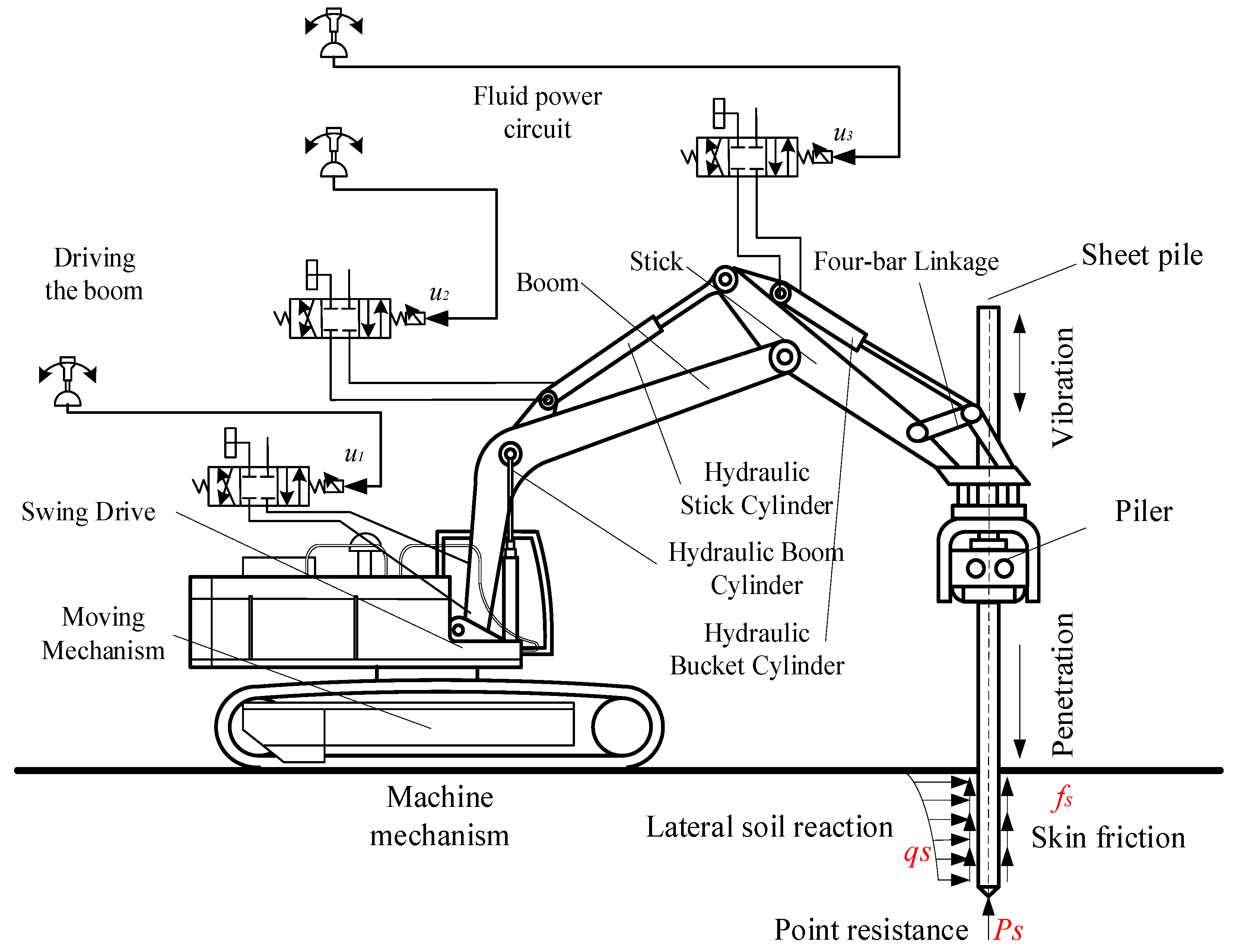
Currently, hydraulic pile drivers have emerged as the predominant choice in the pile driver market, owing to their robust power and efficient construction capabilities. The vibration pile driver excels in dual functionalities, seamlessly handling both pile sinking and pulling operations. Its construction principle revolves around harnessing the high-frequency vibration generated by the exciter to propel the adjacent soil into forced vibrations through the pile body. This induces alterations in the soil structure, subsequently diminishing the friction between the pile body and the surrounding soil. Consequently, the resistance encountered during both pile sinking and pulling operations is significantly minimized [37]. The work process consists of phases, where the excavator–piler combination unloads the piles from the truck and transports them to the workplace to drive them into the ground. After adjusting the drive line to the vertical, the vibratory unit works to compensate for the combined effects of point and skin friction of the soil, while the large translatory motion of the pile is fed by the excavator boom [3], as shown in Figure 1. The figure illustrates the schematic diagram of the side-grip hydraulic vibration pile driver mechanism. The operational components predominantly include the moving mechanism, swing drive, boom, stick, four-bar linkage, and swinging mechanism. These components are characterized by rotational joints, collectively constituting a six-degree-of-freedom (6-DOF) serial mechanism.

2.1. Swing Drive

The swing drive comprises a slewing motor, a set of interlocking large and small gears, and a slewing support platform. The complete robotic arm system is securely mounted on the swinging support platform. In operation, a gear pump channels high-pressure oil to propel the slewing motor, facilitating the meshing transmission of the large and small gears. This synchronized movement achieves the rotation of the swing support platform. Throughout the operational sequence, the mechanical arm system undergoes controlled rotation by manipulating the swing drive.

2.2. Boom, Stick and the Four-Bar Linkage

The boom, affixed to the slewing support platform, undergoes elevation and descent through the action of the boom cylinder, thereby influencing the entire robotic arm’s vertical movement. Extending forward and backward is accomplished by the bucket rod, securely attached at the boom’s end, and propelled by the bucket rod cylinder. Additionally, the four-bar linkage mechanism, connected to the extremity of the bucket rod, experiences movement through the four-bar linkage cylinder, facilitating the motion of the end deflection mechanism. The collaborative operation of the boom, bucket rod, four-bar linkage mechanism, and slewing device orchestrates the dynamic repositioning of the pile body within the defined working range.

2.3. Swinging Mechanism and Gripper

The deflection mechanism of the pile driver is illustrated in Figure 2, featuring the swinging mechanism comprised of essential components such as the swing cylinder, exciter, and gripper. The gripper, functioning as an end effector and a sub-mechanism of the swinging mechanism, is responsible for securely clamping objects. This swinging mechanism is intricately linked to the four-bar linkage, possessing two degrees of freedom.

The first degree of freedom involves a set of swing cylinders strategically positioned on the left and right sides. By manipulating these cylinders, precise control is exerted, allowing the clamped pile body to rotate left and right around the swinging joint. The second degree of freedom is realized through a rotary joint situated beneath the swinging joint. This rotary joint facilitates the rotation of the clamped pile body around its axis, contributing to the mechanism’s overall flexibility and adaptability during operation.

3. Kinematic Description of Working Mechanism System

3.1. Establishment of the Coordinate System

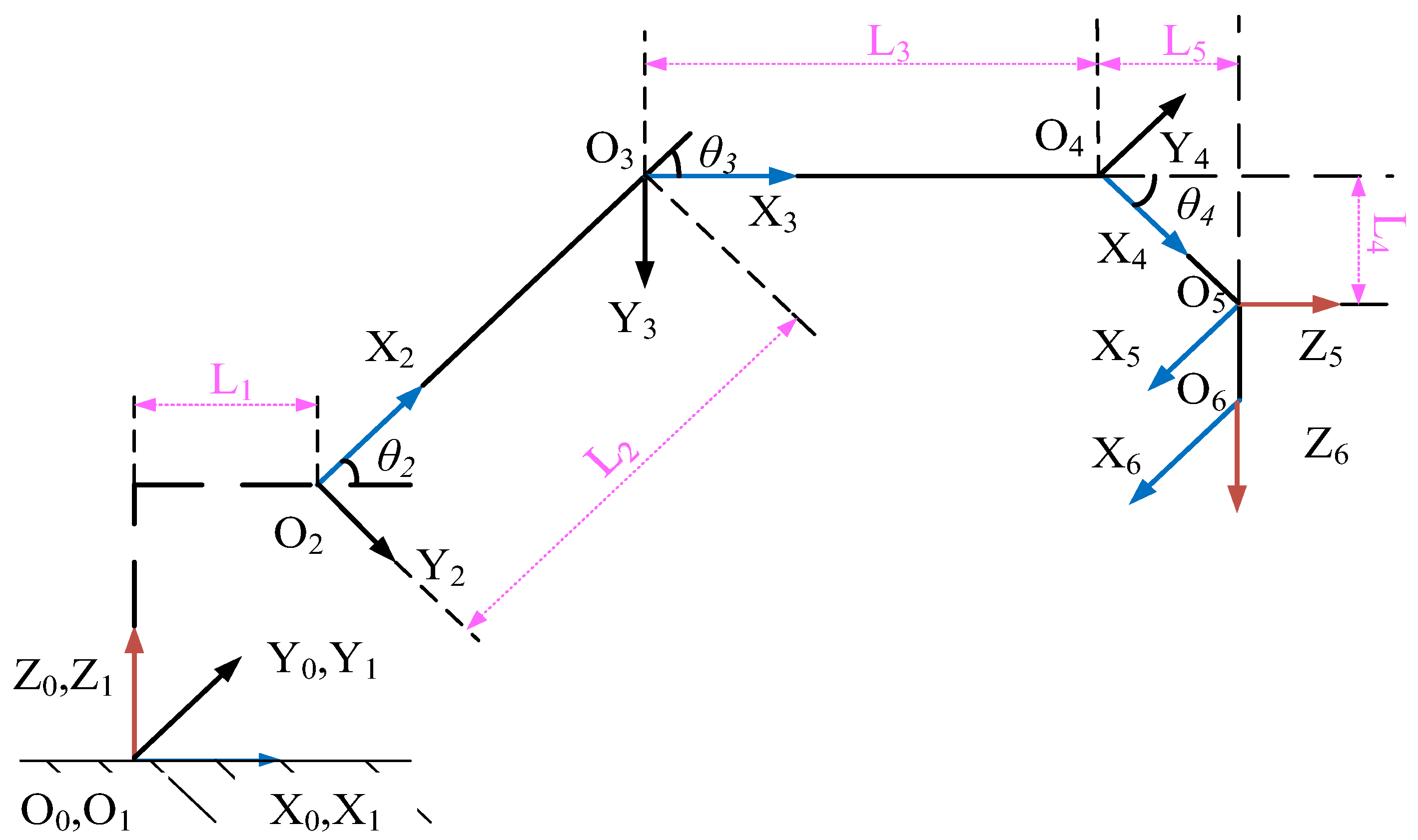
The side-clamp pile driver is a sequential robotic arm with six joints, involving rotating or moving elements and connecting rods. These connecting rods are linked to the base of the robotic arm. The structure of the robotic arm follows the D-H coordinate system, with an improved version based on its configuration [38]. The base coordinate system denoted as X₀Y₀Z₀, aligns with the coordinate system X₁Y₁Z₁ at the turning device. Sequentially, coordinate systems are established at each joint. The coordinate system X₆Y₆Z₆ is defined as the gripper coordinate system at the end-clamping mechanism of the pile driver. In the D-H coordinate system, each connecting rod comprises four independent parameters. These parameters are defined as follows: link a_i−1 = distance from z_i−1 to z_i along x_i−1, rotation α_i−1 = rotating from z_i to z_i−1 around x_i−1, distance d_i = distance from x_i−1 to x_i along z_i, joint rotation θ_i = rotating from x_i−1 to x_i around z_i. The D-H parameters of the robotic arm can be determined based on the coordinate system established in Figure 3 and the dimensions of the robotic arm link, as listed in

Table 1. Parameters of the side-clamp pile driver D-H.

Link	ai−1	αi−1 (rad)	di	θi	Range θi (rad)
1	0	0	0	θ1	(−π,π)
2	L1	π/2	0	θ2	(0,π/3)
3	L2	0	0	θ3	(−π/3,0)
4	L3	0	0	θ4	(−π/3,0)
5	L4	−π/2	L5	θ5	(−π/6,π/6)
6	0	−π/2	0	θ6	(−π,π)

.

3.2. Forward Kinematics Analysis

Forward kinematics is to solve the pose of the end effector of the robot arm relative to the robot base coordinate system by knowing the joint angle of each link and the structural size of the link. According to the homogeneous coordinate transformation method, the general expression of the transformation matrix between two adjacent joint coordinate systems is as follows:

$$\begin{array}{l}{}_i{}^{i-1}T=Rot(x,{\alpha }_{i-1})Trans(x,a_{i-1})Trans(z,d_i)Rot(z,{\theta }_i)\\ =\left[\begin{array}{cccc}\cos ({\theta }_i)& -\sin ({\theta }_i)& 0& a_{i-1}\\ \sin ({\theta }_i)\cos ({\alpha }_{i-1})& \cos ({\theta }_i)\cos ({\alpha }_{i-1})& -\sin ({\alpha }_{i-1})& -d_i\sin ({\alpha }_{i-1})\\ \sin ({\theta }_i)\sin ({\alpha }_{i-1})& \cos ({\theta }_i)\sin ({\alpha }_{i-1})& \cos ({\alpha }_{i-1})& d_i\cos ({\alpha }_{i-1})\\ 0& 0& 0& 1\end{array}\right]\end{array}$$

(1)

Putting the connecting rod parameters in Table 1 into Formula (1), and multiplying the transformation matrices in sequence, the transformation matrix of the robot arm end coordinate system {6} under the base coordinate system {0} can be obtained as follows:

$${}_6{}^{0}T={}_1{}^{0}T\cdot {}_2{}^{1}T\cdot {}_3{}^{2}T\cdot {}_4{}^{3}T\cdot {}_5{}^{4}T\cdot {}_6{}^{5}T=\left[\begin{array}{cccc}{n}_x& o_x& a_x& p_x\\ n_y& o_y& a_y& p_y\\ n_z& o_z& a_z& p_z\\ 0& 0& 0& 1\end{array}\right]$$

(2)

The values of each element of Formula (2) are obtained as follows:

$$\begin{array}{l}{n}_x=c_6\left(s_1{c}_5+s_5{c}_1{s}_{234}\right)-s_6{c}_1{c}_{234}\hfill \\ n_y=-s_6{s}_1{c}_{234}-c_6\left(c_1{c}_5-s_5{s}_1{s}_{234}\right)\hfill \\ n_z=-s_6{s}_{234}-c_6{s}_5{c}_{234}\hfill \\ o_x=-s_6\left(s_5{s}_1+s_5{c}_1{s}_{234}\right)-c_6{c}_1{c}_{234}\hfill \\ o_y=s_6\left(c_1{c}_5-s_5{s}_1{s}_{234}\right)-c_6{s}_1{c}_{234}\hfill \\ o_z=s_5{s}_6{c}_{234}-c_6{s}_{234},a_x=c_5{c}_1{s}_{234}-s_1{s}_5\hfill \\ a_y=c_5{s}_1{s}_{234}+c_1{s}_5,a_z=-c_5{c}_{234}\hfill \\ p_x=L_1{c}_1+L_3{c}_1{c}_{23}+L_4{c}_1{s}_{234}+L_5{c}_1{c}_{234}+L_2{c}_1{c}_2\hfill \\ p_y=L_1{s}_1+L_3{s}_1{c}_{23}+L_2{c}_2{s}_1+L_4{s}_1{s}_{234}+L_5{s}_1{c}_{234}\hfill \\ p_z=L_2{s}_2+L_3{s}_{23}-L_4{c}_{234}+L_5{s}_{234}\hfill \end{array}$$

and c_i = cos(θ_i), s_i = sin(θ_i).

3.3. Inverse Kinematics Model Analysis

To manipulate the orientation of the pile body, solving the inverse kinematics of the robotic arm becomes imperative. In simpler terms, this entails determining the angles of each joint in the robotic arm when provided with the desired orientation of the end effector coordinate system concerning the base coordinate system.

The mechanical arm characteristics of the side-clamp pile driver under investigation adhere to the Pieper criterion, implying the presence of an analytical solution. The proposed solution method involves employing the inverse matrix transformation method. The procedural steps are outlined below.

Given that the end effector pose is ${}_6{}^{0}T$, the transformation matrix of the end coordinate system in the base coordinate system can be obtained as follows:

$$\begin{array}{l}{}_6{}^{1}T={}_1{}^{0}T^{-1}\cdot {}_6{}^{0}T=\left[\begin{array}{cccc}{c}_1& s_1& 0& 0\\ -s_1& c_1& 0& 0\\ 0& 0& 1& 0\\ 0& 0& 0& 1\end{array}\right]\left[\begin{array}{cccc}{n}_x& o_x& a_x& p_x\\ n_y& o_y& a_y& p_y\\ n_z& o_z& a_z& p_z\\ 0& 0& 0& 1\end{array}\right]\\ =\left[\begin{array}{cccc}{c}_1{n}_x+n_y{s}_1& c_1{o}_x+o_y{s}_1& a_x{c}_1+a_y{s}_1& c_1{p}_x+p_y{s}_1\\ c_1{n}_y-n_x{s}_1& c_1{o}_y-o_x{s}_1& a_y{c}_1-a_x{s}_1& c_1{p}_y-p_x{s}_1\\ n_z& o_z& a_z& p_z\\ 0& 0& 0& 1\end{array}\right]\end{array}$$

(3)

where

$${}_6{}^{1}T={}_2{}^{1}T\cdot {}_3{}^{2}T\cdot {}_4{}^{3}T\cdot {}_5{}^{4}T\cdot {}_6{}^{5}T$$

(4)

Let the (2, 4) elements in the matrices of Formulas (3) and (4) be equal, and we can obtain the following:

$${\theta }_1=\arctan (\frac{p_y}{p_x})$$

(5)

Let the elements on both sides of the matrices (1, 4) and (3, 4) of Formulas (3) and (4) be equal, and we can obtain the following:

$${\theta }_3=\arctan (\frac{s_3}{c_3})$$

(6)

Among them, we can obtain the following:

$$\begin{array}{l}{m}_1={(c_1{p}_x+s_1{p}_y-L_5{c}_{234}-L_1-L_4{s}_{234})}^2\\ m_2={(p_z+L_4{c}_{234}-L_5{s}_{234})}^2-L_2^2-L_3^2\\ c_3=\frac{(m_1+m_2)}{2}\times L_2\times L_3\\ s_3=\pm \sqrt{1-c_3^2}\end{array}$$

(7)

After sorting out Formulas (3) and (4), we can obtain the following:

$${}_6{}^{4}T={}_4{}^{3}T^{-1}\cdot {}_3{}^{2}T^{-1}\cdot {}_2{}^{1}T^{-1}\cdot {}_1{}^{0}T^{-1}\cdot {}_6{}^{0}T={}_5{}^{4}T\cdot {}_6{}^{5}T$$

(8)

Let the elements (2, 3) on both sides of the matrix of Formula (8) be equal, and we can obtain θ₂₃₄ as follows:

$${\theta }_{234}=\arctan (\frac{s_{234}}{c_{234}})$$

(9)

Here,

$$\begin{array}{l}{s}_{234}=(p_y^2-p_x^2)a_x-2a_y{p}_x{p}_y\\ c_{234}=(p_y^2+p_x^2)a_z\end{array}$$

(10)

Let the elements of matrices (1, 3) and (3, 3) of Formula (8) be equal and we can obtain the following:

$${\theta }_5=\arctan (\frac{s_5}{c_5})$$

(11)

Here,

$$\begin{array}{l}{s}_5=c_1\left(a_y{c}_1-a_x{s}_1\right)-s_1\left(a_x{c}_1+a_y{s}_1\right)\\ c_5=s_{234}\left(\left(c_{1 }^2-s_{1 }^2\right)a_x+2s_1{c}_1{a}_y\right)-a_z{c}_{234}\end{array}$$

(12)

Let the elements on both sides of Formulas (3) and (4) matrices (1, 4) (3, 4) be equal to obtain the following:

$${\theta }_2=\arctan (\frac{s_2}{c_2})$$

(13)

Here,

$$\begin{array}{l}{c}_2=\frac{k_2{L}_3{s}_3+k_1(L_2+L_3{c}_3)}{{(L_2+L_3{c}_3)}^2+{(L_3{s}_3)}^2}\\ s_2=\frac{k_2{L}_3{s}_3(L_2+L_3{c}_3)+k_1(L_2+L_3{c}_3){)}^2}{({(L_2+L_3{c}_3)}^2+{(L_3{s}_3)}^2)L_3{s}_3}-\frac{k_1}{L_3{s}_3}\\ \begin{array}{l}{k}_1=c_1{p}_x+p_y{s}_1-L_5{c}_{234}-L_1-L_4{s}_{234}\hfill \\ k_2=p_z+L_4{c}_{234}-L_5{s}_{234}\hfill \end{array}\end{array}$$

(14)

Let the elements (2, 1) and (2, 2) on both sides of Formula (8) be equal, and we can obtain the following:

$${\theta }_6=\arctan (\frac{s_6}{c_6})$$

(15)

Here,

$$\begin{array}{l}{s}_6=n_z{s}_{234}+c_{234}(n_x(c_1^2-s_1^2)+2c_1{s}_1{n}_y)\\ c_6=o_z{s}_{234}+c_{234}(o_x(c_1^2-s_1^2)+2c_1{s}_1{o}_y)\end{array}$$

(16)

According to the above formula, the values of θ₃, θ₂₃₄, and θ₂ can be obtained as follows:

$${\theta }_4={\theta }_{234}-{\theta }_2-{\theta }_3$$

(17)

3.4. Relationship between Pile Body Posture and Hydraulic Cylinder Stroke

The pile body posture adjustment is finally completed through the joint adjustment of the hydraulic boom cylinder, hydraulic stick cylinder, four-bar linkage drive cylinder, and swinging mechanism. To realize the adjustment of the clamped object according to the desired posture, the joint angle θ_i must first be solved through the inverse kinematics of the manipulator, and then the mapping relationship between the joint rotation angle θ_i and the joint cylinder stroke λ_i must be established. Finally, the pile position can be achieved by controlling the cylinder stroke and posture adjustment. In this article, the corresponding relationship between the joint angles of the pile driver’s mechanical arm and its cylinder length is described below.

3.4.1. The Relationship between the Boom Joint Angle and Its Cylinder Length

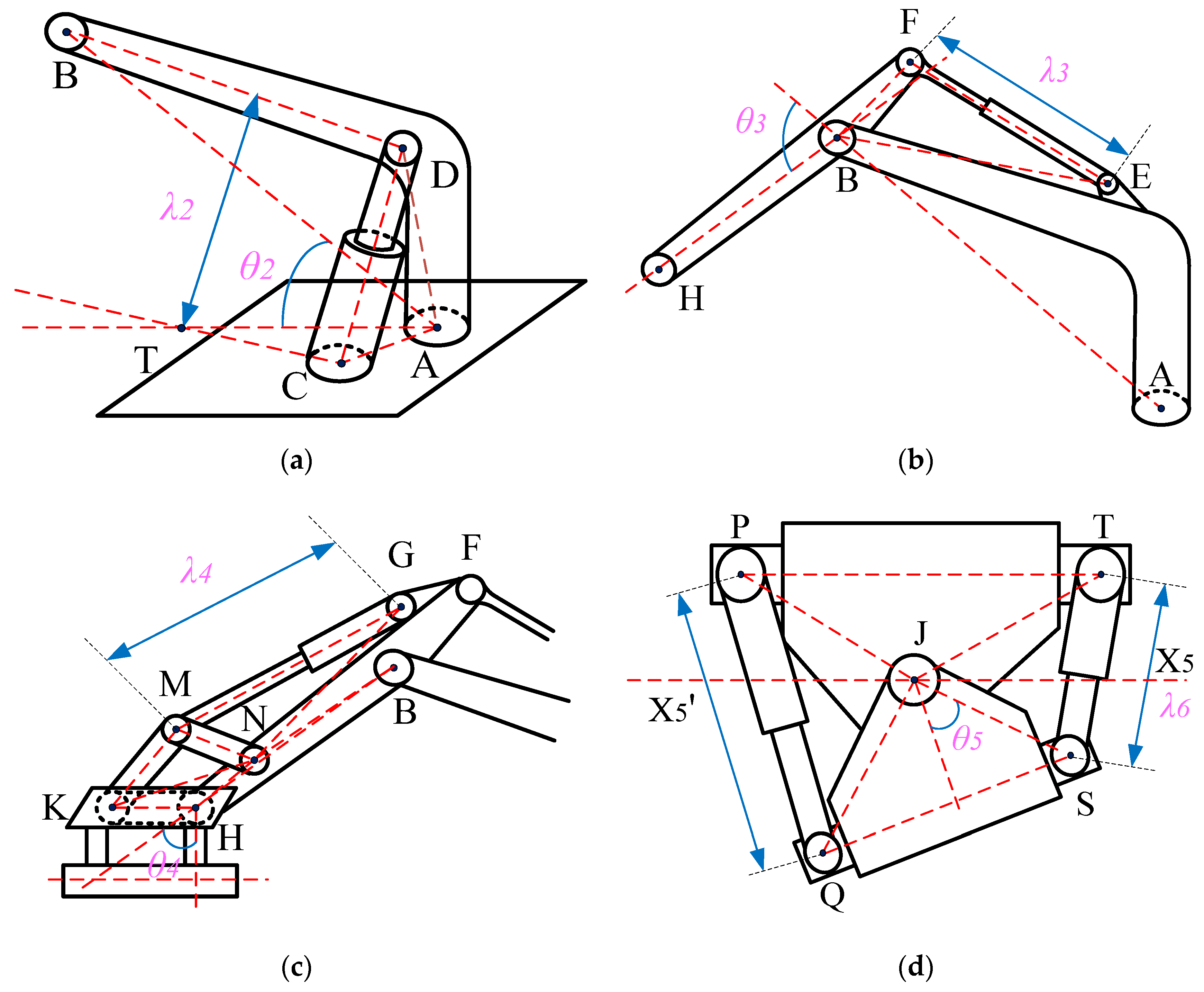
The schematic diagram of the vibration pile driver arm mechanism is shown in Figure 4a. In the figure, L_DC is the telescopic length of the boom cylinder to be found. In the triangle CAD it is obtained as follows:

$${\lambda }_2=L_{DC}=\sqrt{{L_{AC}}^2+{L_{AD}}^2-2\cdot L_{AC}\cdot L_{AD}\cdot \cos (\angle CAD)}$$

(18)

Here,

$$\angle CAD=\angle CAT+{\theta }_2+\angle BAD$$

3.4.2. The Relationship between Stick Joint Angle and Cylinder Length

The schematic diagram of the arm mechanism of the vibration pile driver is shown in Figure 4b. In the figure, L_EF is the length of the arm cylinder to be found. According to the triangle EBF, it can be obtained as follows:

$${\lambda }_3=L_{EF}=\sqrt{{L_{BE}}^2+{L_{BF}}^2-2\cdot L_{BE}\cdot L_{BF}\cdot \cos (\angle EBF)}$$

(19)

Here,

$$\angle EBF={180}^{\circ }+{\theta }_3-\angle FBH-\angle ABE$$

3.4.3. The Relationship between the Four-Link Joint Angle and Its Cylinder Length

The schematic diagram of the four-bar linkage mechanism of the pile driver is shown in Figure 4c.

As can be seen from Figure 4c, in the triangle MNG,

$${\lambda }_4=L_{MG}=\sqrt{{L_{MN}}^2+{L_{NG}}^2-2\cdot L_{MN}\cdot L_{NG}\cdot \cos (\angle MNG)}$$

(20)

Taking joint point H as the center of the circle, we can obtain the following:

$$L_{KN}=\sqrt{{L_{KH}}^2+{L_{HN}}^2-2L_{KH}\cdot L_{HN}\cdot \cos (\angle KHN)}$$

(21)

Taking joint point N as the center of the circle, we can obtain the following:

$$\angle KNH=\arccos (\frac{{L_{HN}}^2+{L_{KN}}^2-{L_{KH}}^2}{2\cdot L_{HN}\cdot L_{KN}})$$

(22)

$$\angle KNM=\arccos (\frac{{L_{MN}}^2+{L_{KN}}^2-{L_{KM}}^2}{2\cdot L_{MN}\cdot L_{KN}})$$

(23)

Therefore, we can obtain the following:

$$\angle MNG={360}^{\circ }-\angle GNB-\angle BNH-\angle HNK-\angle KNM$$

3.4.4. The Relationship between the Swinging Joint Angle and the Length of the Swinging Cylinder

The joint angle of the swinging mechanism and the geometric structure of the drive cylinder of the swinging mechanism are shown in Figure 4d. P, Q, T, and S are the installation positions of the swinging cylinder, and point J is the joint point of the swinging mechanism. The lengths of L_PT, L_PJ, L_TJ, L_QJ, L_QS, and L_SJ in the figure are all fixed values. According to triangles PJQ and SJT, we can know the following:

$${\lambda }_5=L_{PQ}=\sqrt{{L_{PJ}}^2+{L_{QJ}}^2-2\cdot L_{PJ}\cdot L_{QJ}\cdot \cos (\angle PJQ)}$$

(24)

$${\lambda }_6=L_{TS}=\sqrt{{L_{TJ}}^2+{L_{SJ}}^2-2\cdot L_{TJ}\cdot L_{SJ}\cdot \cos (\angle SJT)}$$

(25)

Here,

$$\angle PJQ={180}^{\circ }-{\theta }_5-\frac{\angle QJS}{2}+\angle X_5^{\prime }JP$$

$$\angle SJT={\theta }_5-\frac{\angle X_{4}JS}{2}+\angle X_{5}JP$$

3.5. Forward Kinematics Simulation

To verify the correctness of the kinematics model of the pile driver’s manipulator, MATLAB’s robotics toolbox was used to perform kinematic modeling and simulation. First, the MATLAB environment was used to import the D-H parameters in Table 1 through the Link function, and the Serial Link function was used to build the robotic arm model. Then, given a set of initial joint angles q₁ = [0,0,0,0,0,0], at this time, the pile driver mechanical arms are in a horizontal state relative to the zero point posture. If the pile driver is in working condition to keep the pile body sinking vertically, the boom, stick, and yaw joint angles will change. Within the working range, q₂ = [−60, 30, −20, −10, 0, 0]. The length of each connecting rod of the pile driver is L₁ = 20 cm, L₂ = 80 cm, L₃ = 60 cm, L₄ = 30 cm, and L₅ = 10 cm. Bringing the vectors q₁ and q₂ into the kinematics forward solution model solved above, the pose matrix of the end effector is obtained as follows:

$${}_6{}^{0}T^1=\left[\begin{array}{cccc}\begin{array}{c}0\\ -1\\ 0\\ 0\end{array}& \begin{array}{c}-1\\ 0\\ 0\\ 0\end{array}& \begin{array}{c}0\\ 0\\ -1\\ 0\end{array}& \begin{array}{c}190\\ 0\\ -30\\ 1\end{array}\end{array}\right],\hspace{1em}\hspace{1em}\hspace{1em}{}_6{}^{0}T^2=\left[\begin{array}{cccc}\begin{array}{c}-0.866\\ -0.5\\ 0\\ 0\end{array}& \begin{array}{c}-0.5\\ 0.866\\ 0\\ 0\end{array}& \begin{array}{c}0\\ 0\\ -1\\ 0\end{array}& \begin{array}{c}89.19\\ -154.5\\ -20.42\\ 1\end{array}\end{array}\right]$$

The result of the kinematics forward solution model is ${}_6{}^{0}T^1$, ${}_6{}^{0}T^2$ matrices which are exactly the same as the matrices solved by the Fkine function in the MATLAB robotics toolbox, which verifies the correctness of the forward solution model. The simulation model of its robotic arm is shown in Figure 5.

3.6. Inverse Kinematics Simulation

Inverse kinematics simulation gives the pose matrix of the actuator coordinates at the end of the robot arm, uses the matrix as a known quantity to calculate the angles corresponding to each joint of the robot arm, and inputs this angle as the forward kinematics solution and brings it into the robot tool. If the solved matrix is consistent with the given pose matrix, the correctness of the inverse kinematic solution model is verified.

Randomly select a set of joint angles S₁ = [50, 30, −20, −10, 5, 20] within the working range of the pile driver, and use the Fkine function of the robot toolbox to solve the corresponding matrix:

$${}_6{}^{0}T^3=\left[\begin{array}{cccc}\begin{array}{c}0.4973\\ -0.8637\\ -0.0819\\ 0\end{array}& \begin{array}{c}-0.865\\ -0.5\\ 0.0298\\ 0\end{array}& \begin{array}{c}-0.0667\\ 0.056\\ -0.99\\ 0\end{array}& \begin{array}{c}114.7\\ 136.6\\ 40.42\\ 1\end{array}\end{array}\right]$$

A 6-DOF manipulator may have eight sets of joint angle combinations in the same posture. However, in the actual operation of the pile driver manipulator, there will only be one set of solutions due to the stroke limitations of each joint mechanism and the drive cylinder. Bring the matrix ${}_6{}^{0}T^3$ as the input value into the kinematics inverse solution model, and solve a set of solutions S₂ = [50.007, 30.002, −20.001, −10.0, 5.00, 20.001]. Bring the solved joint angle S₂ into the kinematics forward solution model, and compare the solved matrix ${}_6{}^{0}T^4$ with the original ${}_6{}^{0}T^3$ matrix.

$${}_6{}^{0}T^4=\left[\begin{array}{cccc}\begin{array}{c}0.4973\\ -0.8637\\ -0.0819\\ 0\end{array}& \begin{array}{c}-0.865\\ -0.5\\ 0.0298\\ 0\end{array}& \begin{array}{c}-0.0667\\ 0.056\\ -0.99\\ 0\end{array}& \begin{array}{c}114.7\\ 136.6\\ 40.42\\ 1\end{array}\end{array}\right]$$

The results are the same, which verifies the correctness of the inverse solution model.

3.7. Workspace Analysis

The working space of the pile driver’s robotic arm is a collection of points that the end effector can reach in the space. The working space reflects the structural characteristics of the robotic arm. Analysis of its characteristics is of great significance for optimizing the structural research of the robotic arm and the performance of the robotic arm.

This article uses the Monte Carlo method [14,15,16] to conduct workspace simulation analysis. The values of the six joint variables are randomly selected within the value range of the six joint variables. The position of the end actuator constitutes a set of points that constitutes the robot arm workspace. In this paper, N = 30,000 random values are selected for each joint variable, and a forward kinematics solution is performed on N groups of joint vectors to obtain the position set of the end actuator in space. The results are shown in Figure 6a. To clearly and intuitively observe the simulation represented, the graphics are projected on the XOY, XOZ, and YOZ planes, and the results are shown in Figure 6b–d. From the working space point cloud diagram in Figure 6a, it can be seen that the working space of the pile driver is approximately a sphere, with a large working range and a uniform distribution of points in the working space, indicating that the mechanical arm structure is reasonably arranged. According to Figure 6b, the range of X is between −1800~−900 mm and 900~1800 mm and the range of Y is between −1800~−900 mm and 900~1800 mm. As shown in Figure 6c,d, the range of Z is from −1000 to 1500 mm.

4. Trajectory Planning

Piling machines often operate unmanned in hazardous environments, like geological disaster areas, repairing damaged infrastructure. Unmanned pile drivers are used for underwater bridge maintenance and repair, stabilizing piers. In offshore platform construction, they drive pile foundations to ensure stability, particularly in deep-sea areas, reducing risks to personnel from underwater environments and high-pressure gases. The system must execute tasks remotely or through preset programs. In dynamic pile driving operations, studying obstacle avoidance motion planning strategies is crucial. Traditional robotic arm methods rely heavily on manual programming, resulting in inefficiency and adaptability issues for obstacle avoidance. To address this, robotic arms need autonomous obstacle-free trajectory planning, involving processing information from the starting point to the target, exploring collision-free joint angle configurations, and completing pile driving tasks. Advanced path-planning algorithms are essential for efficient, safe, and compliant robotic arm operations.

4.1. Gray Wolf Algorithm

The SI algorithm often finds inspiration from the collective behavior observed in various animal species [39], which typically simulates the hunting process of prey, searching for food based on local interactions between group members or based on the environment (granular) [40]. Therefore, grouped groups are self-organizing. It is typically initiated by a set of candidate solutions. Usually, groups can be divided into two main groups, leaders and followers, where interaction occurs by attracting followers to the leader. Therefore, convergence towards the optimal solution can take place. GWO is the fastest growing SI algorithm introduced by Mirjalili et al. [41] to mimic the hunting behavior of gray packets in nature. GWO is a powerful optimizer because it has impressive features compared to other models, such as easy adaptation, no parameters, no derivatives, no memory, no computation, flexibility, and complete sound. In the initial search phase, GWO starts with high intensity in the exploration phase, and in the final run, GWO gradually shifts its focus to the development phase through the positions of the three best leaders. The social division of labor among wolves includes alpha wolf, beta wolf, delta wolf, and omega wolf.

The hunting model of wolf packs is showed in Figure 7. During the iteration process, the objective function value of the optimal wolf after each iteration is compared with the value of the alpha wolf in the previous generation. If it is better, the position of the alpha wolf is updated. If there are multiple horses at this time, randomly select one to become the alpha wolf. The alpha wolf does not perform three intelligent behaviors and directly enters the next iteration until it is replaced by other stronger omega wolves. The behaviors are described below.

• Wandering behavior: In the solution space, the best S omega wolves other than the alpha wolf are considered beta wolves, and the fitness of the prey searched by each beta wolf is calculated separately. If it is greater than the fitness of the alpha wolf, the beta wolf becomes the alpha wolf and initiates a new summoning behavior. Otherwise, the beta wolf will choose the direction with the strongest odor and the odor concentration Y_i greater than the current position in the direction p and move forward one step as follows:

$$x_{id}^p=x_{id}+\sin (2\pi \times \frac{p}{h})\times ste{p}_s^d$$

(26)

where $ste{p}_s^d$ is the walking step length, h is the walking direction, p = 1, 2,…. Repeat the above wandering behavior until there is a scent concentration Y_i > Y_lead of a certain beta wolf, then beta wolf i replaces the alpha wolf and initiates a summoning behavior, or reaches the maximum number of wandering times T_max.

• Summoning behavior: After the wandering behavior ends, an alpha wolf will be generated. The alpha wolf uses a howling method to initiate a summoning behavior, quickly summoning the surrounding M delta wolves towards their position. The delta wolves quickly approach the alpha wolf with a running stride and search for prey. During the delta wolf attack, if the prey has a higher adaptability, let the delta wolf replace the alpha wolf. When the distance between the delta wolf and the alpha wolf is less than the threshold, it switches to besieging behavior. When the delta wolf j undergoes the k + 1 iteration, its position in the d-dimensional space can be expressed as follows:

$$x_{jd}^{k+1}=x_{jd}^k+ste{p}_b^d\times \frac{g_d^k-x_{jd}^k}{\left|g_d^k-x_{jd}^k\right|}$$

(27)

where $g_d^k$ is the position of the alpha wolf of the k generation group in the d-dimensional space, $x_{jd}^k$ is the current position of the delta wolf j, and $ste{p}_b^d\times \frac{g_d^k-x_{jd}^k}{\left|g_d^k-x_{jd}^k\right|}$ is the gradual gathering of the delta wolf j towards the position of the alpha wolf. On the way, if the odor concentration of the delta wolf is Y > Y_lead, then the delta wolf i replaces the alpha wolf and initiates a summoning behavior. If Y < Y_lead, the delta wolf continues to attack until d_is ≤ d_near, joining the attack on the prey, that is, entering a siege behavior as follows:

$$d_{near}=\frac{1}{D\omega }{\displaystyle \sum _{d=1}^D\left|{\max }_d-{\min }_d\right|}$$

(28)

where ω is for the distance determination factor, and the range of values for the d-dimensional variable to be optimized is [min_d, max_d].

• Siege behavior: A combination of delta wolves and beta wolves to encircle and capture prey. The delta wolf sensed the call of the alpha wolf and immediately ran towards the position of the alpha wolf. During the running process, if it found that the prey had higher adaptability, it immediately replaced the original alpha wolf and commanded other wolves to take action.

$$x_{id}^{k+1}=x_{id}^k+\lambda \times ste{p}_w^d\times \left|G_d^k-x_{id}^k\right|$$

(29)

here λ is a random number within the interval of [−1,1], uniformly distributed, $ste{p}_w^d$ is the attack step size of omega wolf i (including beta and delta wolves) when engaging in besieging behavior in the d-dimension space. After adopting a siege behavior, if the odor concentration perceived by omega wolf i is greater than the concentration perceived at its original position, the position of omega wolf i will be updated; otherwise, the position of omega wolf i will remain unchanged. The relationship between the walking stride $ste{p}_s^d$, attacking stride $ste{p}_b^d$, and siege stride $ste{p}_w^d$ of omega wolves is as follows:

$$ste{p}_s^d=\frac{ste{p}_b^d}{2}=2\times ste{p}_w^d\times \frac{\left|M_d-m_d\right|}{C}$$

(30)

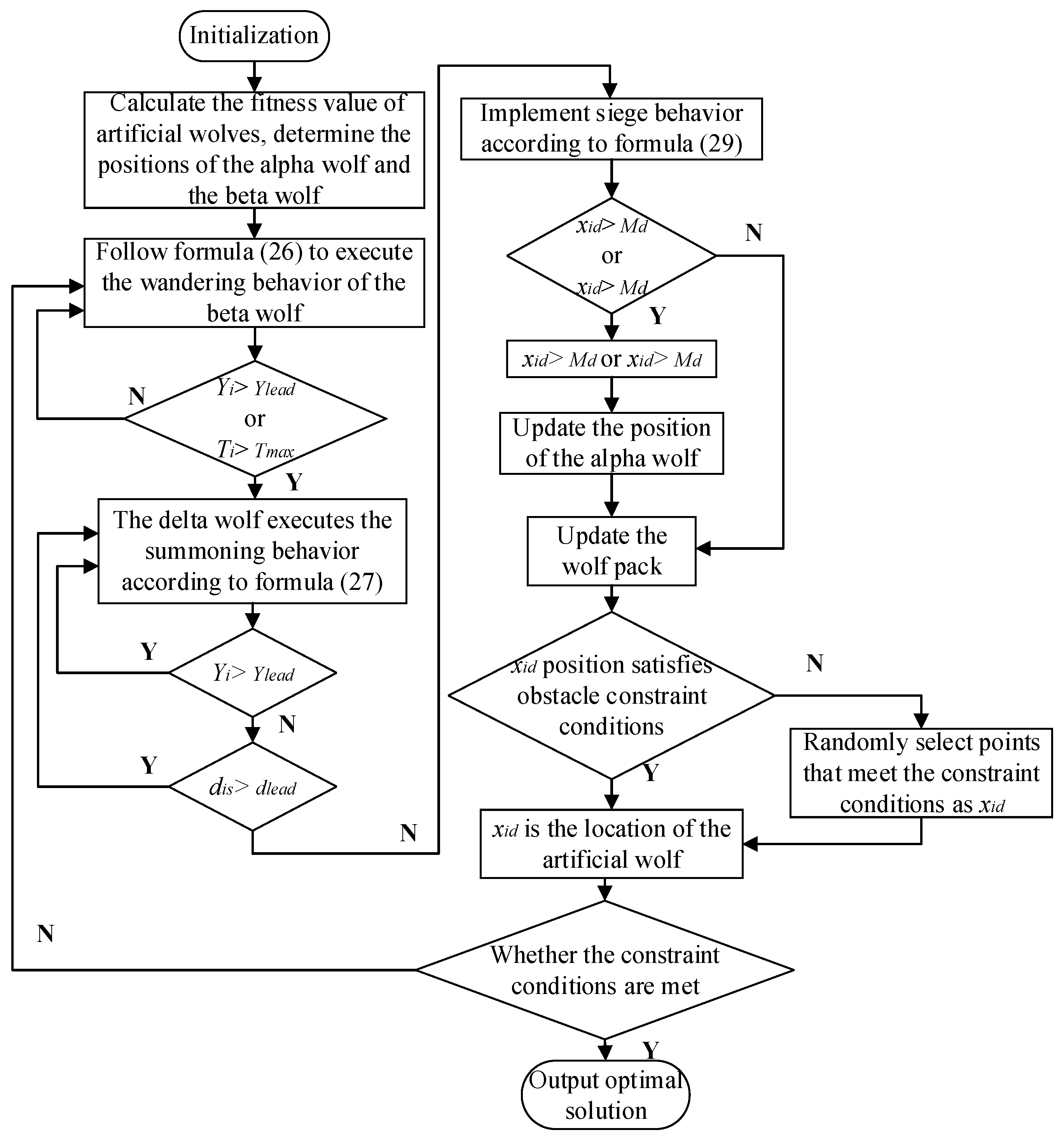
The path planning process diagram based on GWO is shown in Figure 8.

4.2. Improved GWO

4.2.1. Adaptive Wandering and Sieging Strategy

In the basic GWO algorithm, the update step size of the wandering and sieging behavior positions of each generation of wolf packs is fixed and invariant, and both are related to the walking step size. This fixed step size approach can cause a slow convergence speed in the initial stage of the algorithm and a decrease in search precision in the later stage, leading to the algorithm falling into the local optima. Therefore, this article adopts an adaptive step size approach to optimize the walking step size and running step size in the basic Gray Wolf Algorithm, and improves the search accuracy and convergence speed of the algorithm by reasonably changing the adaptive step size.

The article adopts an adaptive step size of

$$step=rand\times {‖x_i-X_{lead}‖}_2$$

where rand represents a random number between [0, 1]; x_i represents the current position of the wolf i; X_lead represents the position of the alpha wolf.

4.2.2. Adaptive Walk Behavior Based on Levy Flight Strategy

Levy flight is a random search method that follows the Levy distribution and has good search randomness and global optimization ability. Using the Levy flight search strategy for a global random search can make the distribution of wolf scouts more extensive in the search space, improve the algorithm’s global search ability, and easily jump out of local optimal solutions.

The formula for updating the position of Levy flight is as follows:

$$x_i^{t+1}=x_i^t+l\oplus Levy\left(\lambda \right)$$

where l represents step weight, and $l=0.01\times \left(x_i^t-x_{ibest}\right)$, $\oplus$ represents point-to-point multiplication; Levy represents a random path that follows the Levy distribution, satisfying the following conditions:

$$Levy~u=t^{-\lambda },1<\lambda \le 3$$

The formula for updating the position of the adaptive walking behavior of the beta wolf with the addition of Levy flight strategy is as follows:

$$x_{id}^t=x_{id}+\sin \left(2\pi \times \frac{p}{h}\right)\times rand\times {‖x_i-X_{lead}‖}_2+l\oplus Levy\left(\lambda \right)$$

where $x_{id}^t$ is the position of the beta wolf i in the d-dimensional space in the t iteration, and X_lead is the position of the alpha wolf (i.e., prey).

Based on the above formula for updating the position of the wandering behavior, the algorithm has the excellent global search ability of Levy flight, while dynamically adjusting the forward step size of the beta wolf to compensate for the slow convergence speed of Levy flight strategy.

4.2.3. Adaptive Summoning Behavior

During the summoning behavior, delta wolves rush toward the position of their prey (i.e., the position of the alpha wolf). If the target fitness value Y_j perceived by the delta wolf during the attack is smaller than the target fitness value Y_lead perceived by the alpha wolf, then Y_lead = Y_j, and the delta wolf replaces the alpha wolf to initiate the summoning behavior again. If the target fitness value Y_j perceived by the delta wolf is greater than the target function value Y_lead perceived by the alpha wolf, the delta wolf will continue to perform the rushing behavior until the distance between the delta wolf and the alpha wolf is less than d_near.

The formula for updating the position of delta wolf j in the t + 1 iteration is as follows:

$$x_{jd}^{t+1}=x_{jd}^t+rand\times {‖x_{jd}^t-x_{lead}^t‖}_2\times \frac{x_{lead}^t-x_{jd}^t}{\left|x_{lead}^t-x_{jd}^t\right|}$$

where $x_{jd}^t$ is the position of the delta wolf j in the d-dimensional space in the t iteration.

4.3. Simulation Environment and Experimental Data Preparation

In order to verify the effectiveness of the multi-strategy improved GWO algorithm in 3D path planning of robotic arms, the basic GWO algorithm and the proposed multi-strategy improved GWO algorithm were used for 3D path planning simulation under the same conditions. The simulation experimental environment is a computer with a Win10 64-bit operating system, featuring an AMD Ryzen 7 3750H 2.30 GHz processor, and 8 GB memory configuration, manufactured by AMD and assembled by Asus in China. The simulation experiment software used is MATLAB R2021b. At the same time, in order to further demonstrate the effectiveness and superiority of the improved GWO algorithm, this paper added comparative experiments of the improved GWO algorithm, basic GWO algorithm, basic ACA, basic GA, and basic AFSA in the 3D environment simulation experiment.

The task space for simulating the environment and preparing experimental data for path planning is 100 mm × 100 mm × Within 100 mm; five obstacles are set up in the space, all of which are spherical. The relevant parameter settings are as follows: the starting point coordinate is Start = [1, 1, 1], and the target point coordinate is Goal = [100, 100, 100]. The GWO parameters are shown in

Table 2. Parameter settings for Gray Wolf Algorithm.

Parameter	Meaning	Value
N	Number of wolf packs	100
α	Scale Factor of Beta Wolves	0.5
S	Step factor	100
Kmax	Maximum number of walks	10
ω	Distance determination factor	3
β	Wolf pack update ratio factor	3
h	Number of walking directions	20
Tmax	Maximum number of iterations	50
PC	Selection probability	0.6

.

The parameter settings for basic AFSA are as follows: number of fish schools is 50, perceived distance of artificial fish is 50, the maximum step size of artificial fish movement is 3, crowding factor is 10, the maximum number of iterations for a single fish is 50, iterations is 100, and dimension of solution is 3. The parameter settings for basic GA are as follows: population size is 5, chromosome length is 5, cross probability is 0.8, selection probability is 0.5, and mutation probability is 0.2. The parameter settings for basic ACA are as follows: ant number is 100, pheromone importance factor is 10, heuristic function importance factor is 1; pheromone volatilization factor is 0.1, constant is 1, maximum number of iterations is 100, and number of sliced structures is 9.

4.4. Simulation Results and Analysis

Figure 9 shows the convergence curve of the GWO for the entire path planning. It should be noted that the optimization problem studied in this article is a minimization problem, that is, the smaller the fitness value, the better the solution. From Figure 9, it can be seen that the GWO converges quickly to a very small fitness value. At around 20 iterations, the GWO falls into the local optima; however, as the number of iterations increases, the optimizer breaks through local optimal stagnation and continues to converge towards reducing the fitness value. The random dispersion strategy in GWO can effectively overcome premature convergence and enhance the algorithm’s global search ability. The convergence process of the optimizer at other points on the target trajectory is similar to that point, but due to space limitations, it will not be presented in this article. It gradually converges to 174.1 in the 25th generation, with stronger global optimization ability. While converging quickly, the improved GWO also has such superior search accuracy in the later stage, resulting in a shorter path length and better quality. Compared with other basic SI algorithms, the improved GWO can effectively improve the problem of getting stuck in local optima. From

Table 3. Comparison results of four algorithms.

Algorithm	Path Length/m	Average Path/m	Running Time/s
Improved GWO	66.731	66.863	156.251
Basic GWO	68.315	69.561	162.561
Basic ACA	104.516	106.256	42.591
Basic GA	75.261	76.163	39.739
Basic AFSA	86.631	89.901	38.517

and Figure 10, it can be seen that due to the limitations of GWO’s own algorithm characteristics, the fitness values of the current wolf and the head wolf need to be calculated and judged in each iteration of the three intelligent behaviors. Therefore, compared to ACA, GA, and AFSA, GWO has a longer running time. However, compared to the other three algorithms, the improved GWO algorithm plans a shorter path length, converges faster, and has a shorter average path. From Figure 10, it can be seen that the paths planned by the improved GWO algorithm and the other three algorithms can avoid obstacles, allowing the robotic arm to reach the target point smoothly. However, compared to the other three algorithms, the multi-strategy improved GWO algorithm produces a relatively shorter and better quality 3D path length.

From this, the following conclusion can be drawn: the improved GWO algorithm has a faster convergence speed and a shorter planned path length. Improving the GWO algorithm can effectively improve the slow convergence speed and the tendency to fall into local optima caused by fixed step size in basic GWO algorithms, and the improved GWO algorithm has a stronger global optimization ability.

4.5. Simulation of Robotic Arm Path Planning

The core idea of adjusting the pile body posture is to use the kinematic inverse solution knowledge introduced in Section 3 to solve the corresponding expected rotation angles of each joint based on the given coordinate values of the end effector of the vibrating pile driver. Then, the expected rotation angles of each joint are converted into the expected displacement of its corresponding oil cylinder.

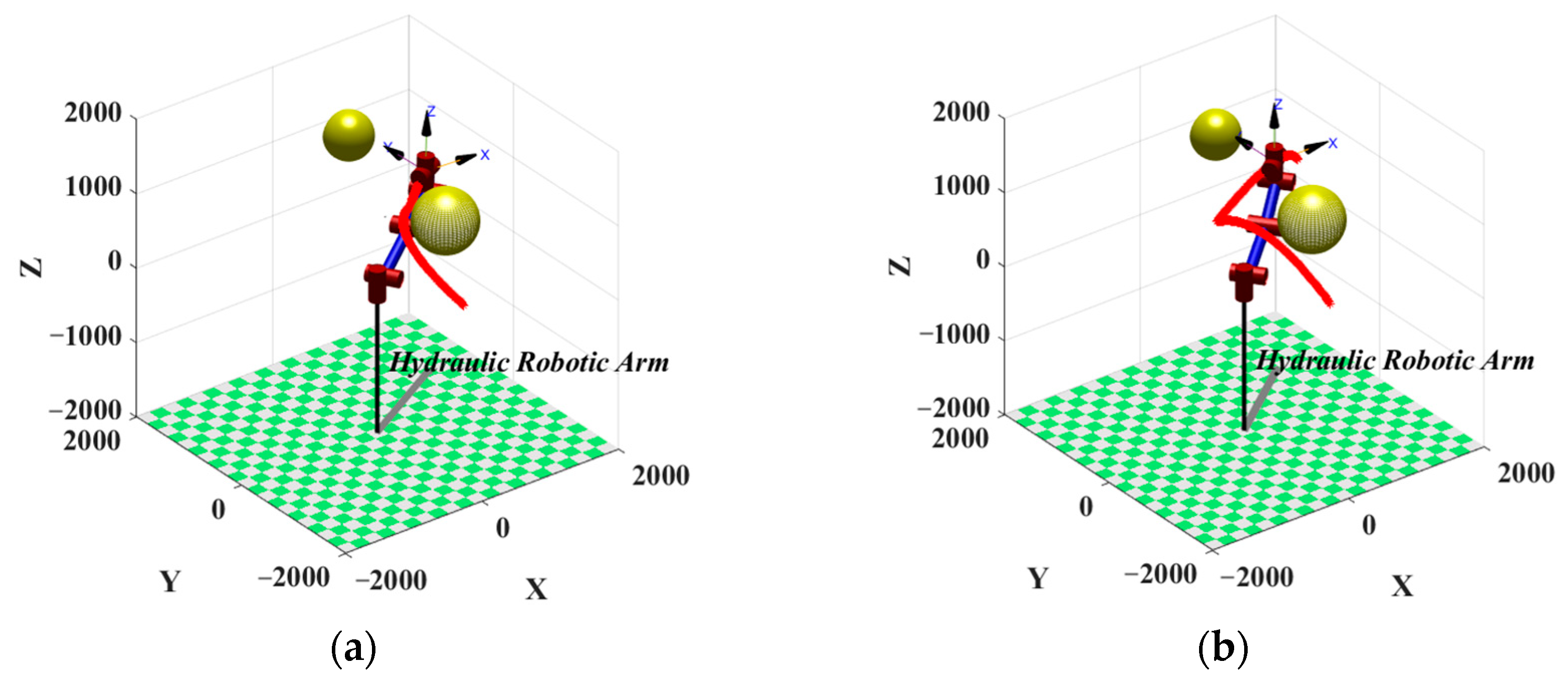
Through the robotics toolbox in MATLAB, the multi-strategy improved Gray Wolf Algorithm and basic Gray Wolf Algorithm were applied to a six-degree-of-freedom pile driving robotic arm, and the performance of the two algorithms was tested simultaneously in a 3D environment. The starting position of the path [500, −1000, 0] and the ending position [1800, 1800, 800] were set, and two obstacles were set in the environment, both of which were enveloped with spherical shapes. The simulation results are shown in

Table 4. Comparison results of two algorithms.

Algorithm	Path Length/mm	Average Path/mm	Running Time/s
Improved GWO	3751.04	3832.23	156.251
Basic GWO	4567.32	4593.62	172.561

and Figure 11, with the red line indicating the planned path. From Figure 11, it can be seen that both the improved GWO and the path planned by GWO can avoid obstacles and reach the target point, but the path planned by the improved GWO is shorter. From Table 4, it can be seen that compared to the basic GWO algorithm, the improved GWO algorithm reduces the 3D path length by 16.575% and the running time by 9.452%. In summary, it can be seen that compared to basic GWO algorithms, applying improved GWO algorithms to path planning on robotic arms yields better paths. Therefore, the improved algorithm can effectively achieve path planning and convert the expected displacement based on the given end effector’s expected pose coordinate value, in order to achieve the adjustment of the pile’s pose.

In the subsequent work, it is necessary to use sensors installed on the boom cylinder, stick cylinder, and four-bar drive cylinder to detect the real-time displacement of each group of cylinders in real time, and compare the detected real-time displacement of the cylinders with the expected displacement of the cylinders as input values for the controller. Once there is a deviation between the detected cylinder displacement and the expected cylinder displacement, GWO will play an adjusting role to eliminate the deviation between the two and achieve a real-time attitude adjustment of the pile towards the desired attitude. Thus, monitoring the pose of the end effector of the working device and adjusting the pose of the end effector of the working device are carried out for experimental verification.

5. Conclusions

Addressing the imperative need for adjusting the pile body posture in the context of the side-clamp vibrating pile driver, this study focused on the mechanical arm mechanism. The research outcomes are summarized as follows:

(1)

Taking the side-clamp vibration pile driver as the research object, an improved D-H parameter method was used to establish the kinematic model of the working device of the pile driver, and the kinematic equations were solved in forward and inverse kinematics. A mathematical model was established based on inverse kinematics to solve the joint angles and their corresponding hydraulic cylinder propulsion stroke. The forward and inverse kinematic models of the working device of the pile driver using the MATLAB robotics toolbox were simulated to verify the correctness of the kinematic models. And based on the Monte Carlo method, the motion space simulation of the working device was carried out to solve the working range of the mechanical arm of the pile driver.

(2)

A multi-strategy improved GWO path planning algorithm is proposed to address the issue of operators being unable to directly obtain the vertical posture of the pile due to limited field of view, making it difficult to operate. The improved Grey Wolf algorithm was successfully applied to the three-dimensional path planning problem of robotic arms. Compared with the basic GWO algorithm, the improved GWO algorithm reduced the three-dimensional path length by 16.575% and the running time by 9.452%. The expected rotation angle of each joint was efficiently converted into the expected displacement of its corresponding oil cylinder, in order to achieve real-time pose adjustment of the pile to the desired pose.

References

- Massarsch, K.R.; Fellenius, B.H. Engineering assessment of ground vibrations caused by impact pile driving. Geotech. Eng. J. SEAGS AGSSEA 2015, 46, 54–63. [Google Scholar]
- Holeyman, A.; Whenham, V. Critical Review of the Hypervib1 Model to Assess Pile Vibro-Drivability. Geotech. Geol. Eng. 2017, 35, 1933–1951. [Google Scholar] [CrossRef]
- Keskinen, E.; Launis, S.; Cotsaftis, M.; Raunisto, Y. Performance Analysis of Drive-Line Steering Methods in Excavator-Mounted Sheet-Piling Systems. Comput. Aided Civ. Infrastruct. Eng. 2001, 16, 229–238. [Google Scholar] [CrossRef]
- Sasaki, T.; Kawahara, H.; Inoue, F.; Hashimoto, H. Circle fitting based pile positioning and machine pose estimation from range data for pile driver navigation. IFAC Proc. Vol. 2012, 45, 848–853. [Google Scholar] [CrossRef]
- Huang, X.; Sasaki, T.; Hashimoto, H.; Inoue, F.; Zheng, B.; Masuda, T.; Ikeuchi, K. An accurate and efficient pile driver positioning system using laser range finder. In Advances in Depth Image Analysis and Applications: International Workshop, WDIA 2012, Tsukuba, Japan, November 11, 2012, Revised Selected and Invited Papers; Springer: Berlin/Heidelberg, Germany, 2013; pp. 158–167. [Google Scholar]
- Xie, Y.; Wang, Q.; Yao, L.; Meng, X.; Yang, Y. Integrated multi-sensor real time pile positioning model and its application for sea piling. Remote Sens. 2020, 12, 3227. [Google Scholar] [CrossRef]
- Inoue, F.; Sasaki, T.; Huang, X.; Hashimoto, H. Development of position measurement system for construction pile using laser range finder. In Proceedings of the 28th International Symposium on Automation and Robotics in Construction, Seoul, Republic of Korea, 29 June–2 July 2011; pp. 794–800. [Google Scholar]
- Sharma, S.; Ahmed, S.; Naseem, M.; Alnumay, W.S.; Singh, S.; Cho, G.H. A survey on applications of artificial intelligence for pre-parametric project cost and soil shear-strength estimation in construction and geotechnical engineering. Sensors 2021, 21, 463. [Google Scholar] [CrossRef] [PubMed]
- Han, G.; Seo, D.; Ryu, J.H.; Kwon, T.H. RootBot: Root-inspired soft-growing robot for high-curvature directional excavation. Acta Geotech. 2023, 1–13. [Google Scholar] [CrossRef]
- Berner, M.; Sifferlinger, N.A. Analysis of excavation methods for a small-scale mining robot. In ISARC. Proceedings of the International Symposium on Automation and Robotics in Construction; IAARC Publications: Kitakyushu, Japan, 2020; Volume 37, pp. 481–490. [Google Scholar]
- Isaka, K.; Tsumura, K.; Watanabe, T.; Toyama, W.; Sugesawa, M.; Yamada, Y.; Yoshida, H.; Nakamura, T. Development of underwater drilling robot based on earthworm locomotion. IEEE Access 2019, 7, 103127–103141. [Google Scholar] [CrossRef]
- Guan, D.; Yang, N.; Lai, J.; Siu, M.F.F.; Jing, X.; Lau, C.K. Kinematic modeling and constraint analysis for robotic excavator operations in piling construction. Autom. Constr. 2021, 126, 103666. [Google Scholar] [CrossRef]
- Sun, J.D.; Cao, G.Z.; Li, W.B.; Liang, Y.X.; Huang, S.D. Analytical inverse kinematic solution using the DH method for a 6-DOF robot. In Proceedings of the 2017 14th International Conference on Ubiquitous Robots and Ambient Intelligence (URAI), Jeju, Republic of Korea, 28 June–1 July 2017; pp. 714–716. [Google Scholar]
- Shrey, S.; Patil, S.; Pawar, N.; Lokhande, C.; Dandage, A.; Ghorpade, R.R. Forward kinematic analysis of 5-DOF LYNX6 robotic arm used in robot-assisted surgery. Mater. Today Proc. 2023, 72, 858–863. [Google Scholar] [CrossRef]
- Ge, W.; Li, L.; Xing, E.; Lei, M.; Yang, S.; Zielinska, T. Design Study of 6-DOF Grinding Robot. In Proceedings of the 2019 IEEE International Conference on Mechatronics and Automation (ICMA), Tianjin, China, 4–7 August 2019; pp. 285–290. [Google Scholar]
- Dou, R.; Yu, S.; Li, W.; Chen, P.; Xia, P.; Zhai, F.; Yokoi, H.; Jiang, Y. Inverse kinematics for a 7-DOF humanoid robotic arm with joint limit and end pose coupling. Mech. Mach. Theory 2022, 169, 104637. [Google Scholar] [CrossRef]
- Chen, P.; Liu, L.; Yu, F.; Li, H.; Yang, F.; Wang, X. A geometrical method for inverse kinematics of a kind of humanoid manipulator. Robot 2012, 34, 211–216. [Google Scholar] [CrossRef]
- Karakaya, S.; Kucukyildiz, G.; Ocak, H. A new mobile robot toolbox for MATLAB. J. Intell. Robot. Syst. 2017, 87, 125–140. [Google Scholar] [CrossRef]
- Luo, J.; Wen, Q.; He, J.; Ye, B. Workspace Analysis of 7-DOF Humanoid Robotic Arm Based on Monte Carlo Method. In Proceedings of the 2015 International Conference on Intelligent Systems Research and Mechatronics Engineering, Zhengzhou, China, 11–13 April 2015; pp. 48–51. [Google Scholar]
- Peidró, A.; Reinoso, Ó.; Gil, A.; Marín, J.M.; Payá, L. An improved Monte Carlo method based on Gaussian growth to calculate the workspace of robots. Eng. Appl. Artif. Intell. 2017, 64, 197–207. [Google Scholar] [CrossRef]
- Wang, C.; Han, Q.S. Kinematics of Six-degree-of-freedom Series Manipulator and Its Working Space. Modul. Mach. Tool Autom. Manuf. Tech. 2020, 6, 32–36. [Google Scholar]
- Han, T.; Li, J.; Huang, Y.; Xu, S.; Xu, J. Research on trajectory planning algorithm of manipulator arm of coal raine rescue robot. Ind. Mine Autom 2021, 47, 45–52. [Google Scholar]
- Szczepanski, R.; Bereit, A.; Tarczewski, T. Efficient local path planning algorithm using artificial potential field supported by augmented reality. Energies 2021, 14, 6642. [Google Scholar] [CrossRef]
- Szczepanski, R.; Tarczewski, T.; Erwinski, K. Energy efficient local path planning algorithm based on predictive artificial potential field. IEEE Access 2022, 10, 39729–39742. [Google Scholar] [CrossRef]
- Li, C.; Meng, F.; Ma, H.; Wang, J.; Meng, M.Q.H. Relevant region sampling strategy with adaptive heuristic for asymptotically optimal path planning. Biomim. Intell. Robot. 2023, 3, 100113. [Google Scholar] [CrossRef]
- Lei, T.; Chintam, P.; Carruth, D.W.; Jan, G.E.; Luo, C. Human-autonomy teaming-based robot informative path planning and mapping algorithms with tree search mechanism. In Proceedings of the 2022 IEEE 3rd International Conference on Human-Machine Systems (ICHMS), Orlando, FL, USA, 17–19 November 2022; pp. 1–6. [Google Scholar]
- Lei, T.; Chintam, P.; Luo, C.; Rahimi, S. Multi-Robot Directed Coverage Path Planning in Row-based Environments. In Proceedings of the 2022 IEEE Fifth International Conference on Artificial Intelligence and Knowledge Engineering (AIKE), Laguna Hills, CA, USA, 19–21 September 2022; pp. 114–121. [Google Scholar]
- Li, X.; Gao, X.; Zhang, W.; Hao, L. Smooth and collision-free trajectory generation in cluttered environments using cubic B-spline form. Mech. Mach. Theory 2022, 169, 104606. [Google Scholar] [CrossRef]
- Short, D.; Lei, T.; Luo, C.; Carruth, D.W.; Bi, Z. A bio-inspired algorithm in image-based path planning and localization using visual features and maps. Intell. Robot. 2023, 3, 222–241. [Google Scholar] [CrossRef]
- Wang, J.; Chen, W.; Xiao, X.; Xu, Y.; Li, C.; Jia, X.; Meng, M.Q.H. A survey of the development of biomimetic intelligence and robotics. Biomim. Intell. Robot. 2021, 1, 100001. [Google Scholar] [CrossRef]
- Rezoug, A.; Iqbal, J.; Tadjine, M. Extended grey wolf optimization–based adaptive fast nonsingular terminal sliding mode control of a robotic manipulator. Proc. Inst. Mech. Eng. Part I J. Syst. Control Eng. 2022, 236, 1738–1754. [Google Scholar] [CrossRef]
- Pehlivanoglu, Y.V.; Pehlivanoglu, P. An enhanced genetic algorithm for path planning of autonomous UAV in target coverage problems. Appl. Soft Comput. 2021, 112, 107796. [Google Scholar] [CrossRef]
- Shi, J.; Tan, L.; Zhang, H.; Lian, X.; Xu, T. Adaptive multi-UAV path planning method based on improved gray wolf algorithm. Comput. Electr. Eng. 2022, 104, 108377. [Google Scholar]
- Cheng, X.; Li, J.; Zheng, C.; Zhang, J.; Zhao, M. An improved PSO-GWO algorithm with chaos and adaptive inertial weight for robot path planning. Front. Neurorobotics 2021, 15, 770361. [Google Scholar] [CrossRef] [PubMed]
- Zhang, C.; Liu, Y.; Hu, C. Path planning with time windows for multiple UAVs based on gray wolf algorithm. Biomimetics 2022, 7, 225. [Google Scholar] [CrossRef]
- Qazani, M.R.C.; Asadi, H.; Arogbonlo, A.; Rahimzadeh, G.; Mohamed, S.; Pedrammehr, S.; Lim, C.P.; Nahavandi, S. Whale optimization algorithm for weight tuning of a model predictive control-based motion cueing algorithm. In Proceedings of the 2021 IEEE International Conference on Systems, Man, and Cybernetics (SMC), Melbourne, Australia, 17–20 October 2021; pp. 1042–1048. [Google Scholar]
- Deckner, F.; Viking, K. Wave patterns in the ground: Case studies related to vibratory sheet pile driving. Geotech. Geol. Eng. 2017, 35, 2863–2878. [Google Scholar] [CrossRef]
- Khan, M.F.; ul Islam, R.; Iqbal, J. Control strategies for robotic manipulators. In Proceedings of the 2012 International Conference of Robotics and Artificial Intelligence, Rawalpindi, Pakistan, 22–23 October 2012; pp. 26–33. [Google Scholar]
- Fausto, F.; Reyna-Orta, A.; Cuevas, E.; Andrade, Á.G.; Perez-Cisneros, M. From ants to whales: Metaheuristics for all tastes. Artif. Intell. Rev. 2020, 53, 753–810. [Google Scholar] [CrossRef]
- Bansal, J.C.; Singh, P.K.; Pal, N.R. (Eds.) Evolutionary and Swarm Intelligence Algorithms; Springer: Cham, Switzerland, 2019. [Google Scholar]
- Mirjalili, S.; Mirjalili, S.M.; Lewis, A. Grey wolf optimizer. Adv. Eng. Softw. 2014, 69, 46–61. [Google Scholar] [CrossRef]
Figure 1.
Working conditions of the vibratory pile driver.
Figure 2.
Swinging mechanism.
Figure 3.
Coordinate system of each joint of the robotic arm.